Dust Extinction in Compact Planetary Nebulae

Abstract

The effects of dust extinction on the departure from axi-symmetry in the morphology of planetary nebulae (PNs) are investigated through a comparison of the radio free-free emission and hydrogen recombination line images. The dust exctinction maps of five compact PNs are derived using high-resolution ($\sim$0$\farcs$1) H$\alpha$ and radio images maps of the HST and VLA. These extinction maps are then analyzed by an ellipsoidal shell ionization model including the effects of dust extinction to infer the nebulae’s intrinsic structure and orientation in the sky. This method provides a quantitative analysis of the morphological structure of PNs and represents a step beyond qualitative classification of morphological types of PNs.

1 Introduction

In general, PNs have axisymmetric structures. The classification of PNs into three basic types, round, elliptical and bipolar (Balick, 1987), is based on their axisymmetric appearances. However, many PNs also possess non-axisymmetric structures. Soker & Hadar (2002) proposed a scheme to classify PNs according to their departure from axisymmetry. They considered six categories: (1) PNs where the central star is not at the center of the nebula; (2) PNs having one side brighter than the other; (3) PNs having unequal size or shape of the two sides; (4) PNs where the symmetry axis is bent, e.g., the two lobes in a bipolar PN are bent toward the same side; (5) PNs where the main departure from axisymmetry is in the outer regions, e.g., an outer arc; (6) PNs showing no large-scale departure from axisymmetry. They found that about 50% of the analyzed sample has large-scale departures from axisymmetry.

The problem of departure from axisymmetry in PNs is usually investigated through the examination of optical images. This poses a problem because dust also plays a role in making such asymmetry. For example, in the sample analyzed by Soker & Hadar (2002), more than half of the PNs they found to have departure from axisymmetry are the types with unequal intensity or size. This kind of asymmetric appearance can also be caused by dust extinction, even if the intrinsic brightness of the nebula is axisymmetric. It is very difficult to draw conclusions about the real shapes of PNs based only on their apparent optical forms. In order to remove the bias caused by dust extinction while investigating the shapes of PNs, it is necessary to understand the dust distribution in PNs.

Asymptotic Giant Branch (AGB) stars eject large amount of dust and gas in the form of stellar winds. These stellar grains is a major source of dust grains in the Galaxy (Gehrz, 1989). Although the details of dust formation are still poorly understood, the properties of circumstellar dust have been extensively studied in the infrared, e.g., by the Infrared Astronomy Satellite (IRAS) and Infrared Space Observatory (ISO) missions. Since PNs descend from AGB stars, the remnants of the AGB dust envelopes should still be present in PNs (Kwok, 1982). The presence of dust in PNs was first detected in NGC 7027 via its infrared emission (Gillett, Low & Stein, 1967). This infrared excess peaks around 30 $\mu$m and has a color temperature of $\sim$100 K. Although the existence of dust in PNs first came as a surprise, its widespread presence is now confirmed by IRAS observations (Pottasch et al., 1984; Zhang & Kwok, 1991).

While the presence of dust in PNs is well established by infrared spectroscopy, very little is known about its spatial distribution. Recent development in mid-infrared cameras has just begun to explore the dust distribution of PNs (see, e.g., Volk & Kwok, 2003; Su et al., 2004). However, a full mapping of the dust distribution of PNs has to wait until the development of large-format mid-infrared cameras with high resolution and high sensitivity. An alternate and underutilized method to derive the dust distribution is by comparing the hydrogen recombination line map of a PN with its corresponding radio free-free continuum map. The recombination line (e.g. H$\alpha$) and free-free continuum emission are independent tracers of the distribution of the ionized gas, and both of their fluxes are proportional to $n_{e}^{2}V$ under optically thin conditions, where $n_{e}$ is the electron density and V is the volume of the nebula. If dust is present, they will have no effect on the long wavelength radio emission, but the H$\alpha$ emission will be attenuated by dust. Therefore the dust distribution can be indirectly obtained by comparing the H$\alpha$ and radio maps, assuming the dust is associated with the ionized gas. This method has been applied to different objects by various authors (e.g., Vázquez et al., 1999; Eyres et al., 2001). In this paper, we have derived optical depth maps of five compact PNs obtained with the same technique. Compact PNs are selected for this study because their small angular sizes allow the assumption that any foreground interstellar extinction is homogeneous over the entire object, so that the different degrees of extinction over a PN are only related to its internal dust distribution.

2 Derivation of the optical depth distribution

In a fully ionized region, both the free-free emission and the recombination fluxes are proportional to $n_{e}^{2}V$, where $n_{e}$ is the electron density. The ratio of the free-free flux to the H$\beta$ recombination line fluxes under Case B (where recombination to the ground state is excluded) is given by the following equation (Pottasch, 1984):

$$\frac{S_{\nu}({\rm ff})}{F({\rm H}\beta)}=2.51\times 10^{7}T_{e}^{0.53}\nu^{-0.1}Y~{}~{}~{}\rm\frac{Jansky}{erg~{}cm^{-2}s^{-1}}~{},$$ (1)

where $T_{e}$ is the electron temperature, and

$$Y=1+\frac{n(He^{+})}{n_{p}}+3.7\frac{n(He^{++})}{n_{p}}$$ (2)

corrects for the contribution to the free-free flux from He ions. For a He to H number ratio of 0.11 and for He to be equally divided between singly and doubly ionized forms, $Y$ has a value of 1.258. Under Case B, the effective recombination coefficients for H$\alpha$ and H$\beta$ have a ratio of 2.85 (Hummer & Storey, 1987). For $T_{e}=10^{4}$ K, eq. 1 can be written as

$$F_{{\rm exp}}({\rm H}\alpha)=6.85\times 10^{-10}(\nu/{\rm GHz})^{0.1}(S_{\nu}/{\rm Jy})~{}~{}~{}\rm erg~{}cm^{-2}~{}s^{-1}~{},$$ (3)

which can be used to calculate the expected flux of H$\alpha$ emission without dust extinction from the flux density of radio continuum emission.

In order to derive the extinction map, we begin with the radio continuum and H$\alpha$ maps of the same PN at similar angular resolutions. The expected H$\alpha$ emission at each pixel is derived from the radio continuum map, and then divided by the observed H$\alpha$ emission map for each object to obtain an extinction map, in which the dust optical depth at each pixel can be calculated. The intensity emitted by an object and received by the observer is related by the optical depth $\tau$ as

$$F_{\rm obs}=F_{\rm exp}e^{-\tau}~{},$$ (4)

where $F_{\rm exp}$ is the intensity emitted by the object, i.e., the intensity expected to be received by the observer if no dust is present. Therefore the dust optical depth for H$\alpha$ emission is obtained by taking the natural logarithm of the ratio of the expected and observed H$\alpha$ flux:

$$\tau_{{\rm H}\alpha}=\ln\frac{F_{exp}({\rm H}\alpha)}{F_{obs}({\rm H}\alpha)}~{}.$$ (5)

3 Sample selection and data processing

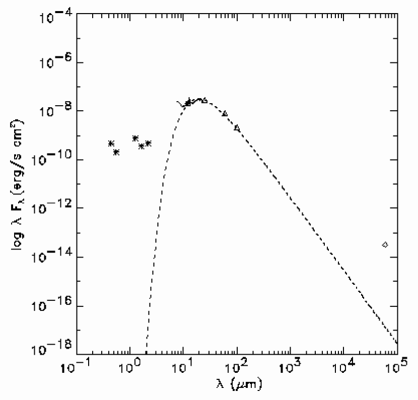
Figure 1: The SED of BD+30^∘3639, IC 5117, M 1-61, M 2-43, and M 3-45. The asterisk are ground-based optical and 2MASS measurements, the triangles are IRAS measurements, the crosses are MSX measurements, diamond are radio measurements, and the solid line is the IRAS LRS spectrum. The dashed line is the fitted blackbody curve for dust emission. The dust temperatures are BD+30^∘3639: $T_{d}=190\rm K$, IC 5117: 180 K, M 1-61: 170 K, M 2-43: 200 K, and M 3-35: 180 K.

In this paper, we have selected five compact PNs with known high infrared excesses. Figures 1 show the spectral energy distributions (SEDs) of these five PNs from optical to radio wavelengths, illustrating the IR excess caused by dust. The ground-based optical data are from Acker et al. (1992) and Acker, Marcout & Ochsenbein (1981). The near-infrared J, H, and K-band photometry are from the Two Micron All Sky Survey (2MASS), extracted from the 2MASS All-Sky Catalog of Point Sources (Cutri et al., 2003). The mid-infrared photometry includes IRAS photometry, IRAS low resolution spectra (LRS), and recent measurements from the Midcourse Space Experiment (MSX). The MSX measurements were extracted from the MSX Point Source Catalog (Egan et al., 2003). Radio photometric measurements (mostly at $\lambda$ 2 and 6 cm) are from Aaquist & Kwok (1990), Basart & Daub (1987), and this study. As clearly shown in Fig. 1, the infrared excess of the PNs is well represented by a single blackbody curve with a temperature $\sim$ 200 K.

High resolution H$\alpha$ and radio images of these PNs are available from the HST and the VLA respectively. The basic information for the five objects is listed in Table 1. With these high resolution images, the point-to-point spatial extinction distribution in PNs can be obtained with angular resolutions as high as $\sim$ 0.1 arcsec.

For IC 5117, M 1-61, M 2-43, and M 3-35, the HST WFPC2 H$\alpha$ images were obtained under the GO program 8307 (Kwok, Su & Sahai, 2003). For BD+30^∘3639, the HST WFPC2 H$\alpha$ image was first presented in Harrington et al. (1997) and the calibrated images were obtained from the HST archive. The only image processing needed was to remove cosmic rays with the task CRREJ in IRAF. The angular resolution FWHM of these images ranges from 0$\farcs$085 to 0$\farcs$11.

For BD+30^∘3639, the $\lambda$6 cm radio image was from Bryce et al. (1997). It was obtained by combining VLA and Multi-Element Radio Linked Interferometer Network (MERLIN) observations, resulting in a very high angular resolution of $\sim$ 0$\farcs$08. For the remaining four objects, the radio continuum maps were observed by Aaquist & Kwok with the VLA at $\lambda$2 cm in A-configuration in March 1998. The unpublished data were retrieved from the VLA archive and reduced using the package AIPS following the standard procedures of continuum data reduction, as summarized in Appendix A of the AIPS Cookbook (NRAO, 2003). After the data were calibrated, the final CLEAN images were generated with robust weighting in order to obtain images with minimum-noise levels while maintaining the highest angular resolution. This ranges from $\sim 0\farcs 12$ to $\sim 0\farcs 15$ in the final CLEAN maps.

The operations taken to combine the radio and optical data and to derive the optical depth map are performed in the following sequence. The HST images were first oriented north-up with Karma software. Subsequent regridding and other steps were performed in AIPS. Because the coordinates of the HST images have a uncertainty of $\sim 0\farcs 5$, there is usually an offset in the positions of the same object in the radio and optical images. To correct this, the H$\alpha$ images were shifted and aligned by eye to match with the radio continuum maps using features common in both images. Table 3 gives the offset of the coordinates for each object; a positive sign indicates the optical image has been shifted eastward or northward. Each object’s H$\alpha$ image was convolved with an extended Gaussian to match the beam size of the corresponding radio image, except for BD+30^∘3639. Because the radio continuum image of BD+30^∘3639 has a higher resolution than its H$\alpha$ image, it was convolved with an extended Gaussian to match the FWHM of the H$\alpha$ image. The radio image was transformed so that its pixel coordinate grid was consistent with that of the HST image. Division and natural logarithm operations were then performed to obtain an optical depth map as in eq. 5.

4 Results and Analysis

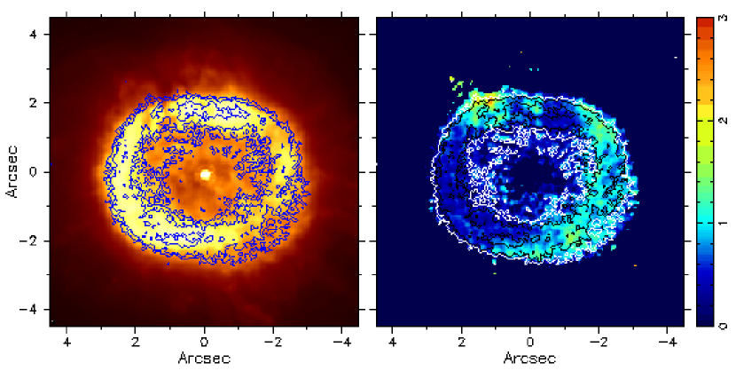
Figure 2: Images (from top to bottom) of BD+30^∘3639, IC 5117, M 1-61, M 2-43, M 3-35. Left panel: $\lambda$6 cm radio continuum (contours) on HST H$\alpha$ image (color, in square-root intensity scale). Right panel: $\lambda$6 cm radio continuum (contours) on extinction map (color). The color bar indicates $\tau$ values. BD+30^∘3639: The contour levels are $\sigma\times$ (3, 5, 10, 15) with the noise level $\sigma=4.5\times 10^{-5}$ Jy/beam. IC 5117: the contour levels are $\sigma\times$ (3, 5, 10, 15, 20, 25, 30, 40, 50) with the noise level $\sigma=8.89\times 10^{-5}$ Jy/beam. M 1-61: the contour levels are $\sigma\times$ (3, 5, 10, 15, 20, 25, 30, 35, 40, 45) with the noise level $\sigma=8.2\times 10^{-5}$ Jy/beam. M 2-43: the contours levels are $\sigma\times$ (3, 5, 10, 20, 30, 40, 50, 60, 70, 80) with the noise level $\sigma=1.11\times 10^{-4}$ Jy/beam. M 3-35: the color bar indicates $\tau$ values. The contour levels are $\sigma\times$ (3, 5, 10, 15, 20, 25, 30, 40, 50) with the noise level $\sigma=7.58\times 10^{-5}$ Jy/beam.

Extinction maps showing the dust optical depth for the five compact PNs are presented in Fig. 2. For comparison, the H$\alpha$ brightness and extinction maps for each object are shown side by side, and the corresponding radio continuum contours are superposed on both maps. All images are oriented with north up and east to the left.

4.1 BD+30^∘3639

The radio continuum image of BD+30^∘3639 shows a ring-like structure with two peaks of roughly the same brightness in the north and south regions. The H$\alpha$ image also shows a ring-like structure with two peaks. However, the ring shows unequal brightness in the east and west regions, which indicates the ring suffers more dust extinction in the west as shown in the optical depth map. The two high-extinction regions in the northeast and southwest are in roughly the same positions as the pair of high-velocity molecular knots found with CO line imaging by Bachiller et al. (2000).

4.2 IC 5117

The radio continuum image of IC 5117 shows a shell structure with two emission peaks. Such a shape can be simply explained as a prolate ellipsoidal shell projected onto the plane of the sky (Aaquist & Kwok, 1991). The H$\alpha$ image shows a similar structure with two pairs of faint bipolar lobes oriented at different angles (see image displayed by Kwok, Su & Sahai, 2003). The lobes are not seen in the radio continuum because of relatively low sensitivity for the radio map. The extinction map shows a similar structure to that of the radio map, where the high-extinction region follows the region of high brightness in radio. However, the two extinction peaks fall slightly outside of the radio peaks. A similar situation has been found in the dust extinction map of NGC 7027 (Walton et al., 1988).

4.3 M 1-61

The radio continuum image shows a shell structure with two pronounced emission peaks of roughly the same brightness. In the H$\alpha$ image, the eastern peak is weaker than the western peak, and there is at least one pair of faint bipolar lobes in the outer region (see image displayed by Kwok, Su & Sahai, 2003). The extinction map shows the optical depth is higher in the region of brighter radio emission, with a strong extinction peak near the eastern radio peak.

4.4 M 2-43

The radio continuum image shows a shell structure, with the southern peak brighter than the northern one. The H$\alpha$ image shows similar structure with slightly extended faint emission outside the radio emission region. However, the northern peak of H$\alpha$ emission is brighter than the southern one. As a result, although the structure of the extinction map mainly follows that of the radio map, the optical depth in the southern part is significant higher than the northern part. The extinction peaks also falls slightly outside of the radio peaks.

4.5 M 3-35

The radio continuum image shows a deep central emission minimum and two surrounding peaks with concave-like contours at roughly the same brightness. The H$\alpha$ image shows two peaks at approximately the same location with two pairs of faint bipolar lobes outside (see image displayed by Kwok, Su & Sahai, 2003). The extinction map has similar structure to that of the radio map, with the high-extinction region coinciding with the concave-like region.

4.6 Uncertainties in the Optical Depth

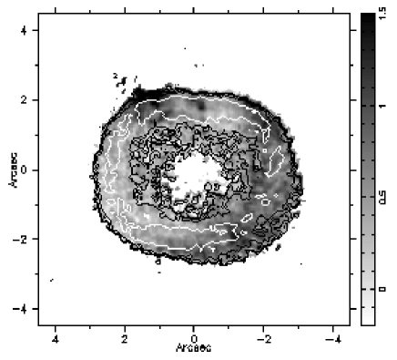
Figure 3: Uncertainty optical depth (contours) of (from top to bottom): BD+30^∘3639, IC 5117, M 1-61, M 2-43, M 3-35. superposed on the optical depth map in greyscale. The contours levels are BD+30^∘3639: 0.1, 0.2, 0.3, and 0.4, with 0.1 showing in white. IC 5117: 0.02, 0.04, 0.06, 0.08, 0.1, and 0.2, with 0.02 showing in white. M 1-61: 0.03, 0.06, 0.09, 0.12, 0.2, and 0.3, with 0.03 showing in white. M 2-43: 0.02, 0.05, 0.1, 0.2, and 0.3, with 0.02 showing in white. M 3-35: 0.03, 0.06, 0.09, 0.12, and 0.2, with 0.03 showing in white.

Figure 3 show the uncertainties propagated from the radio and optical images. The uncertainty associated with the optical depth $\tau$ is given by

$$\Delta\tau=\sqrt{\left(\frac{\sigma_{\rm radio}}{F_{\rm radio}}\right)^{2}+\left(\frac{\sigma_{\rm H\alpha}}{F_{\rm H\alpha}}\right)^{2}}$$ (6)

where $\sigma_{\rm radio}$ and $\sigma_{\rm H\alpha}$ are the rms noise of the radio continuum and optical H$\alpha$ images, respectively. Since the optical images have higher signal-to-noise ratios, the uncertainty of the optical depth is dominated by the radio image. Hence the uncertainty map of the optical depth and the radio continuum map have similar structure. The optical depth uncertainty ranges from $\Delta\tau\sim$ 0.01 to 0.4, where smaller values lie in the regions with stronger radio emission.

The calculations of optical depth above use several assumptions. To investigate whether the optical depth is sensitive to these assumptions, the uncertainties propagated from them should also be examined. Among these approximations, the electron temperature $T_{e}$ gives the most significant uncertainty. While most PNs have $T_{e}$ in the vicinity of 10,000 K, the electron temperatures of PNs cover a range of 5,000 - 15,000 K, with $T_{e}\sim$ 20,000 K in some extreme cases. As a result, different choices of $T_{e}$ will give different values of optical depth.

To calculate the uncertainty propagated from the assumption that $T_{e}=10,000$ K, we estimate the uncertainty for $T_{e}$ to be roughly $\Delta T_{e}=\pm 5,000$ K. Since $\tau\propto\ln F_{\rm exp}({\rm H}\alpha)\propto\ln T_{e}^{-0.53}$, the uncertainty propagated into the optical depth is $\Delta\tau\propto 0.53\times\frac{\Delta T_{e}}{T_{e}}\propto 0.53\times\frac{5,000}{10,000}\sim 0.27$. This value is an order of magnitude smaller than the derived optical depth. This uncertainty from the electron temperature will only shift the values of the derived optical depths by a constant, but will not change the overall appearance of the extinction caused by its dust in a PN.

4.7 Dust distribution

All five PNs in this study show that the H$\alpha$ emission peaks and the radio continuum emission peaks are in the same regions. In four of them, the peaks of the dust extinction also reside in the same regions. These results suggest that the ionized gas and the dust have similar distributions, so at least part of the dust is mixed with the ionized gas.

On the quantative scale, the faintest parts of the optical image correlate with the peaks of the extinction distribution, as is expected. As an independent check, Kastner et al. (2002) compared the X-ray emission map of BD+30^∘3639 with its extinction map derived from optical and infrared images, and showed that the peak of X-ray emission also lies in the region with minimum extinction.

We note that the radio images, H$\alpha$ images, and the dust optical depth maps only represent the column density distribution along the line of sight. In order to remove projection effects and reconstruct the three dimensional ionized gas and dust distributions in PNs, we need to develop a 3-D model. The details of the model analysis are presented in the next section.

5 The Three Dimensional Dusty Ellipsoidal Shell (DES) Model

While the classification of PN morphology is based on appearance, this approach is vulnerable to projection effects. For example, elliptical and bipolar nebulae can appear round when the nebulae are viewed pole-on. In order to study their intrinsic properties, there have been many attempts to find the detailed three-dimensional structures of PNs (Khromov & Kohoutek, 1968). Since many PNs have the appearance of limb-brightened elliptical rings that are brightest on their minor axes, it is natural to consider models in which the nebulae have an elongated, hollow shell structure. Models with this simple geometry, such as the prolate ellipsoidal shell discussed by Masson (1989, 1990), are successful in reproducing many of the shapes observed in PNs. This was followed by the work of Aaquist & Kwok (1996) who developed a prolate ellipsoidal shell (PES) model to fit the radio images of PNs. Their model contains a spherical shell with both radial and latitude-dependent density gradients, and the shell is ionized by a central star to various depths at different latitudual directions. The ionized shell, when viewed at different angles, results in a variety of morphologies seen in PNs. The parameters derived from the PES model reveal the asymmetric distribution of the ionized gas in the nebula. The PES model was later called the ES model and explored extensively by Zhang & Kwok (1998) to investigate the statistical distributions of the asymmetry parameters. However, because of a typographical error in the source code, there are some uncertainties in the derived model parameters in Zhang & Kwok (1998).

In order to simulate dust extinction effects, we have modified the ES model to include a dust distribution with a constant gas-to-dust ratio, and we refer to this model as the dusty ellipsoidal shell (DES) model. The DES model has been used to analyze the observational images, including radio continuum, H$\alpha$, and dust extinction maps to constrain the ionized gas and dust distributions in compact PNs. These different images of the same object provide a way to study the distribution of dust in PNs, and also give better constraints on the model parameters than a single radio or optical image would. One advantage of using the model is that it helps to remove projection effects and to construct the three-dimensional structures of PNs. The DES model will give a quantitative classification of PNs morphology rather than the standard descriptive terms such as round, elliptical, or bipolar.

5.1 The Geometry of the DES model

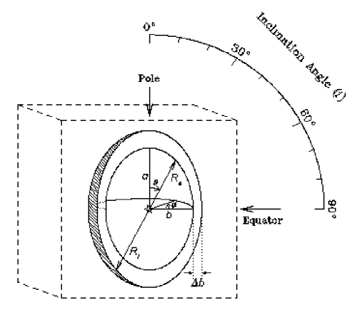
Figure 4: Geometry of the dusty ellipsoidal shell model. The inclination angle i, measured in the ab plane, marks the direction toward the observer.

The geometry of the DES model is shown in Figure 4. A single (hot) star is located inside a shell of ionized gas. The inner region of the nebula is assumed to be empty, supposedly swept clean by a wind from the central star. For simplicity, the empty region is assumed to be a prolate or oblate spheroid, depending on the choice of polar radius a and equatorial radius b. The shape of the shell is the result of the interacting winds process, where either the slow AGB wind is equatorially enhanced, or the fast central star wind is non-isotropic (e.g. collimated), or both. The distance from the star to the inner edge of the gas $R_{s}$ can be calculated from a, b and the polar angle $\theta$. The UV photons from the central star ionize the surrounding gas out to the distance $R_{i}$, which depends upon $R_{s}$ and the density structure of the surrounding nebula.

The model assumes the central star is emitting ionizing photons isotropically, and the ionized nebula is ionization-bounded along any radial directions from the central star. The depth of the ionization front along any radial vector is given approximately by

$$\frac{dL}{d\Omega}=\alpha_{B}\int_{R_{s}}^{R_{i}}n^{2}(r,\theta,\phi)r^{2}dr~{},$$ (7)

where $dL/d\Omega$, the number of local ionizing photons ($L$) per unit solid angle ($\Omega$), is set equal to the total number of recombinations within the local ionized region. In this equation, $\alpha_{B}$ is the recombination coefficient excluding captures to the ground level (Case B approximation), $n(r,\theta,\phi)$ is the density structure of the swept-up shell, and $r,~{}\theta,~{}\phi$ are the spherical coordinates. $R_{i}$ is a function of $\theta$ and $\phi$ that depends on the density distribution. For simplicity, a separable density law is assumed, so that $n(r,\theta,\phi)=n_{0}\eta_{r}\eta_{\theta}\eta_{\phi}$; here $n_{0}$ is the density at the inner edge, where $(r,\theta,\phi)=(R_{s},0,0)$, and $\eta_{r},~{}\eta_{\theta},~{}\eta_{\phi}$ are dimensionless quantities describing the density relative to $n_{0}$:

$$\eta_{r} = (r/R_{s})^{-\gamma}$$ (8)

$$\eta_{\theta} = f_{\theta}\times\left\{\begin{array}[]{lr}(1-\beta)\displaystyle\left(\frac{2\theta}{\pi}\right)^{\alpha}+\beta,&\quad\mbox{if $0\leq\theta\leq\displaystyle\frac{\pi}{2}$}\\ \\ (1-\beta)\displaystyle\left(\frac{2\pi-2\theta}{\pi}\right)^{\alpha}+\beta,&\quad\mbox{if $\displaystyle\frac{\pi}{2}\leq\theta\leq\pi$}\end{array}\right\}$$ (12)

$$\eta_{\phi} = f_{\phi}~{}.$$ (13)

In this formulation, $\gamma$ gives the logarithmic radial density gradient, $\beta$ gives the pole-to equator density ratio, $\alpha$ governs the shape of the angular density function, and $f_{\theta},f_{\phi}$ are additional asymmetry factors:

$$f_{\theta} = \delta_{\theta}+(1-\delta_{\theta})exp[\cos(\theta-\theta_{0})-1];\ \ \ 0\leq\delta_{\theta}\leq 1$$ (14)

$$f_{\phi} = \delta_{\phi}+(1-\delta_{\phi})exp[\cos(\phi-\phi_{0})-1];\ \ \ 0\leq\delta_{\phi}\leq 1~{},$$ (15)

where these control asymmetry in the latitude ($\theta$) and longitude ($\phi$) directions, respectively. These two asymmetry factors are used to produce the departure from axisymmetry seen in many PNs. For simplicity, the phases $\theta_{0}$ and $\phi_{0}$ are both assumed to be $0^{\circ}$, so that $f_{\theta}$, $f_{\phi}$ are maximized (=1) for $\phi=0^{\circ}$ and $\phi=0^{\circ}$, and minimized for $\phi=180^{\circ}$ and $\phi=180^{\circ}$.

With the given radial density law $\eta_{r}$, eq. 7 can be integrated to give a simple analytical solution:

$$\frac{dL}{d\Omega} = \alpha_{B}\int_{R_{s}}^{R_{i}}(n_{0}\eta_{r}\eta_{\theta}\eta_{\phi})^{2}r^{2}dr$$ (16)

$$= (n_{0}\eta_{\theta}\eta_{\phi})^{2}\alpha_{B}\int_{R_{s}}^{R_{i}}r^{-2\gamma+2}R_{s}^{2\gamma}dr$$

$$= (n_{0}\eta_{\theta}\eta_{\phi})^{2}\alpha_{B}R_{s}^{3}\frac{(R_{i}/R_{s})^{-2\gamma+3}-1}{-2\gamma+3}~{}.$$

Once the parameters describing the inner boundary, the density law ($\gamma,\eta_{\theta},\eta_{\phi}$), and the equatorial axis shell thickness $\Delta b=[R_{i}-R_{s}]_{\theta=90^{\circ}}$ are chosen, the outer ionized boundary $R_{i}(\theta,\phi)$ can be calculated from eq. 16.

The ionized shell is then projected onto the plane of the sky at different inclination angles i. For $i=0^{\circ}$, the nebula is seen pole-on, i.e., the line of sight is perpendicular to the equatorial plane. The edge-on case has $i=90^{\circ}$, with the line of sight in the equatorial plane. The projected emission from the ionized region is calculated by assuming that the intensity of the recombination H$\alpha$ line and the radio continuum emission is proportional to the integration of the square of the density function along the line of sight (eqs. 8 – 15). The calculations were done inside a cubic box containing the nebula.

To simulate optical extinction effect, we assume that the dust is well mixed with the gas in the ionized region. Thus, a constant gas-to-dust ratio is assigned throughout the ionized region, i.e., the amount of extinction is directly proportional to the density function at each integration point. The H$\alpha$ emission is then attenuated by the dust extinction using eq. 4.

5.2 The Model Images

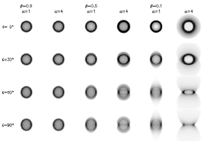
Figure 5: Model radio images assuming no radial density gradient ($\gamma=0$). The images from top to bottom show the effect of inclination for $i=0^{\circ},30^{\circ},60^{\circ}$ and $90^{\circ}$ with different combinations of $\beta$ and $\alpha$. The first pair of columns has $\beta=0.9$, with $\alpha=1$ and 4, respectively. The second and third pairs have $\beta=0.5$ and 0.1, also with $\alpha=1$ and 4. All images are on a linear grey scale.

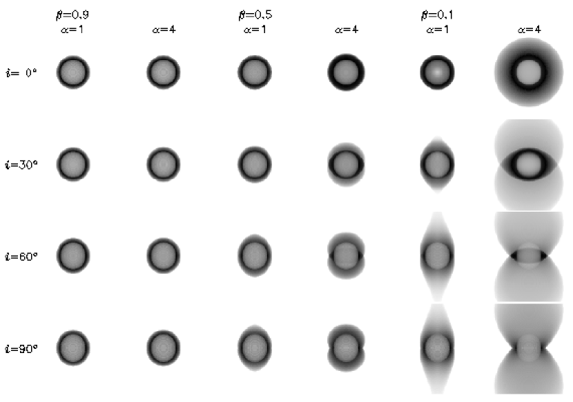
Figure 6: Input model dust distributions using the same parameters as in Figure 5. Each dust distribution simulates the dust extinction at optical wavelengths, although only the dust in front of the emitting gas will contribute to the optical extinction (see text for discussion).

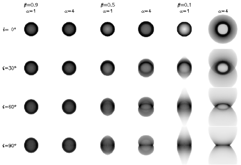
Figure 7: Model optical images with dust extinction included. The parameters are the same as in Figure 5.

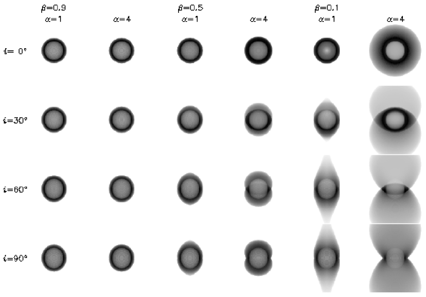
Figure 8: Derived extinction images. The optical depths are calculated by taking the natural logarithm of the ratio of the model radio and optical images. The images are arranged in the same order as in Figure 5.

The DES model allows us to explore how the morphology of a nebula changes with various parameters, especially $\alpha$ and $\beta$. A series of $128\times 128$ pixel model images has been produced with fixed parameters of $a=20,b=18$, and $\Delta b=6$. The model images presented here have no radial density gradient, i.e., $\gamma=0$. This is a fairly good approximation, because most swept-up shells are thought to be relatively thin, allowing little density change with radius. We have computed the projected images for inclination angles $i=0^{\circ},30^{\circ},60^{\circ}$, and $90^{\circ}$ with different combinations of $\beta$ and $\alpha$ as shown in Figures 5 – 8.

Figure 5 shows the model images with emission calculated from the integration of the square of the density function along the line of sight. This simulates the radio continuum images of the long-wavelength free-free emission not affected by dust.

Figure 6 displays the input dust distribution. The images are computed from the integration of the amount of extinction along the line of sight all the way through the nebula. Because the gas-to-dust ratio is constant inside the ionized region, the dust distributions appear similar to the model radio images in Figure 5. If the dust temperature is uniform, and the cloud is optically thin for the dust thermal emission, the flux emitted by the dust is directly proportional to the absorption coefficient. Therefore, these dust distributions can mimic infrared images of the dust emission.

Figure 7 gives the model images when the dust extinction is taken into account. As in Figure 5, emission is calculated from the integration of the square of the electron density, but now it is attenuated by the dust in front of it along the line of sight. This simulates the optical H$\alpha$ images, which, unlike the radio continuum maps, are affected by dust. Some images clearly show an asymmetric appearance caused by dust extinction (e.g., the image of $\alpha=1,~{}\beta=0.1,$ and $i=30^{\circ}$).

Figure 8 displays output extinction optical depth maps, calculated as the natural logarithm of the ratio of the model radio and optical images (eq. 5). Because only dust in front of the emission can attenuate the light, the amount of dust in the extinction maps (Fig. 8) is less than the actual amount of dust in the nebulae (Fig. 6). Comparing these images with the input dust distributions in Figure 6, the amount of missing dust for different inclination angles and morphologies can be estimated. By comparing the radio and H$\alpha$ images, the nebular geometry can be estimated and the asymmetry effect caused by dust for this viewing geometry can be removed and reveal any intrinsic asymmetry of the gas distribution.

6 Comparison of Observed and Model Images

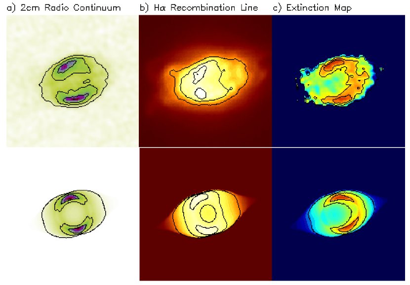
Figure 10: Comparison of the model with the observed images for IC 5117. The observed images are in the top panels and the model images are in the bottom panels. The images are: a) $\lambda$ 2 cm radio continuum emission. b) HST H$\alpha$ emission (Kwok, Su & Sahai, 2003). c) Extinction map derived from the radio continuum and H$\alpha$ emission. The radio and extinction images are displayed on a linear scale whereas the HST images are in square-root scale.

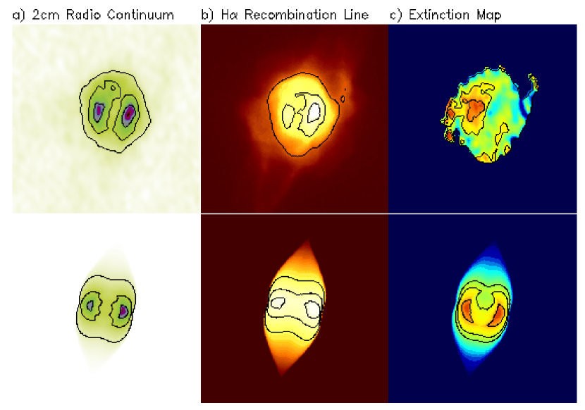
Figure 11: Comparison of the model with the observed images for M 1-61. The images are arranged in the same manner as Fig. 10.

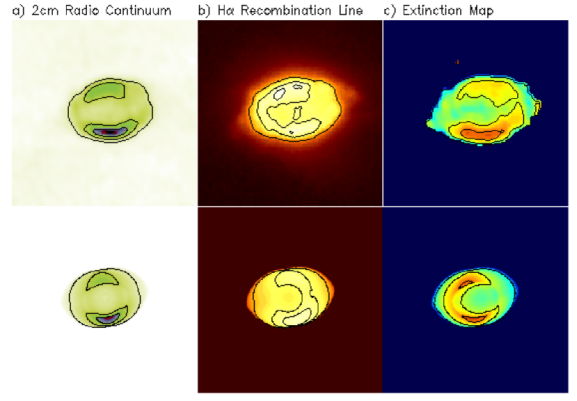
Figure 12: Comparison of the model with the observed images for M 2-43. The images are arranged in the same manner as Fig. 10.

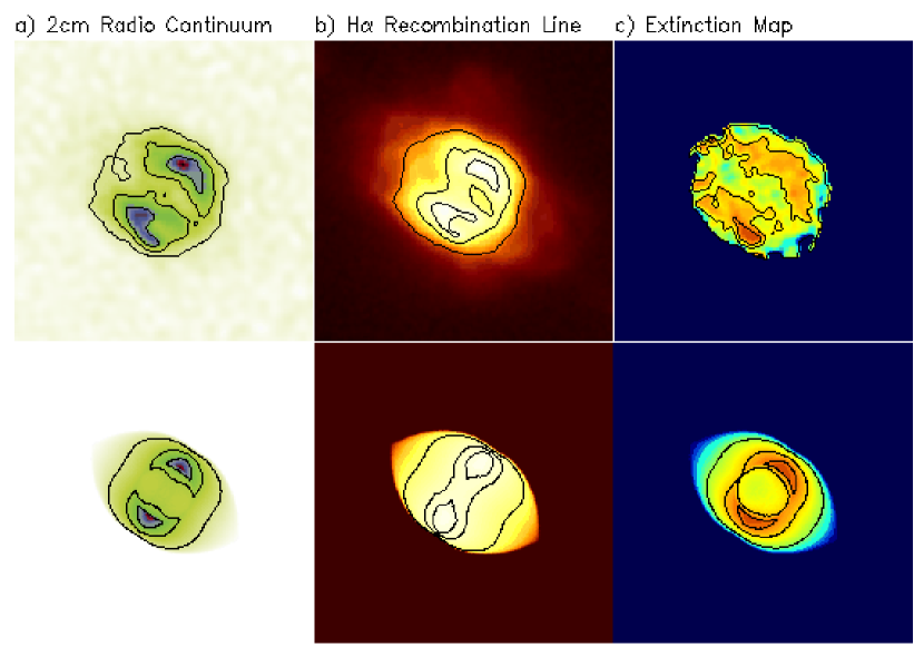
Figure 13: Comparison of the model with the observed images for M 3-35. The images are arranged in the same manner as Fig. 10.

In order to constrain the parameters that describe the geometry and angular density distribution of the PNs presented, a set of model images were made to compare to each individual nebula’s observed radio continuum and H$\alpha$ images, extinction maps, and in one case (BD+30^∘3639), an infrared dust emission image (from Volk & Kwok, 2003). The comparison was made by visual inspection. The faint emission from the outer parts of each nebula was chosen to match the observed H$\alpha$ images because their S/N ratios are much higher than those for the radio continuum images. For each object, a set of parameters was found that generate model images matching most of the observed images. The images comparing the best models to the observations for these five nebulae are shown in Figures 9 – 13. The parameters used to generate the model images are listed in Table 4.

6.1 BD+30^∘3639

The model of BD+30^∘3639 has a relatively small equatorial thickness $\Delta b$ compared to the size of the inner empty region, which has a prolate shape with an axial ratio of $a/b=1.2$. The small value of $\beta(=0.1$) suggests that it has a large equatorial to polar density ratio. A small asymmetry $\delta_{\phi}=0.9$ in the longitude direction is added to explain the unequal intensity of the two sides observed in the radio image. Dust well-mixed with ionized gas is able to reproduce the anti-correlation of the optical image and extinction map. Due to its low inclination angle ($i=15^{\circ}$), it has a round appearance. This low inclination is consistent with the value of $i\sim 10^{\circ}$ found by Li, Harrington & Borkowski (2002), who also fit the radio image and the spectra by approximating the nebula as an ellipsoid. But a comparison with the model image in Fig. 7 (second column from the right) suggests that BD+30^∘3639 would appear as a prominent bipolar nebula if viewed edge-on.

6.2 IC 5117

The model of IC 5117 also has a relatively small equatorial thickness compared to the inner empty region, with a prolate axial ratio $a/b=1.67$. It has a small pole-to-equator ratio of $\beta=0.1$. No asymmetry factor in the longitude direction is needed. The brighter region toward the east in the optical image and the higher extinction toward the west can be reproduced by a dust distribution with a constant gas-to-dust ratio. The model images have an intermediate inclination angle of $i=40^{\circ}$.

6.3 M 1-61

The model of M 1-61 has an equatorial thickness comparable to the dimension of the inner empty region, which has a prolate axial ratio of $a/b=1.2$. It has a small pole-to-equator ratio of $\beta=0.2$. A small asymmetry $\delta_{\phi}=0.9$ in the longitude direction is needed to explain the mildly brighter western peak in the radio image. The anti-correlation of the optical bright peak in the west and the strong extinction peak in the east can be reproduced by the well-mixed dust. However, it is not as prominent as the observed images. The model images has a high inclination angle of $i=70^{\circ}$, and they suggest that a higher dynamic range image of M 1-61 will reveal a pair of bipolar lobes.

6.4 M 2-43

The model of M 2-43 also has a relatively small equatorial thickness compared to the inner empty region with a prolate axial ratio $a/b=1.67$. It has a relatively small pole-to-equator ratio of $\beta=0.3$. A mild asymmetry $\delta_{\phi}=0.7$ in the longitude direction is added to reproduce the brighter southern peak in the radio image. Although a simple constant gas-to-dust ratio is able to generate an anti-correlation between the H$\alpha$ emission and optical depth, it cannot reproduce optical and extinction maps that match the observed images well. The model images have an intermediate inclination angle of $i=45^{\circ}$.

6.5 M 3-35

The model of M 3-35 has an equatorial thickness comparable to the dimension of the inner empty region, which has an oblate axial ratio of $a/b=0.83$. This is the only object that requires an oblate model. It has a intermediate pole-to-equator ratio of $\beta=0.4$. No asymmetry factor in the longitude direction is needed to reproduce the radio image. No obvious anti-correlation between optical and extinction maps can be found. The model images are highly inclined to the line of sight, with $i=80^{\circ}$. As in M 1-61, a higher dynamic range image is expected to reveal the bipolar lobes in the NE-SW directions.

7 Discussion

As we can see from Figures 9 – 13, the model images can generally simulate the observed images. The remaining differences could be accounted for by several effects. For example, the assumed model geometry may be too simple to reproduce all of the complex small-scale structure of PNs. Other causes could include clumpy dust distributions that do not follow a simple constant gas-to-dust ratio. Three out of five PNs show an asymmetric density distribution in the longitudinal direction, a departure from axisymmetry. As summarized by Soker & Rappaport (2001), four main processes can result in the departure from axisymmetry in PNs: interaction with the interstellar medium, mass-loss enhancements due to cool starspots, or a wide or a close binary companion. They investigated the effects of companions and estimated that about 27% of all PNs are expected to acquire non-axisymmetric structure from binary interactions. Nevertheless, the effects of the ISM are also worth considering. Since the majority of PNs are distributed near the Galactic plane where the mean density of the ISM is higher, significant interaction between PNs and the ISM is expected. Such phenomena can be seen from the disturbed emission on the outskirts of some nebulae (e.g., Xilouris et al., 1996) and from some apparently off-centered nuclei (e.g., Sh 2-216, Tweedy et al. 1995; KFR 1 and MeWe 1-4, Rauch et al. 2000).

The electron densities of these five PNs are all found to be higher near their equators than near their poles. The small pole-to-equator density ratios ($\beta$) of some nebulae indicate they would show a bipolar morphology if seen edge-on. The fraction of intrinsic bipolar PNs therefore are likely to be higher than suggested by classification by apparent morphology. Since the morphology of PNs has been proposed to relate to their physical properties, (e.g., bipolar nebulae have been suggested to correlate with nebulae with more massive central stars; Stanghellini, Corradi, & Schwarz, 1993), it is therefore important that we have a good understanding of the intrinsic strucures of PNs. By using models such as DES, we can more reliably estimate the fraction of bipolar nebulae and therefore assess any correlation with physical properties of the PNs.

8 Conclusions

We have derived the dust distribution in five compact PNs from their H$\alpha$ and radio images. From this study, we are able to determine the extent of contribution by dust extinction to the apparent departure from axi-symmetry in these PNs. By comparing these results with simulations generated by the ellipsoidal shell model, we can infer the intrinsic morphologies of the PNs. This method gives a more quantitative approach to the analysis of PN morphology than visual inspection of apparent morphology, and is therefore more capable to deducing proper statistics on the distribution of morphological types of PNs.

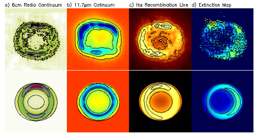
Figure 9: Comparison of the model with the observed images for BD+30^∘3639. The observed images are in the top panels and the model images are in the bottom panels. The images are: a) 6-cm radio continuum emission (Bryce et al., 1997). b) Gemini 11.7$\mu$m emission (Volk & Kwok, 2003). c) HST H$\alpha$ emission (from HST archive). d) Extinction map derived from the radio continuum and H$\alpha$ emission. All displays are on a linear scale except the HST observed and model images are in square-root of intensity.

Table 1: Basic Information for five compact PNs

Object	PN G	RA	Dec	Radio Diameter (′′)
BD+30∘3639	$064.7+05.0$	19:34:45.2	$+$30:30:59	6
IC 5117	$089.8-05.1$	21:32:31.0	$+$44:35:48	1.5
M 1-61	$019.4-05.3$	18:45:56.0	$-$14:27:42	1.8
M 2-42	$027.6+04.2$	18:26:40.2	$-$02:42:58	1.5
M 3-35	$071.6-02.3$	20:21:03.8	$+$32:29:22	1.5

Table 2: The angular resolutions of the radio and optical images

Object	VLA		HST
	Beam size (′′)	Beam PA (∘)	FWHM (′′)
BD+30∘3639	0.082 $\times$ 0.078	-28.37	0.11
IC 5117	0.13 $\times$ 0.12	-85.27	0.085
M 1-61	0.20 $\times$ 0.14	15.98	0.085
M2 43	0.15 $\times$ 0.13	25.51	0.095
M 3-35	0.12 $\times$ 0.12	-81.02	0.085

Table 3: The angular distances shifted in H$\alpha$ images

Object	Eastward (′′)	Northward (′′)	Offset Distance (′′)
BD+30∘3639	$-0.364$	$-0.455$	0.583
IC 5117	$-0.536$	$-0.378$	0.656
M 1-61	$-0.261$	$+0.261$	0.369
M 2-43	$+1.548$	$-0.273$	1.572
M 3-35	$-1.138$	$-0.299$	1.177

Table 4: DES model parameters of planetary nebulae

Object	$a$	$b$	$\Delta b$	$\beta$	$\alpha$	$i$	$\delta_{\phi}$	$\delta_{\theta}$
BD+30∘3639	18	15	5	0.1	1	15	0.9	1
IC5117	20	12	5	0.1	1	40	1	1
M1-61	12	10	8	0.2	1	70	0.9	1
M2-43	20	12	6	0.3	1	45	0.7	1
M3-35	10	12	10	0.4	1	80	1	1

References

- Aaquist & Kwok (1996) Aaquist, O. B., & Kwok, S. 1996, ApJ, 462, 813
- Aaquist & Kwok (1991) Aaquist, O. B., & Kwok, S. 1991, ApJ, 378, 599
- Aaquist & Kwok (1990) Aaquist, O. B., & Kwok, S. 1990, A&AS, 84, 229
- Acker, Marcout & Ochsenbein (1981) Acker, A., Marcout, J., & Ochsenbein, F. 1981, A&AS, 43, 265
- Acker et al. (1992) Acker, A. et al. 1992, Strasbourg-ESO Catalogue of Galactic Planetary Nebulae (Strasbourg: Obs. Strasbourg)
- Bachiller et al. (2000) Bachiller, R., Forveille, T., Huggins, P. J., Cox, P., & Maillard, J. P. 2000, A&A, 353, L5
- Balick (1987) Balick, B. 1987, AJ, 94, 671
- Basart & Daub (1987) Basart, J. P., & Daub, C. T. 1987, ApJ, 317, 412
- Bryce et al. (1997) Bryce, M., Pedlar, A., Muxlow, T., Thomasson, P., & Mellema, G. 1997, MNRAS, 284, 815
- Cutri et al. (2003) Cutri, R. M., et al. 2003, 2MASS All-Sky Catalog of Point Sources
- Egan et al. (2003) Egan M.P., Price S.D., Kraemer K.E., Mizuno D.R., Carey S.J., Wright C.O., Engelke C.W., Cohen M., & Gugliotti G. M. 2003, The Midcourse Space Experiment Point Source Catalog Version 2.3 (Air Force Research Laboratory Technical Report AFRL-VS-TR-2003-1589)
- Eyres et al. (2001) Eyres, S. P. S., Bode, M. F., Taylor, A. R., Crocker, M. M., & Davis, R. J. 2001, ApJ, 551, 512
- Gehrz (1989) Gehrz, R. D. 1989 in IAU Symp. 135, Interstellar Dust, eds. L. J. Allamandola, & A. G. G. M. Tielens (Kluwer: Dordrecht), p. 445
- Gillett, Low & Stein (1967) Gillett, F. C., Low, F. J., & Stein, W. A. 1967, ApJ, 149, L97
- Gooch (1996) Gooch, R. 1996, in ASP Conf. Ser. 101, Astronomical Data Analysis Software and Systems V, ed. G. H. Jacoby & J. Barnes (San Francisco: ASP), 80
- Harrington et al. (1997) Harrington, J. P., Lame, N. J., White, S. M., & Borkowski, K. J. 1997, AJ, 113, 2147
- Hummer & Storey (1987) Hummer, D. G., & Storey, P. J. 1987, MNRAS, 224, 801
- Kastner et al. (2002) Kastner, J. H., et al. 2002, ApJ, 2002, 581, 1225
- Khromov & Kohoutek (1968) Khromov, G.S., & Kohoutek, L. 1968, in IAU Symp. 34: Planetary Nebulae, eds. D.E. Osterbrock, & C.R. O’Dell (Reidel:Dordrecht), 227
- Kwok (1982) Kwok, S. 1982, ApJ, 258, 280
- Kwok, Su & Sahai (2003) Kwok, S., Su, K. Y. L., & Sahai, R. 2003, in IAU Symp. 209, Planetary Nebulae: Their Evolution and Role in the Universe, eds. S. Kwok, M. Dopita, & R. Sutherland (San Francisco: ASP), 481
- Li, Harrington & Borkowski (2002) Li, J., Harrington, J. P., & Borkowski, K. J. 2002, AJ, 123, 2676
- Masson (1990) Masson, C. R. 1990, ApJ, 348, 580
- Masson (1989) Masson, C. R. 1989, ApJ, 336, 294
- Morgan (1995) Morgan, J. A. 1995, WIP - An Interactive Graphics Software Package, in PASP Conf. Series 77: Astronomical Data Analysis Software and Systems IV, eds. R. A. Shaw, H. E. Payne, and J. J. E. Hayes, 481
- NRAO (2003) National Radio Astronomy Observatory 2003, “AIPS Cookbook”
- Pottasch (1984) Pottasch, S. R. 1984, Planetary Nebulae: A Study of Late Strages of Stellar Evolution (Dordrecht: D. Reidel Publishing Company)
- Pottasch et al. (1984) Pottasch, S. R., et al. 1984, A&A, 138, 10
- Rauch et al. (2000) Rauch, T. et al. 2000, in ASP Conf. Ser. Vol. 199, Asymmetric Planetary Nebuale II: from Origins to Microstructures, ed. J. Kastner, S. Rappaport, & N. Soker (San Francisco: ASP), 341
- Soker & Hadar (2002) Soker, N., & Hadar, R. 2002, MNRAS, 331, 731
- Soker & Rappaport (2001) Soker, N., & Rappaport, S. 2001, ApJ, 557, 256
- Stanghellini, Corradi, & Schwarz (1993) Stanghellini, L., Corradi, R.L.M., & Schwarz, H.E. 1993, A&A, 279, 521
- Su et al. (2004) Su, K.Y.L. et al. 2004, ApJS, 154, 302
- Tweedy et al. (1995) Tweedy, R. W., Martos, M. A., & Noriega-Crespo, A. 1995, ApJ, 447, 257
- Vázquez et al. (1999) Vázquez, R. et al. 1999, ApJ, 515, 633
- Volk & Kwok (2003) Volk, K., & Kwok, S. 2003, in IAU Symp. 209, Planetary Nebulae and their Role in the Universe, eds. S. Kwok, M. Dopita, & R. Sutherland (San Francisco: ASP), 313
- Walton et al. (1988) Walton, N. A., Pottasch, S. R., Reay, N. K., & Taylor, A. R. 1988, A&A, 200, L21
- Xilouris et al. (1996) Xilouris, K. M., Papamastorakis, J., Paleologou, E., & Terzian, Y. 1996, A&A, 310, 603
- Zhang & Kwok (1991) Zhang, C. Y., & Kwok, S. 1991, A&A, 250, 179
- Zhang & Kwok (1998) Zhang, C. Y., & Kwok, S. 1998, ApJS, 117, 341