Why is the Fast Solar Wind Fast and the Slow Solar Wind Slow?               A Survey of Geometrical Models

Abstract

Four decades have gone by since the discovery that the solar wind at 1 AU seems to exist in two relatively distinct states: slow and fast. There is still no universal agreement concerning the primary physical cause of this apparently bimodal distribution, even in its simplest manifestation at solar minimum. In this presentation we review and extend a series of ideas that link the different states of solar wind to the varying superradial geometry of magnetic flux tubes in the extended corona. Past researchers have emphasized different aspects of this relationship, and we attempt to disentangle some of the seemingly contradictory results. We apply the hypothesis of Wang and Sheeley (as well as Kovalenko) that Alfvén wave fluxes at the base are the same for all flux tubes to a recent model of non-WKB Alfvén wave reflection and turbulent heating, and we predict coronal heating rates as a function of flux tube geometry. We compare the feedback of these heating rates on the locations of Parker-type critical points, and we discuss the ranges of parameters that yield a realistic bifurcation of wind solutions into fast and slow. Finally, we discuss the need for next-generation coronagraph spectroscopy of the extended corona—especially measurements of the electron temperature above 1.5 solar radii—in order to confirm and refine these ideas.

To be published in the proceedings of Solar Wind 11/SOHO–16: Connecting Sun and Heliosphere, June 13–17, 2005, Whistler, Canada, ESA SP–592.

1 Introduction

The intertwined nature of solar wind acceleration and the “coronal heating problem” has been known since Parker (1958) postulated a transonic flow solution made possible only by the high gas pressure of the corona. Mariner 2 confirmed the existence of a continuous supersonic solar wind in interplanetary space just a few years after Parker’s initially controversial work (for a first-hand account of the discovery, see Neugebauer 1997). Mariner also showed that the wind exists in two relatively distinct states: slow (300–500 km/s) and fast (600–800 km/s). The slow component was initially believed to be the “ambient” background state (e.g., Hundhausen 1972), but it was eventually realized that the fast component was in general more quiet and steady (Feldman et al.  1976; Axford 1977). The polar passes of Ulysses in the 1990s confirmed this revised paradigm (Gosling 1996; Marsden 2001).

In the 1970s and 1980s it became increasingly evident that even the most sophisticated solar wind models could not produce a fast wind without the deposition of heat or momentum in some form into the corona (e.g., Hartle and Sturrock 1968; Holzer and Leer 1980). It also was realized that the geometry of the flow—i.e., whether the magnetic flux tubes were radially expanding cones or superradially flaring trumpets—could have a significant impact on the mass flux and wind speed. This paper briefly surveys geometry-related explanations for the observed distribution of solar wind speeds, and presents a prediction for coronal heating rates in fast vs.  slow flux tubes as a consistency check on these ideas.

2 Coronal Source Regions

Even after several decades of ever-improving in situ and remote-sensing observations, there is still no universal agreement concerning the full range of coronal sources of the solar wind. It is clear that strong connections exist between large coronal holes and the highest-speed wind streams (Wilcox 1968; Krieger et al.  1973; Noci 1973; Zirker 1977; see, however, Habbal & Woo 2001). The more chaotic slow wind, though, may come from a multiplicity of source regions. Two regions that are frequently cited as sources of slow wind are: (1) boundaries between coronal holes and large streamers that undergo strong superradial expansion in the corona, and (2) narrow plasma sheets that extend out from the tops of streamer cusps (Wang et al.  2000; Strachan et al.  2002). However, during active phases of the solar cycle, there is evidence that slow wind also emanates from small coronal holes (e.g., Nolte et al.  1976; Neugebauer et al.  1998) and active regions (Hick et al.  1995; Liewer et al.  2004). During the rising phase of solar activity, there seems to be an abrupt ($\mathrel{\hbox{\hbox to0.0pt{\hbox{\lower 4.0pt\hbox{$\sim$}}\hss}\hbox{$<$}}}6$ month) change in the magnetic connectivity between field lines in the in situ ecliptic plane and the Sun (see Figure 5 of Luhmann et al.  2002). At minimum, a large fraction of these field lines map into the high-latitude northern and southern polar hole/streamer boundaries, but at maximum nearly all the field lines map into low-latitude active regions and small coronal holes. The majority of the most recent transition time was not observed by SOHO because of its 4-month mission interruption in 1998.

The remainder of this paper is concerned mainly with the dichotomy between high-speed wind that emerges from the central regions of large coronal holes and low-speed wind that emerges from the hole/streamer boundary regions. More work is needed to apply the ideas presented below to other potential slow-wind source regions (e.g., strong-field flux tubes rooted in or near active regions; see Wang 1994).

3 “Geometry is Destiny?”

Figure 1: (a) Idealized solar-minimum magnetic field configuration from the model of Banaszkiewicz et al.  (1998). Selected field lines are labeled A $\!\rightarrow\!$ D in all 3 panels. (b) Superradial flux-tube expansion factors (normalized to $f=1$ at the solar surface) for 4 selected field lines. (c) Possible radii of the sonic/critical point computed from local minima in $F(r)$, shown for a fine grid of field lines in the Banaszkiewicz et al.  model (not all shown in [a–b]). Colatitudes of field lines (measured from the pole) at $r=R_{\odot}$ and at infinity are plotted on the left and right vertical axes, respectively.

There is a strong empirical relationship between the solar wind speed $u$ measured in situ and the inferred lateral expansion of magnetic flux tubes near the Sun. Levine et al.  (1977) and Wang & Sheeley (1990) found that the asymptotic wind speed is inversely correlated with the amount of transverse flux-tube expansion between the solar surface and a reference point in the mid-corona (see also Arge & Pizzo 2000; Poduval & Zhao 2004; Fujiki, these proceedings). As illustrated in Figures 1a and 1b, the field lines in the central regions of coronal holes undergo a relatively slow and gradual rate of superradial expansion, but the more distorted field lines at the hole/streamer boundaries undergo more rapid expansion. It should be noted, though, that the eventual flux tube expansion (i.e., between the Sun and $r\!\rightarrow\!\infty$) for polar coronal holes is likely to exceed that of the streamer edges, despite the opposite trend seen when the expansion factor $f$ is measured between $R_{\odot}$ and a coronal source surface.

Several potential explanations for the observed anticorrelation between wind speed and flux-tube expansion have been proposed (see § 4). However, it is worthwhile to begin examining such a relationship from the standpoint of the the equation of momentum conservation along a solar wind flux tube:

$$\left(u-\frac{a_{{\scriptscriptstyle\parallel}}^{2}}{u}\right)\frac{du}{dr}\,=\,\frac{dF}{dr}$$ (1)

where, for a plasma dominated by protons and electrons, the effective one-fluid most-probable speeds are defined as $a^{2}_{{\scriptscriptstyle\parallel}/\perp}=k_{\rm B}(T_{p\,{\scriptscriptstyle\parallel}/\perp}+T_{e})/m_{p}$ and collisions and external sources of momentum are neglected. The function $F(r)$ appearing on the right-hand side is defined as

$$F(r)\equiv\frac{GM_{\odot}}{r}-a_{{\scriptscriptstyle\parallel}}^{2}+\int_{R_{\odot}}^{r}\!dr^{\prime}a_{\perp}^{2}\left(\frac{2}{r^{\prime}}+\frac{1}{f}\frac{df}{dr^{\prime}}\right)$$ (2)

and $f(r)$ is the dimensionless flux-tube expansion factor (which is proportional to $B^{-1}r^{-2}$ measured along a flux tube; see also Kopp & Holzer 1976).

Local extrema in $F(r)$ satisfy the Parker (1958) critical point condition. Vásquez et al.  (2003) found that only the global minimum in $F(r)$ gives a sonic/critical point location that allows a consistent and continuous solution for $u(r)$ over the full range of distances from the Sun to 1 AU. For monotonically increasing expansion factors like those over the poles, $F(r)$ tends to exhibit a single minimum in the low corona ($r\approx 2\,R_{\odot}$). For streamer-like expansion factors that peak near the cusp, another minimum in $F(r)$ appears at a height well above the cusp; this new point tends to be the global minimum. The latter kind of flux tube—i.e., one that allows a more distant critical point radius—seems to correspond directly to the slow-speed wind measured in situ (see also Wang 1994; Bravo & Stewart 1997; Chen & Hu 2002).

Figure 1c shows the radial locations of minima in $F(r)$ along individually mapped flux tubes that range from the pole to the edge of the streamer belt (see corresponding labels A $\!\rightarrow\!$ D in the other panels). Eq. (2) was solved using the magnetic field model of Banaszkiewicz et al.  (1998) and an isothermal corona ($T_{p{\scriptscriptstyle\parallel}}=T_{p\perp}=T_{e}=$ 1.75 MK) for simplicity. The outer critical point appears only for field lines having latitudes at $r\!\rightarrow\!\infty$ less than about 23^∘ above and below the equator. In more physically realistic models that include radial and latitudinal temperature variations (e.g., Vásquez et al.  2003), the outermost minimum in $F(r)$ is the global minimum, and thus as one moves from the centers of coronal holes to their edges, the critical point moves outwards abruptly from $\mathrel{\hbox{\hbox to0.0pt{\hbox{\lower 4.0pt\hbox{$\sim$}}\hss}\hbox{$<$}}}2\,R_{\odot}$ to 3–6 $R_{\odot}$ at a latitude still rather far removed from the streamer cusp.

4 Heating Above & Below the Critical Point

Why does the height of the critical point matter? Physically, the critical or singular point (equivalent to the sonic point for a hydrodynamic pressure-driven wind) is the location where the subsonic (i.e., nearly hydrostatic) coronal atmosphere gives way to the kinetic-energy-dominated supersonic flow. Whether the critical point lies above or below the regions where most of the energy deposition occurs is a key factor in determining the nature of the wind:

1. If substantial heating occurs in the subsonic corona, its primary impact is to “puff up” the scale height, drawing more particles into the accelerating wind and thus increasing the mass flux. Roughly, the increase in energy flux due to the heating can be balanced by the increase in mass flux, so that the eventual kinetic energy per particle is relatively unaffected and the wind speed may not change (relative to an unheated model). In some scenarios the mass flux increase can be stronger than the energy flux increase, and the asymptotic wind speed decreases.

2. If substantial heating occurs in the supersonic corona, the subsonic temperature is unaffected and the mass flux is unchanged. The local increase in energy flux has nowhere else to go but into the kinetic energy of the wind, and the flow speed increases.

(Leer & Holzer 1980; Pneuman 1980; Leer et al.  1982). The above dichotomy is often modeled by changing the height at which the bulk of the energy is deposited, but it can also occur if the heating remains the same and the height of the critical point changes (as discussed in § 3).

A natural link can be made between geometry-related changes in the flow topology and the heating-related changes in the wind. Wang & Sheeley (1991) proposed that the observed anticorrelation between $u$ and $f$ is a by-product of equal amounts of Alfvén wave flux emitted at the bases of all flux tubes (see also earlier work by Kovalenko 1978, 1981). Near the Sun, the Alfvén wave flux $F_{A}$ is proportional to $\rho V_{A}\langle\delta V_{\perp}\rangle^{2}$. The density dependence in the product of Alfvén speed $V_{A}$ and the squared Alfvén wave amplitude $\langle\delta V_{\perp}\rangle^{2}$ cancels almost exactly with the linear factor of $\rho$ in the wave flux, thus leaving $F_{A}$ proportional mainly to the radial magnetic field strength $B$. The ratio of $F_{A}$ at the critical point to its value at the photosphere thus scales as the ratio of $B$ at the critical point to its value at the photosphere. The latter ratio of field strengths is proportional to $1/f$, where $f$ is the coronal expansion factor as defined by Wang and Sheeley. For equal wave fluxes at the photosphere for all regions, coronal holes (with low $f$) will thus have a larger flux of Alfvén waves at and above the critical point compared to streamers (that have high $f$).

To summarize, for streamers [coronal holes], more of the Alfvénic energy flux should be deposited below [above] the critical point. This effect is complementary to the change in height of the critical point discussed above; i.e., for streamers [holes] the critical point is high [low].

5 Turbulent Heating:  fast vs.  slow

One aspect of the Wang/Sheeley/Kovalenko hypothesis that needs further clarification is the link between an increased Alfvén wave flux and increased coronal heating. Alfvén waves can exert a dissipationless wave-pressure force that can accelerate the wind (e.g., Isenberg & Hollweg 1982), but their ability to heat the plasma is less well understood. One idea that has received much recent attention is that low-frequency Alfvén waves can be damped in the corona by undergoing a turbulent cascade from large to small scales. Here we present an empirically constrained model of Alfvénic turbulence and predict the contrast in extended heating that occurs between a polar coronal hole flux tube and a near-equatorial streamer edge flux tube.

Cranmer & van Ballegooijen (2005) built a comprehensive model of MHD turbulence in a polar coronal hole flux tube. This model follows the radial evolution of the power spectrum of non-WKB Alfvén waves (i.e., waves propagating both outwards and inwards along the flux tube) from the photosphere to 4 AU, and allows the turbulent energy injection rate (and thus the heating rate) to be derived as a function of height. The Alfvén waves have their origin in the transverse shaking of strong-field ($\sim$1500 G) thin flux tubes in the photosphere. The bottom boundary condition on the wave power spectrum was derived from measurements of G-band bright point motions in the photosphere (e.g., Nisenson et al.  2003). Below the mid-chromosphere, where the bright-point flux tubes are isolated and thin, the linear wave properties are computed using a generalized form of the kink-mode wave equations derived by Spruit (1981). Above the mid-chromosphere, where the flux tubes have merged into a more homogeneous network “funnel” (e.g., Tu et al.  2005), the wind-modified non-WKB transport equations of Heinemann & Olbert (1980) are solved.

Figure 2 shows a summary of results from the published coronal-hole model (corresponding to $\theta\!=\!0$ in Figure 1) and the new streamer-edge model (corresponding to field line D). Below the transition region, the coronal-hole and streamer-edge models were assumed to be identical except for the mass flux. Figure 2a plots the adopted wind speed for both flux tubes, as constrained by mass flux conservation, empirical electron densities (e.g., Sittler & Guhathakurta 1999) and the Banaszkiewicz et al.  (1998) magnetic field model, modified by including the thin tubes and funnels at low heights. Also shown are the frequency-integrated Alfvén wave amplitudes $\langle\delta V_{\perp}\rangle$ as computed from the non-WKB wave transport equations, with turbulent damping as described below.

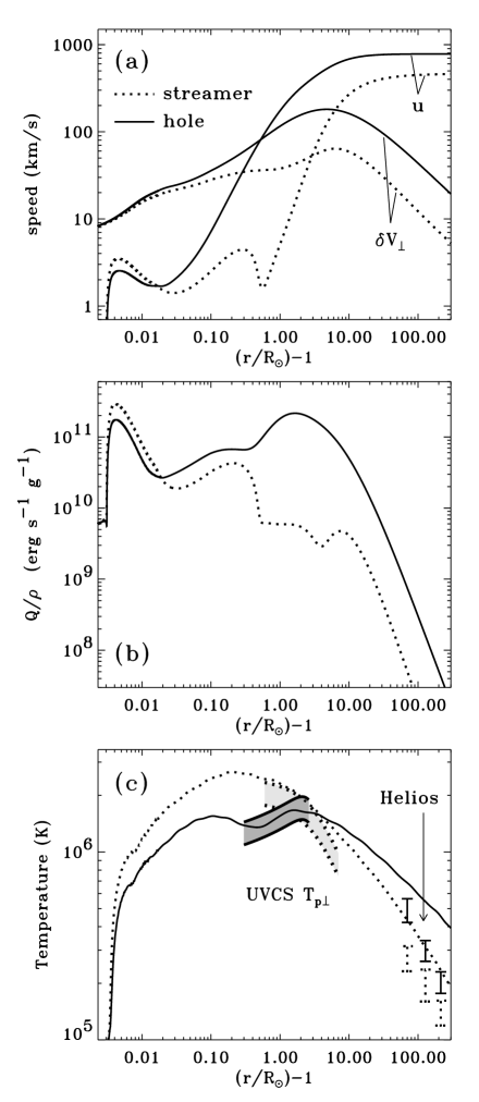
Figure 2: In all panels, solid lines represent the coronal-hole flux tube (fast wind) and dotted lines represent the streamer-edge flux tube (slow wind). (a) Outflow speed $u$ and 1D transverse Alfvén wave amplitude $\langle\delta V_{\perp}\rangle$ vs.  height above the photosphere. (b) Heating rates per unit mass. (c) Estimated one-fluid temperatures corresponding to the heating rates in (b). UVCS-derived proton temperatures and in-situ Helios one-fluid temperatures are shown for comparison (see text for references).

Figure 2b gives the derived heating rate—expressed as the energy flux density $Q$ per unit mass density $\rho$—for the two flux tube models. The slowly-varying ratio $Q/\rho$ is plotted for convenience, because $Q$ itself drops by more than 15 orders of magnitude between the transition region ($r\approx 1.003\,R_{\odot}$) and 1 AU. In some ways, though, the plot is deceiving because it seems as if the streamer flux tube is heated more than the polar-hole model only below $r\approx 1.02\,\,R_{\odot}$. In fact, $Q_{\rm streamer}>Q_{\rm hole}$ everywhere below $r\approx 1.4\,\,R_{\odot}$, but this is masked in the plot because $\rho_{\rm streamer}>\rho_{\rm hole}$. The heating rate is assumed to be equal to the energy cascade rate that has been derived for anisotropic MHD turbulence:

$$Q\,=\,\rho\,\frac{\langle Z_{-}\rangle^{2}\langle Z_{+}\rangle+\langle Z_{+}\rangle^{2}\langle Z_{-}\rangle}{4\ell_{\perp}}$$ (3)

(Hossain et al.  1995; Matthaeus et al.  1999; Dmitruk et al.  2001, 2002), where $\ell_{\perp}$ is a transverse outer-scale correlation length and Elsasser (1950) variables are used to distinguish between outwardly propagating waves ($Z_{-}$) and inwardly propagating waves ($Z_{+}$), with $Z_{\pm}\equiv\delta V\pm\delta B/\sqrt{4\pi\rho}$. The correlation length is assumed to expand with the transverse width of the flux tube (i.e., $\ell^{2}_{\perp}B={\rm{const;}}$ see Hollweg 1986), and its normalization is specified by Cranmer & van Ballegooijen (2005).

Figure 2c shows the result of integrating a one-fluid internal energy equation (e.g., eq. 3 of Leer & Holzer 1980) to compute the mean temperatures $T(r)$ that result from the heating rates discussed above. These results should be interpreted as preliminary because: (1) they are not the result of a self-consistent calculation of all fluid variables, and (2) a simple choice was made for the electron heat flux (i.e., $q_{e{\scriptscriptstyle\parallel}}=q_{\rm SH}/10$, where $q_{\rm SH}$ is the classical Spitzer-Härm value) in order to split the difference between the known strong conduction at low heights and the collisionless inhibition of $q_{{\scriptscriptstyle\parallel}e}$ at large heights. However, the overall trend in Figure 2c (i.e., the streamer being heated more at low heights, and less above the critical point, than the coronal hole) is likely to remain valid when the above approximations are corrected.

Several observations are also shown in Figure 2c, and the general agreement in the hole/streamer contrast lends credence to the overall validity of the approach outlined in this work. UVCS/SOHO measured H I Ly$\alpha$ resonance line profiles in the extended corona which provide a probe of proton velocity distributions. For off-limb observations, the line of sight samples directions that are mainly perpendicular to the $\sim$radial field lines, and the $1/e$ line width $V_{1/e}$ arises from two primary types of motion:

$$V_{1/e}^{2}\,=\,\frac{2k_{\rm B}T_{p\perp}}{m_{p}}+\langle\delta V_{\perp}\rangle^{2}\,\,.$$ (4)

The two terms on the right represent random thermal motions and unresolved transverse wave motions. Using measured values of $V_{1/e}$ and the modeled values of $\langle\delta V_{\perp}\rangle$ for the waves, the above equation was solved for the plotted $T_{p\perp}$. The UVCS curve for a solar-minimum coronal hole (dark gray) comes from an amalgam of data from Kohl et al.  (1997), Cranmer et al.  (1999), Esser et al.  (1999), Zangrilli et al.  (1999), and Antonucci et al.  (2000). The UVCS streamer data (light gray) came from Kohl et al.  (1997) and Strachan et al.  (2004). Also shown in Figure 2c are Helios data points which were computed by averaging together proton (Marsch et al.  1982) and electron (Pilipp et al.  1990) measurements, and isotropizing from bi-Maxwellian fits; i.e., taking $T\equiv(T_{{\scriptscriptstyle\parallel}}+2T_{\perp})/3$.

When examining predictions for the plasma temperatures in fast vs.  slow solar wind, it is worthwhile to compare with different, but potentially complementary ideas. Recently, Fisk (2003) and Schwadron & McComas (2003) discussed the origins of correlations between the eventual wind speed and observed properties of emerging loops in the low corona (see also the related footpoint diffusion model of Fisk & Schwadron 2001). Their prediction for there to be more basal coronal heating (and a higher mass flux) in the slow wind seems to be in accord with the results shown in Figure 2 (see also Matthaeus et al., these proceedings). There still seems to be a disconnect, though, between theories of coronal heating via flux emergence and theories that invoke magnetic footpoint shaking (which in turn generates waves). The relative contributions of these processes in various coronal regions needs to be quantified further.

6 Proton vs.  electron heating

The above analysis did not account explicitly for differences between heating the various particle species in the plasma. Even in a perfectly “collisionally coupled” plasma, there can be macroscopic dynamical consequences depending on how the energy is deposited into protons, electrons, and possibly heavy ions as well.

Hansteen & Leer (1995) demonstrated these effects for a 1D solar wind model: when all of the heat goes into electrons, there is substantially more downward conduction compared to a proton-heated model. An electron-heated wind thus has a lower mid-corona temperature and a lower wind speed than a proton-heated wind. A 2D simulation of streamers by Endeve et al.  (2004) showed that the stability of closed-field regions is closely related to this kinetic partitioning of heat. When protons are heated strongly, the modeled streamers become unstable to the ejection of massive plasmoids; when the electrons are heated, the streamers are stable. Any sufficiently predictive model of fast and slow solar wind must take these effects into account (see also Cranmer & van Ballegooijen 2003).

7 Conclusions and Future Missions

Our understanding of the dominant physics of solar wind acceleration has progressed rapidly in the SOHO era, and many of the insights embedded in the above analysis would not have been possible without SOHO. In particular, the strong preferential heating and acceleration of heavy ions seen in coronal holes by UVCS has sharpened theoretical efforts to understand kinetic energy deposition in the collisionless extended corona (see reviews by Axford et al.  1999; Hollweg & Isenberg 2002; Cranmer 2002a; Marsch 2004).

Despite these advances, the diagnostic capabilities of the SOHO instruments were limited and the most fundamental questions have not yet been answered. If the kinetic properties of additional ions were to be measured in the extended corona (i.e., a wider sampling of charge/mass combinations) we could much better constrain the specific kinds of waves that are present as well as the specific collisionless damping modes (Cranmer 2001, 2002b). Measuring the coronal electron temperature above $\sim$1.5 $R_{\odot}$ (never done directly before) would allow us to determine the bulk-plasma heating rate in different solar wind structures, thus putting the firmest ever constraints on models of why the fast/slow wind is fast/slow. Measuring non-Maxwellian velocity distributions of electrons and positive ions would allow us to test specific models of MHD turbulence, cyclotron resonance, and velocity filtration. New capabilities such as these would be enabled by greater photon sensitivity, an expanded wavelength range, and the use of measurements that heretofore have only been utilized in a testing capacity (e.g., Thomson-scattered H I Ly$\alpha$ to obtain $T_{e}$). Spectroscopy is key for the above measurements—especially in combination with coronagraph occultation—in order to measure detailed plasma properties out into the wind’s acceleration region (see also Kohl et al., these proceedings).

This work is supported by NASA under grants NAG5-11913, NAG5-10996, NNG04GE77G, and NNG04GE84G to the Smithsonian Astrophysical Observatory, by Agenzia Spaziale Italiana, and by the Swiss contribution to ESA’s PRODEX program.

References

- Blah (1999) Antonucci, E., et al., 2000, Solar Phys., 197, 115
- Blah (1999) Arge, C. N., Pizzo, V. J., 2000, JGR, 105, 10465
- Blah (1999) Axford, W. I., 1977, in Study of Travelling Interplanetary Phenomena (Dordrecht: Reidel), 145
- Blah (1999) Axford, W. I., et al., 1999, Space Sci. Rev., 87, 25
- Blah (1999) Axford, W. I., Newman, R. C., 1967, ApJ, 147, 230
- Blah (1999) Banaszkiewicz, M., et al., 1998, A&A, 337, 940
- Blah (1999) Bravo, S., Stewart, G. A., 1997, ApJ, 489, 992
- Blah (1999) Chen, Y., Hu. Y.-Q., 2002, Ap. Space Sci., 282, 447
- Blah (1999) Cranmer, S. R., 2001, JGR, 106, 24937
- Blah (1999) Cranmer, S. R., 2002a, Space Sci. Rev., 101, 229
- Blah (1999) Cranmer, S. R., 2002b, in SOHO–11: From Solar Min to Max, ESA SP–508, 361 (arXiv astro–ph/0209301)
- Blah (1999) Cranmer, S. R., et al., 1999, ApJ, 511, 481
- Blah (1999) Cranmer, S. R., van Ballegooijen, A. A., 2003, ApJ, 594, 573
- Blah (1999) Cranmer, S. R., van Ballegooijen, A. A., 2005, ApJ Suppl., 156, 265
- Blah (1999) Dmitruk, P., et al., 2001, ApJ, 548, 482
- Blah (1999) Dmitruk, P., et al., 2002, ApJ, 575, 571
- Blah (1999) Elsasser, W. M., 1950, Phys. Rev., 79, 183
- Blah (1999) Endeve, E., Holzer, T. E., Leer, E., 2004, ApJ, 603, 307
- Blah (1999) Esser, R., et al., 1999, ApJ, 510, L63
- Blah (1999) Feldman, W. C., et al., 1976, JGR, 81, 5054
- Blah (1999) Fisk, L. A., 2003, JGR, 108 (A4), 1157, doi:10.1029/ 2002JA009284
- Blah (1999) Fisk, L. A., Schwadron, N. A., 2001, ApJ, 560, 425
- Blah (1999) Gosling, J. T., 1996, Ann. Rev. Astron. Ap., 34, 35
- Blah (1999) Habbal, S. R., Woo, R., 2001, ApJ, 549, L253
- Blah (1999) Hansteen, V. H., Leer, E., 1995, JGR, 100, 21577
- Blah (1999) Hartle, R. E., Sturrock, P. A., 1968, ApJ, 151, 1155
- Blah (1999) Heinemann, M., Olbert, S., 1980, JGR, 85, 1311
- Blah (1999) Hick, P., et al., 1995, GRL, 22, 643
- Blah (1999) Hollweg, J. V., 1986, JGR, 91, 4111
- Blah (1999) Hollweg, J. V., Isenberg, P. A., 2002, JGR, 107 (A7), 1147, doi:10.1029/2001JA000270
- Blah (1999) Holzer, T. E., Leer, E., 1980, JGR, 85, 4665
- Blah (1999) Holzer, T. E., Leer, E., 1997, in 5th SOHO Workshop, ESA SP–404, 65
- Blah (1999) Hossain, M., et al., 1995, Phys. Fluids, 7, 2886
- Blah (1999) Hundhausen, A. J., 1972, Coronal Expansion and Solar Wind (Springer-Verlag)
- Blah (1999) Isenberg, P. A., Hollweg, J. V., 1982, JGR, 87, 5023
- Blah (1999) Kohl, J. L., et al., 1997, Solar Phys., 175, 613
- Blah (1999) Kopp, R. A., Holzer, T. E., 1976, Solar Phys., 49, 43
- Blah (1999) Kovalenko, V. A., 1978, Geomag. Aeronom., 18, 529
- Blah (1999) Kovalenko, V. A., 1981, Solar Phys., 73, 383
- Blah (1999) Krieger, A. S., et al., 1973, Solar Phys., 29, 505
- Blah (1999) Leer, E., Holzer, T. E., 1980, JGR, 85, 4681
- Blah (1999) Leer, E., et al., 1982, Space Sci. Rev., 33, 161
- Blah (1999) Levine, R. H., et al., 1977, JGR, 82, 1061
- Blah (1999) Liewer, P. C., et al., 2004, Solar Phys., 223, 209
- Blah (1999) Luhmann, J. G., et al., 2002, JGR, 107 (A8), doi: 10.1029/2001JA007550
- Blah (1999) Marsch, E. 2004, in SOHO–15: Coronal Heating, ESA SP–575, 186
- Blah (1999) Marsch, E., et al., 1982, JGR, 87, 52
- Blah (1999) Marsden, R. G., 2001, Ap. Space Sci., 277, 337
- Blah (1999) Matthaeus, W. H., et al., 1999, ApJ, 523, L93
- Blah (1999) Neugebauer, M., 1997, JGR, 102, 26887
- Blah (1999) Neugebauer, M., et al., 1998, JGR, 103, 14587
- Blah (1999) Nisenson, P., et al., 2003, ApJ, 587, 458
- Blah (1999) Noci, G., 1973, Solar Phys., 28, 403
- Blah (1999) Nolte, J. T., et al., 1976, Solar Phys., 46, 303
- Blah (1999) Parker, E. N., 1958, ApJ, 128, 664
- Blah (1999) Pilipp, W. G., et al., 1990, JGR, 95, 6305
- Blah (1999) Pneuman, G. W., 1980, A&A, 81, 161
- Blah (1999) Poduval, B., Zhao, X. P., 2004, JGR, 109, A08102, doi:10.1029/2004JA010384
- Blah (1999) Schwadron, N. A., McComas, D. J., 2003, ApJ, 599, 1395
- Blah (1999) Sittler, E. C., Jr., Guhathakurta, M., 1999, ApJ, 523, 812
- Blah (1999) Spruit, H. C., 1981, A&A, 98, 155
- Blah (1999) Strachan, L., et al., 2002, ApJ, 571, 1008
- Blah (1999) Strachan, L., et al., 2004, in SOHO–15: Coronal Heating, ESA SP–575, 148
- Blah (1999) Suess, S. T., 1982, ApJ, 259, 880
- Blah (1999) Tu, C.-Y., et al., 2005, Science, 308, 519
- Blah (1999) Vásquez, A. M., et al., 2003, ApJ, 598, 1361
- Blah (1999) Velli, M., 2001, Ap. Space Sci., 277, 157
- Blah (1999) Wang, Y.-M., 1994, ApJ, 437, L67
- Blah (1999) Wang, Y.-M., Sheeley, N. R., Jr., 1990, ApJ, 355, 726
- Blah (1999) Wang, Y.-M., Sheeley, N. R., Jr., 1991, ApJ, 372, L45
- Blah (1999) Wang, Y.-M., et al., 2000, JGR, 105, 25133
- Blah (1999) Wilcox, J. M., 1968, Space Sci. Rev., 8, 258
- Blah (1999) Zangrilli, L., et al., 1999, A&A, 342, 592
- Blah (1999) Zirker, J. B. (ed.) 1977, Coronal Holes and High-Speed Wind Streams (Colorado Assoc. Univ. Press)