Tracing Galaxy Formation with Stellar Halos I: Methods

Abstract

If the favored hierarchical cosmological model is correct, then the Milky Way system should have accreted $\sim 100-200$ luminous satellite galaxies in the past $\sim 12$ Gyr. We model this process using a hybrid semi-analytic plus N-body approach which distinguishes explicitly between the evolution of light and dark matter in accreted satellites. This distinction is essential to our ability to produce a realistic stellar halo, with mass and density profile much like that of our own Galaxy, and a surviving satellite population that matches the observed number counts and structural parameter distributions of the satellite galaxies of the Milky Way. Our model stellar halos have density profiles which typically drop off with radius faster than those of the dark matter. They are assembled from the inside out, with the majority of mass ($\sim 80\%$) coming from the $\sim 15$ most massive accretion events. The satellites that contribute to the stellar halo have median accretion times of $\sim 9$ Gyr in the past, while surviving satellite systems have median accretion times of $\sim 5$ Gyr in the past. This implies that stars associated with the inner halo should be quite different chemically from stars in surviving satellites and also from stars in the outer halo or those liberated in recent disruption events. We briefly discuss the expected spatial structure and phase space structure for halos formed in this manner. Searches for this type of structure offer a direct test of whether cosmology is indeed hierarchical on small scales.

1. Introduction

There has been a long tradition of searching in the stellar halo of our Galaxy for signatures of its formation. Stars in the halo provide an important avenue for testing theories of galaxy formation because they have long orbital time periods, have likely suffered little from dissipation effects, and tend to inhabit the outer regions of the Galaxy where the potential is relatively smooth and slowly evolving. The currently favored Dark Energy + Cold Dark Matter ($\Lambda$CDM) model of structure formation makes the specific prediction that galaxies like the Milky Way form hierarchically, from a series of accretion events involving lower-mass systems. This leads naturally to the expectation that the stellar halo should be formed primarily from disrupted, accreted systems. In this work, we develop an explicit, cosmologically-motivated model for stellar halo formation using a hybrid N-body plus semi-analytic approach. Set within the context of $\Lambda$CDM, we use this model to test the general consistency of the hierarchical formation scenario for the stellar halo and to provide predictions for upcoming surveys aimed at probing the accretion history of the Milky Way and nearby galaxies.

In a classic study, Eggen, Lynden-Bell, & Sandage (1962) used proper motions and radial velocities of 221 dwarfs to show that those with lower metallicity (i.e. halo stars) tended to move on more highly eccentric orbits. They interpreted this trend as a signature of formation of the lower metallicity stars during a rapid radial collapse. In contrast, Searle & Zinn (1978) suggested that the wide range of metallicites found in a sample of 19 globular clusters at a variety of Galactocentric radii instead indicated that the Galaxy formed from the gradual agglomeration of many sub-galactic sized pieces. A recent analysis of 1203 metal-poor Solar neighborhood stars, selected without kinematic bias (Chiba & Beers, 2000), points to the truth being some combination of these two pictures: this sample contained a small concentration of very low metallicity stars on highly eccentric orbits (reminiscent of Eggen, Lynden-Bell & Sandage’s, 1962 work) but otherwise showed no correlation of increasing orbital eccentricity with decreasing metallicity.

In the last decade, much more direct evidence for the lumpy build-up of the Galaxy has emerged in the form of clumps of stars in phase-space (and, in some cases, metallicity) both relatively nearby (Majewski, Munn, & Hawley, 1996; Helmi, White, de Zeeuw, & Zhao, 1999) and at much larger distances. The most striking example in the latter category is the discovery of the Sagittarius dwarf galaxy (Ibata, Gilmore, & Irwin, 1994; Ibata, Gilmore & Irwin, 1995) — hereafter Sgr — and its associated trails of debris (see Majewski et al., 2003, for an overview of the many detections) which have now been traced entirely around the Galaxy (Ibata et al., 2001; Majewski et al., 2003). Large scale surveys of the stellar halo are now underway (Majewski, Ostheimer, Kunkel, & Patterson, 2000; Morrison et al., 2000; Yanny et al., 2000; Ivezić et al., 2000; Newberg et al., 2002), and have uncovered additional structures, not associated with Sgr (Newberg et al., 2003; Martin et al., 2004; Rocha-Pinto et al., 2004). Moreover, recent advances in instrumentation are now permitting searches for and discoveries of analogous structures around other galaxies in the form of overdensities in integrated light (Shang et al., 1998; Zheng et al., 1999; Forbes et al., 2003; Pohlen et al., 2003) or, in the case of M31, star counts (Ibata et al., 2001; Ferguson et al., 2002; Zucker et al., 2004). Given this plethora of discoveries, there can be little doubt that the accretion of satellites has been an important contributor to the formation of our and other stellar halos. In addition, both theoretical (Abadi et al., 2003; Brook et al., 2005a; Robertson et al., 2005) and observational (Gilmore, Wyse, & Norris, 2002; Yanny et al., 2003; Ibata et al., 2003; Crane et al., 2003; Rocha-Pinto, Majewski, Skrutskie, & Crane, 2003; Frinchaboy et al., 2004; Helmi et al., 2005) work is beginning to suggest that some significant fraction of the Galactic disk could also have been formed this way.

All of the above discoveries are in qualitative agreement with the expectations of hierarchical structure formation (Peebles, 1965; Press & Schechter, 1974; Blumenthal et al., 1984). As the prevailing variant of this picture, $\Lambda$CDM is remarkably successful at reproducing a wide range of observations, especially on large scales (e.g. Eisenstein et al., 2005; Maller et al., 2005; Tegmark et al., 2004; Spergel et al., 2003; Percival et al., 2002). On sub-galactic scales, however, the agreement between theory and observation is not as obvious (e.g. Simon et al., 2005; Kazantzidis et al., 2004; D’Onghia & Burkert, 2004). Indeed, the problems explaining galaxy rotation curve data, dwarf galaxy counts, and galaxy disk sizes have lead some to suggest modifications to the standard paradigm, including an allowance for warm dark matter (e.g. Sommer-Larsen et al., 2004), early-decaying dark matter (Kaplinghat, 2005), or non-standard inflation (Zentner & Bullock, 2002, 2003). These modifications generally suppress fluctuation amplitudes on small scales, driving sub-galactic structure formation towards a more monolithic, non-hierarchical collapse. These issues bring to sharper focus a fundamental question in cosmology today: is structure formation truly hierarchical on small scales? Stellar halo surveys offer powerful data sets for directly answering this question.

Numerical simulations of individual satellites disrupting about parent galaxies can in many cases provide convincing similarities to the observed phase-space lumps. These models allow the observations to be interpreted in terms of the mass and orbit of the progenitor satellite (e.g., Velazquez & White, 1995; Johnston, Spergel, & Hernquist, 1995; Johnston, Sigurdsson, & Hernquist, 1999; Johnston et al., 1999; Helmi & White, 2001; Helmi et al., 2003; Law, Johnston & Majewski, 2004), and even the potential of the galaxy in which it is orbiting (Johnston, Zhao, Spergel, & Hernquist, 1999; Murali & Dubinski, 1999; Ibata et al., 2001; Ibata et al., 2004; Johnston, Law & Majewski, 2005). Nevertheless, a true test of hierarchical galaxy formation will require robust predictions for the frequency and character of the expected phase space structure of the halo.

Going beyond qualitative statements to model the full stellar halo (including substructure) within a cosmological context is non-trivial. The largest contributor of substructure to our own halo is Sgr, estimated to have a currently-bound mass of order $3\times 10^{8}M_{\odot}$ (Law, Johnston & Majewski, 2004). Even the highest resolution cosmological N-body simulations would not resolve such an object with more than a few hundred particles, which would permit only a poor representation of the phase-space structure of its debris (see Helmi, White, & Springel, 2003, for an example of what can currently be done in this field). Such simulations are computationally intensive, so the cost of examining more than a handful of halos is prohibitive and it is difficult to make statements about the variance of properties of halos that might be seen in a large sample of galaxies. Moreover, such simulations in general only follow the dark matter component of each galaxy not the stellar component. In their studies of thick disk and inner halo formation, Brook and collaborators (Brook et al., 2003, 2004a, 2004b, 2005a, 2005b) have modeled the stellar components directly by simulating the evolution of individual galaxies as isolated spheres of dark matter and gas with small-scale density fluctuations superimposed to account for the large-scale cosmology. However, their sample size remains small and, though they are able to make general statements about the properties of their stellar halos, their resolution would prohibit a detailed phase-space analysis.

An alternative is to take an analytic or semi-analytic approach to halo building (e.g. Bullock, Kravtsov, & Weinberg, 2001; Johnston, Sackett, & Bullock, 2001; Taylor, 2004). This allows the production of many halos, and the potential of including prescriptions to follow the stars separately from the dark matter. However, such techniques use only approximate descriptions of the dynamics and are unable to follow the fine details of the phase-space structure accurately.

In this study we develop a hybrid scheme, which draws on the strengths of each of the former techniques to build high resolution, full phase-space models of a statistical sample of stellar halos. Our approach is to vastly decrease the computational cost of a full cosmological simulation by modeling only those accretion events that contribute directly to the stellar halo in detail with N-body simulations, and to represent the rest of the galaxy with smoothly-evolving analytic functions. The baryonic component of each contributing event is followed using semi-analytic prescriptions.

The purpose of this paper is to describe our method, its strengths and limitations (§2), present the results of tests of the consistency of our models with general properties of galaxies and their satellite systems (§3) and outline some implications (§4). We summarize the conclusions in §5. In further work we will go on to compare the full phase-space structure of our halos in detail to observations and to examine the evolution of dark and light matter in satellite galaxies after their accretion.

2. Methods

Our methods can be broadly separated into: (I) a simulation phase, which follows the phase-space evolution of the dark matter; and (II) a prescription phase, which embeds a stellar mass with each dark matter particle. Specifically:

Phase I: Simulations

1. We generate merger trees for our parent galaxies using the method outlined in Somerville & Kolatt (1999) based on the Extended-Press-Schechter (EPS) formalism (Lacey & Cole, 1993, — see §2.1)).

2. For each event in step IA, we run a high-resolution N-body simulation that tracks the evolution of the dark matter component of a satellite disrupting within an analytic, time-dependent, parent galaxy + host halo potential (see §2.2).

Phase II: Prescriptions

1. We follow the gas accretion history of each satellite prior to falling into the parent and track its star-formation rate using cosmologically-motivated, semi-analytic prescriptions (see §2.3).

2. We embed the stellar components generated in step IIA within each dark matter satellite by assigning a variable mass-to-light ratio to every particle that is tracked in the (Phase I) N-body simulations (see §2.4).

We consider the two-phase approach a necessary and acceptable simplification since it allows us to separate well-understood and justified approximations in Phase I from prescriptions that can be adjusted and refined during Phase II. In addition, this separation allows us to save computational time and use just one set of dark matter simulations to explore the effect of varying the details of how baryons are assigned to each satellite. A more complete discussion of the strengths and limitations of our scheme is given in §2.5.

2.1. Cosmological Framework

Throughout this work we assume a $\Lambda$CDM cosmology with $\Omega_{\rm m}=0.3$, $\Omega_{\rm\Lambda}=0.7$, $\Omega_{\rm b}h^{2}=0.024$, $h=0.7$, and $\sigma_{8}=0.9$. The implied baryon fraction is $\Omega_{b}/\Omega_{\rm m}=0.16$.

We focus on the formation of stellar halos for “Milky-Way” type galaxies. In all cases our $z=0$ host dark matter halos have virial masses $M_{\rm vir,0}=1.4\times 10^{12}M_{\odot}$, corresponding virial radii $R_{\rm vir,0}=282$ kpc, and virial velocities $V_{\rm vir}=144{\rm km}\,{\rm s}^{-1}$. The quantities $M_{\rm vir}$ and $R_{\rm vir}$ are related by

$$M_{\rm vir}=\frac{4\pi}{3}\rho_{\rm M}(z)\Delta_{\rm vir}(z)R_{\rm vir}^{3},$$ (1)

where $\rho_{\rm M}$ is the average matter density of the Universe and $\Delta_{\rm vir}$ is the “virial overdensity”. In the cosmology considered here, $\Delta_{\rm vir}(z=0)\simeq 337$, and $\Delta_{\rm vir}\rightarrow 178$ at $z\lower 2.58334pt\vbox{\hbox{$\buildrel\textstyle>\over{\sim}\ $}}1$ (Bryan & Norman, 1998). The virial velocity is defined as $V_{\rm vir}\equiv\sqrt{GM_{\rm vir}/R_{\rm vir}}$.

We generate a total of eleven random realizations of stellar halos. General properties of all eleven are summarized in Table 1. Any variations in our results for stellar halos among these are determined by differences in their accretion histories. In all subsequent figures we present results for four stellar halos (1,2,6, and 9) chosen to span the range of properties seen in our full sample.

2.1.1 Semi-analytic accretion histories

We track the mass accretion and satellite acquisition of each parent galaxy by constructing merger trees using the statistical Monte Carlo method of Somerville & Kolatt (1999) based on the EPS formalism (Lacey & Cole, 1993). This method gives us a record of the the masses and accretion times of all satellite halos and hence allows us to follow the mass accretion history of each parent as a function of lookback time. We explicitly note all satellites more massive than $M_{\rm min}=5\times 10^{6}M_{\odot}$ and treat all smaller accretion events as diffuse mass accretion. Column 2 of Table 1 lists the total number of such events for each simulated halo. For further details see Lacey & Cole (1993); Somerville & Kolatt (1999); Zentner & Bullock (2003). Four examples of the cumulative mass accretion histories of parent galaxies generated in this manner are shown by the (jagged) solid lines in Figure 1.

2.1.2 Satellite orbits

Upon accretion onto the host, each satellite is assigned an initial orbital energy based on the range of binding energies observed in cosmological simulations (Klypin et al., 1999). This is done by placing each satellite on an initial orbit of energy equal to the energy of a circular orbit of radius $R_{\rm circ}=\eta R_{\rm vir}$, with $\eta$ drawn randomly from a uniform distribution on the interval $[0.4,0.8]$. Here $R_{\rm vir}$ is the virial radius of the host halo at the time of accretion. We assign each subhalo an initial specific angular momentum $J=\epsilon J_{\rm circ}$, where $J_{\rm circ}$ is the specific angular momentum of the aforementioned circular orbit and $\epsilon$ is the orbital circularity, which takes a value between $0$ and $1$. We choose $\epsilon$ from the binned distribution shown in Figure 2 of Zentner & Bullock (2003), which was designed to match the cosmological N-body simulation results of Ghigna et al (1998), and is similar to the circularity distributions found in more recent N-body analyses (Zentner et al., 2004; Benson, 2005). Finally, the plane of the orbit is drawn from a uniform distribution covering the halo sphere.

2.1.3 Dark matter density distributions

We model all satellite and parent halos with the spherically averaged density profile of Navarro, Frenk & White (1996) (NFW):

$$\rho_{{}_{\rm NFW}(r)}=\rho_{\mathrm{s}}\left(\frac{r}{r_{\rm halo}}\right)^{-1}\left(1+\frac{r}{r_{\rm halo}}\right)^{-2},$$ (2)

where $r_{\rm halo}$ ($\equiv r_{s}$ in NFW) is the characteristic inner scale radius of the halo. The normalization, $\rho_{\mathrm{s}}$, is set by the requirement that the mass interior to $R_{\rm vir}$ be equal to $M_{\rm vir}$. The value of $r_{\rm halo}$ is usually characterized in terms of of the halo “concentration” parameter: $c\equiv R_{\rm vir}/r_{\rm halo}$. The implied maximum circular velocity for this profile occurs at a radius $r_{\rm max}\simeq 2.15r_{\rm halo}$ and takes the value $V_{\rm max}\simeq 0.466V_{\rm vir}F(c)$, where $F(c)=\sqrt{c/[\ln(1+c)-c/(1+c)]}$.

For satellites, we set the value of $c$ using the simulation results of Bullock et al. (2001) and the corresponding relationship between halo mass, redshift, and concentration summarized by their analytic model. The median $c$ relation for halos of mass $M_{\rm vir}$ at redshift $z$ is given approximately by

$$c\simeq 9.6\left(\frac{M_{\rm vir}}{10^{13}M_{\odot}}\right)^{-0.13}(1+z)^{-1},$$ (3)

although in practice we use the full analytic model discussed in Bullock et al. (2001).

For parent halos, we allow their concentrations to evolve self-consistently as their virial masses increase, as has been seen in the N-body simulations of Wechsler et al. (2002). Rather than represent the halo growth as a series of discrete accretion events, we smooth over the Monte Carlo EPS merger tree by fitting the following functional form to the Monte Carlo mass accretion history for each halo:

$$M_{\rm vir}(a) = M_{\rm vir}(a_{0})\exp\left[-2a_{c}\left(\frac{a_{0}}{a}-1\right)\right].$$ (4)

Here $a\equiv(1+z)^{-1}$ is the expansion factor, and $a_{c}$ is the fitting parameter, corresponding to the value of the expansion factor at a characteristic “epoch of collapse”. Wechsler et al. (2002) demonstrated that the value of $a_{c}$ connects in a one-to-one fashion with the halo concentration parameter (Wechsler et al., 2002):

$$c(a)=5.1{a\over a_{c}}.$$ (5)

Halos that form earlier (smaller $a_{c}$’s) are more concentrated.

Example fits to four of our halo mass accretion histories are shown by the smooth solid lines in Figure 1. The $a_{c}$ values for each of the halos in this analysis are listed in the third column of Table 1. Typical host halos in our sample have $c\simeq 14$ at $z=0$, scale radii $r_{\rm halo}\simeq 20$kpc, and maximum circular velocities $V_{\rm max}\simeq 190{\rm km}\,{\rm s}^{-1}$.

2.2. N-body simulations of dark matter evolution

Having determined the mass, accretion time and orbit of each satellite (§2.1.1 and §2.1.2), and the evolution the potential into which it is falling (§2.1.3), we next run individual N-body simulations to track the dynamical evolution of each satellite halo separately. We follow only those that contain a significant stellar component (see §2.3 below). In practice, this restricts our analysis to satellite halos more massive than $M_{\rm vir}\lower 2.58334pt\vbox{\hbox{$\buildrel\textstyle>\over{\sim}\ $}}10^{8}M_{\odot}$ — the number of such satellites infalling into each parent is listed in column 5 of Table 1. Based on our star-formation prescription discussed in §2.3, systems smaller than this never contain an appreciable number of stars and thus don’t contribute significantly to the stellar halo.

2.2.1 The parent galaxy potential

The parent galaxy is represented by a three-component bulge/disk/dark halo potential which we allow to evolve with time as the halo accretes mass. The (spherically-symmetric) dark halo potential at each epoch $a$ is given by the NFW potential generated by the dark matter distribution in equation (2)

$$\Phi_{\rm halo}(r)=-{GM_{\rm halo}\over r_{\rm halo}}{1\over(r/r_{\rm halo})}\ln\left({r\over r_{\rm halo}}+1\right),$$ (6)

equation where $M_{\rm halo}=M_{\rm halo}(a)$ and $r_{\rm halo}=r_{\rm halo}(a)$ are the instantaneous mass and length scales of the halo respectively. The halo mass scale is related to the virial mass via

$$M_{\rm halo} = {M_{\rm vir}\over\ln(c+1)-c/(c+1)}.$$ (7)

The disk and bulge are assumed to grow in mass and scale with the halo virial mass and radius:

$$\Phi_{\rm disk}(R,Z)=-{GM_{\rm disk}\over\sqrt{R^{2}+\left(R_{\rm disk}+\sqrt{Z^{2}+Z_{\rm disk}^{2}}\right)^{2}}},$$ (8)

$$\Phi_{\rm sphere}(r)=-{GM_{\rm sphere}\over r+r_{\rm sphere}},$$ (9)

where $M_{\rm disk}(a)=1.0\times 10^{11}(M_{\rm vir}/M_{\rm vir,0})M_{\odot}$, $M_{\rm sphere}(a)=3.4\times 10^{10}(M_{\rm vir}/M_{\rm vir,0})M_{\odot}$, $R_{\rm disk}=6.5(r_{\rm vir}/r_{\rm vir,0})$ kpc, $Z_{\rm disk}=0.26(r_{\rm vir}/r_{\rm vir,0})$ kpc and $r_{\rm sphere}=0.7(r_{\rm vir}/r_{\rm vir,0})$ kpc.

2.2.2 Satellite initial conditions

We use $10^{5}$ particles to represent the dark matter in each accreted satellite. Particles are initially distributed as an isotropic NFW model, with mass and scale chosen as described in §2.1.2. The phase-space distribution function is derived by integrating over the density and potential distributions

$$f(\epsilon)={1\over 8\pi^{2}}\left[\int_{0}^{\epsilon}{d^{2}\rho\over d\Psi^{2}}{d\Psi\over\sqrt{\epsilon-\Psi}}+\frac{1}{\sqrt{\epsilon}}\left(\frac{d\rho}{d\Psi}\right)_{\Psi=0}\right].$$ (10)

with $\rho=\rho_{{}_{\rm NFW}}$ and where $\Psi=-\Phi_{{}_{\rm NFW}}+\Phi_{0}$ is the relative potential (such that $\Psi\rightarrow 0$ as $r\rightarrow\infty$) and $\epsilon=\Psi-v^{2}/2$ is the relative energy (see Binney & Tremaine, 1987, for discussion). This distribution function is used (in tabulated form) to generate a random realization. This ensures a stable satellite configuration — initial conditions generated by instead assuming a local Maxwellian velocity distribution have been shown to evolve (Kazantzidis, Magorrian, & Moore, 2004). Given $f(\epsilon)$, the differential energy distribution follows in a straightforward manner from the density of states, $g(\epsilon)$,

$$\frac{dM}{d\epsilon}=f(\epsilon)g(\epsilon),\quad g(\epsilon)\equiv 16\pi^{2}\int_{0}^{r_{\epsilon}}\sqrt{2(\Psi-\epsilon)}r^{2}dr,$$ (11)

where $r_{\epsilon}$ is the largest energy that can be reached by a star of relative energy $\epsilon$. The differential energy distribution for our initial halo is shown by the solid histogram in Figure 2. We see that the majority of the (dark matter) material in an infalling satellite is quite loosely bound.

Rather than generating a unique $f(\epsilon)$ and particle distribution for each satellite in each accretion history, a single initial conditions file with unit mass and scale, and outer radius $R_{\rm out}=35r_{\rm halo}$ ($=35$ in our units) is used for all simulations with masses and scales appropriately rescaled for each run. Since all of our accreted satellites have concentrations $c<35$, our set up effectively allows each accreted satellite’s mass profile to extend beyond its virial radius for several scale lengths. We do not expect this simplification to significantly affect our results because the the light matter is always embedded at the very central regions of the halo ($r_{\star}\lower 2.58334pt\vbox{\hbox{$\buildrel\textstyle<\over{\sim}\ $}}r_{\rm halo}$) and the outer material is always quickly stripped away from the outer parts of the halos upon accretion.

In §2.4 we discuss our method of “embedding” star particles within the cores the accreted satellite dark halos.

2.2.3 Satellite evolution

The mutual interactions of the satellite particles are calculated using a basis function expansion code (Hernquist & Ostriker, 1992). The initial conditions file for the satellite is allowed to relax in isolation for ten dynamical times using this code to confirm stability. For each accretion event a single simulation is run, following the evolution of the relaxed satellite under the influence of its own and the parent galaxy’s potential, for the time since it was accreted (as generated by methods in §2.1.1) along the orbit chosen at random from the distribution discussed in §2.1.2. (Note that simulations of satellite accretions in static NFW potentials using this code produced results identical to those reported in Hayashi et al., 2003)

Using this approach, the satellites are not influenced by each other, other than through the smooth growth of the parent galaxy potential. Nor does the parent galaxy react to the satellite directly. In order to mimic the expected decay of the satellite orbits due to dynamical friction (i.e. the interaction with the parent), we include a drag term on all particles within two tidal radii $r_{\rm tide}$ of the satellite’s center, of the form proposed by Hashimoto, Funato, & Makino (2003) and modified for NFW hosts by Zentner & Bullock (2003). This approach includes a slight modification to the standard Chandrasekhar dynamical friction formula (e.g. Binney & Tremaine, 1987). The tidal radius $r_{\rm tide}$ is calculated from the instantaneous bound mass of the satellite $m_{\rm sat}$, the distance $r$ of the satellite to the center of the parent galaxy and the mass of the parent galaxy within that radius $M_{r}$ as $r_{\rm tide}=r(m_{\rm sat}/M_{r})^{1/3}$.

2.2.4 Increasing phase-space resolution with test particles

In this study, we are most interested in following the phase-space evolution of the stellar material associated with each satellite. This is assumed to be embedded deep within each dark matter halo (see §2.4) — typically only of order $10^{4}$ of the N-body particles in each satellite have any light associated with them at all. In order to increase the statistical accuracy our analysis we sample the inner 12% of the energy distribution with an additional $1.2\times 10^{5}$ test particles. This does not increase the dynamic range our simulation, but does allow us to more finely resolve the low surface brightness features we are interested in with only a modest increase in computational cost: we gain a factor of 10 in particle resolution with an increase of $\sim$25% in computing time. In this paper, we have used test particles only in generating the images shown in Figures 13 - 16.

2.3. Following the satellites’ baryonic component

We follow each satellite’s baryonic component using the expected mass accretion history of each satellite halo (prior to falling into the parent galaxy) in order to track the inflow of gas. The gas mass is then used to determine the instantaneous star formation rate and to track the buildup of stars within each halo. The physics of galaxy formation is poorly understood, and any attempt to model star formation and gas inflow into galaxies (whether semi-analytic or hydrodynamic) necessarily require free parameters. Our own prescription requires three ”free” parameters: $z_{\rm re}$, the redshift of reionization (see §2.3.1); $f_{\rm gas}$, the fraction of baryonic material in the form of cold gas (i.e. capable of forming stars) that remains bound to each satellite at accretion (see §2.3.2); and $t_{\star}$, the globally-averaged star formation timescale (see §2.3.3).

In the following subsections we describe how these parameters enter into our prescriptions, and choose a value of $f_{\rm gas}$ consistent with observations. In §3 we go on to demonstrate that the observed characteristics of the stellar halo (e.g. its mass, and radial profile) and the Milky Way’s satellite system (e.g. their number and distribution in structural parameters) provide strong constraints on the remaining free parameters and hence the efficiency of star formation in low-mass dark matter halos in general.

2.3.1 Reionization

Any attempt to model stellar halo buildup within the context of $\Lambda$CDM must first confront the so-called “missing satellite problem” — the apparent over-prediction of low-mass halos compared to the abundance of satellite galaxies around the Milky Way and M31. For example, there are eleven know satellites of the Milky Way — nine classified as dwarf spheroidal and two as dwarf irregulars — yet numerical work predicts several hundred dark matter satellite halos in a similar mass range (Klypin et al., 1999; Moore et al., 1999). It is quite likely that our inventory of stellar satellites is not complete given the luminosity and surface brightness limits of prior searches (as the recent discovery of the Ursa Minor dwarf spheroidal demonstrates, see Willman et al., 2005), but incompleteness is not seen as a viable solution for a problem of this scale (see Willman et al., 2004, for a discussion).

The simplest solution to this problem is to postulate that only a small fraction of the satellite halos orbiting the Milky Way host an observable galaxy. In this work, we solve the missing satellite problem using the suggestion of Bullock, Kravtsov, & Weinberg (2000), which maintains that only the $\sim 10\%$ of low-mass galaxies ($V_{\rm max}<30{\rm km}\,{\rm s}^{-1}$) that had accreted a substantial fraction of their gas before the epoch of reionization host observable galaxies (see also Chiu et al., 2001; Somerville, 2002; Benson et al., 2002; Kravtsov et al., 2004). The key assumption is that after the redshift of hydrogen reionization, $z_{\rm re}$, gas accretion is suppressed in halos with $V_{\rm max}<50{\rm km}\,{\rm s}^{-1}$, and completely stopped in halos with $V_{\rm max}<30{\rm km}\,{\rm s}^{-1}$. These thresholds follow from the results of Thoul & Weinberg (1996) and Gnedin (2000) who used hydrodynamic simulations to show that gas accretion in low-mass halos is indeed suppressed in the presence of an ionizing background.

We also impose a low-mass cutoff for tracking galaxy formation in satellite halos with $V_{\rm max}<15{\rm km}\,{\rm s}^{-1}$. Two processes and one practical consideration motivate us to ignore galaxy formation in these tiny halos: first, photo-evaporation acts to eliminate any gas that was accreted before reionization in halos with $V_{\rm max}\lower 2.58334pt\vbox{\hbox{$\buildrel\textstyle<\over{\sim}\ $}}15{\rm km}\,{\rm s}^{-1}$ (Barkana & Loeb, 1999; Shaviv & Dekel, 2003); second, the cooling barrier below virial temperatures of $\sim 10^{4}$K (corresponding to $V_{\rm max}\sim 16{\rm km}\,{\rm s}^{-1}$) prevents any gas that could remain bound to these halos from cooling and forming stars (Kepner et al., 1997; Dekel & Woo, 2003); finally, even if we were to allow star formation in these systems, their contribution to the stellar halo mass would be negligible. Once we are more confident of our inventory of the lowest luminosity and lowest surface brightness satellites (Willman et al., 2004)of the Milky Way we should be able to confirm these physical arguments with observational constraints.

The epoch of reionization $z_{\rm re}$ determines the numbers of galaxies that have collapsed in each of the above $V_{\rm max}$ limits, and hence the number of luminous satellites that will be accreted, whether they disrupt to form the stellar halo or survive to form the Galaxy’s satellite system. We discuss limits on this parameter in §3.1.1.

2.3.2 Gas accretion following reionization

The virial mass of each satellite, $M_{\rm vir}^{\rm sat}$, at the time of its accretion, $a_{\rm ac}$, is set by our merger tree initial conditions (§2.1.1). We assume that each satellite halo has had a mass accumulation history set by Equation 4 up to the time of its merger into the “Milky Way” host, with $a_{0}=a_{\rm ac}$. After accretion, all mass accumulation onto the satellite is truncated (see §2.3.3). For massive satellites, $V_{\rm max}>50{\rm km}\,{\rm s}^{-1}$, we set $a_{c}$ in Equation 4 using the satellite’s mass-defined concentration parameter via Equation 5 (see Bullock et al., 2001; Wechsler et al., 2002). This provides a “typical” formation history for each satellite. For low-mass satellites, we are necessarily interested in where $a_{c}$ falls in the distribution of halo formation epochs because this determines the fraction of mass in place at reionization. Therefore, if $V_{\rm max}<50{\rm km}\,{\rm s}^{-1}$, we use the methods of Lacey & Cole (1993) in order to derive the fraction of the satellite’s mass that was in place at the epoch of reionization, $z_{\rm re}$, and use this to set the value of $a_{c}$. Given $a_{c}$ for each satellite, we determine the instantaneous accretion rate of dark matter $h(t)$ in to this system as a function of cosmic time via

$$h(t)=\frac{\mathrm{d}M_{\rm vir}^{\rm sat}}{{\mathrm{d}}t}.$$ (12)

In the absence of radiative feedback effects, cooling is extremely efficient in pre-merged satellites of the size we consider (see, e.g. Maller & Bullock, 2004). Therefore we expect the cold gas inflow rate to track the dark matter accretion rate, $h(t)$ — at least in the absence of the effects of reionization — and take it to be

$$Cf_{\rm gas}\,h(t-t_{\rm in}).$$ (13)

The time lag within $h(t)$ accounts for the finite time it takes for gas to settle into the center of the satellite after being accreted. We assume this occurs in roughly a halo orbital time at the virial radius: $t_{\rm in}=\pi R_{\rm h}/V_{\rm vir}\simeq 6\,{\rm Gyr}\,\,(1+z)^{-3/2}$. We have introduced the constant $C$ in order to account for the suppression of gas accretion in low-mass halos (as alluded to in §2.3.1). Before the epoch of reionization, we set $C=1$ for all galaxies. For systems with $V_{\rm max}>50{\rm km}\,{\rm s}^{-1}$, $C=1$ at all times. After reionization, $C=0$ in systems with $V_{\rm max}<30{\rm km}\,{\rm s}^{-1}$, and $C$ varies linearly in $V_{\rm max}$ between $0$ and $1$ if $V_{\rm max}$ falls between $30$ and $50{\rm km}\,{\rm s}^{-1}$ (see Thoul & Weinberg, 1996).

The fraction of mass in each satellite in the form of cold, accreting baryons, $f_{\rm gas}$, determines the total stellar mass plus cold gas mass associated with each dark matter halo. In what follows, we adopt $f_{\rm gas}=0.02$, which is an upper limit on the range of cold baryonic mass fraction in observed galaxies (Bell et al. 2003).

2.3.3 Star Formation

If we assume that cold gas forms stars over a timescale $t_{\star}$, then the evolution of stellar mass $M_{\star}$ and cold gas mass $M_{\rm gas}$ follows a simple set of equations:

$$\frac{\mathrm{d}M_{\star}}{\mathrm{d}t} = \frac{M_{\rm gas}}{t_{\star}},$$ (14)

$$\frac{\mathrm{d}M_{\rm gas}}{\mathrm{d}t} = -\frac{\mathrm{d}M_{\star}}{\mathrm{d}t}+Cf_{\rm gas}\,h(t-t_{\rm in}).$$ (15)

For simplicity, the star formation is truncated soon after each satellite halo is accreted onto the Milky Way host. Physically, this could result from gas loss via ram-pressure stripping from the background hot gas halo (Lin & Faber, 1983; Moore & Davis, 1994; Blitz & Robishaw, 2000; Maller & Bullock, 2004; Mayer et al., 2005). This model is broadly consistent with observations that demonstrate that the gas fraction in satellites of the Milky Way and Andromeda is typically far less than that in field dwarfs in the Local Group, as illustrated by the separation of the open (satellites) and filled (field dwarfs) symbols in Figure 3 (plotting data taken from Grebel, Gallagher, & Harbeck, 2003). Of course, this assumption is over-simplified, but it allows us to capture in general both the expectations of the hierarchical picture and the observational constraints. We note that this is likely a bad approximation for massive satellites, whose deep potential wells will tend to resist the effects of ram-pressure stripping. However, we expect that this will have little impact on our stellar halo predictions, since most of the stellar halo is formed from satellites that are accreted early and destroyed soon after.

The star formation timescale, $t_{\star}$ determines the star to cold gas fraction in each satellite upon accretion and, for a given value of $f_{\rm gas}$, total stellar luminosity associated with each surviving satellite and the stellar halo. We discuss limits on this parameter in §3.1.2.

2.4. Embedding baryons within the dark matter satellites

We model the evolution of a two-component population of stellar matter and dark matter in each satellite by associating stellar matter with the more tightly bound material in the halo. As discussed in §2.1.3, the mass profile of the satellite is assumed to take the NFW form. Mass-to-light ratios for each particle are picked based on the particle energy in order to produce a realistic stellar profile for a dwarf galaxy.

A phenomenologically-motivated approximation for the stellar distribution in dwarf galaxies is the spherically symmetric King profile (King 1962):

$$\rho_{\star}(r)=\frac{K}{x^{2}}\Bigg{(}\frac{\cos^{-1}(x)}{x}-\sqrt{1-x^{2}}\Bigg{)},\quad x\equiv\frac{1+(r/r_{\rm c})^{2}}{1+(r_{\rm t}/r_{\rm c})^{2}}.$$ (16)

The core radius is $r_{\rm c}$ and $r_{\rm t}$ is the tidal radius, where $\rho_{\star}(r>r_{\rm t})=0$. The normalization, $K$, is set by the average density of the satellite, determined by its mass (2.3.3) and size scales (discussed below).

For each satellite, we assume a stellar mass to light ratio of $M_{\star}/L_{\rm V}=2$, and use the stellar mass calculated in §2.3.3 in order to assign a median King core radius

$$r_{c}=160{\rm pc}\left(\frac{L_{\star}}{10^{6}L_{\odot}}\right)^{0.19},$$ (17)

where throughout $L_{\star}$ is assumed to be the V-band stellar luminosity. We allow scatter about the relation using a uniform logarithmic deviate between $-0.3\leq\Delta\log_{10}L\leq 0.3$. This slope and normalization was determined by least-square fit to the luminosity and core size correlation for the dwarf satellite data presented in Mateo (1998), and the scatter was determined by a “by-eye” comparison to the scatter in the data about the relation. Our adopted relation between $r_{c}$ and $L_{\star}$ is also consistent with the relevant projection of the fundamental plane for dwarf galaxies (e.g. Kormendy 1985). For all satellites we adopt $r_{\rm t}/r_{\rm c}=10.$

Assuming isotropic orbits for the stars and that the gravitational potential is completely dominated by the dark matter, the stellar energy distribution function corresponding to the King profile $f_{\star}(\epsilon)$ is determined by setting $\rho=\rho_{\star}$ and $\Psi=-\Phi_{{}_{\rm NFW}}+\Phi_{0}$ in equation (10). The mass-to-light ratio of a particle of energy $\epsilon$ is then simply $f_{\star}(\epsilon)/f(\epsilon)=(dM/d\epsilon)_{\star}/(dM/d\epsilon)$. Three examples are given Figure 2.

2.5. Limitations of our method

The main limitation of our method is that it only follows the smooth growth of the parent potential analytically — the satellite/satellite interactions and reaction of the parent to the satellite are not modeled self-consistently. Hence we do not anticipate following the evolution of the field or satellite particles during a major or even minor merger event with great accuracy. Given this limitation, we only simulate the accretion histories of halos generated from the Monte Carlo merger tree code that have not suffered a significant merger ($>$10 % of the parent halo mass) in the recent past ($<$7 Gyr) — 11 of the 20 accretion histories generated met this criterion. In addition, we consider results from simulations of accretion events that have occurred prior to the last significant merger to be less reliable. We label the halos used in this work 1-11. The five left-hand columns of Table 1 summarize the properties of the simulations run for each halo.

Even with these restrictions, we consider our study to be a useful approach for exploring substructure in galaxy halos because: (i) the highest surface brightness features in halos are likely to have come from recent events, whose debris has had a shorter time to phase-mix and/or be dispersed by oscillations in the parent galaxy potential; and (ii) substructure should be more readily detectable around spiral (rather than elliptical) galaxies because their stellar distributions are less extended — the existence of disks in spirals suggests that these are the ones the more quiescent accretion histories.

3. Results I: Tests of the Model

As outlined in §2.5, our method most accurately follows the phase-space evolution of debris from accretion events that occur during relatively quiescent times in a galaxy’s history (which we define as being after the last $>$10% merger event). In future work we concentrate on those events. In this paper, we analyze the results from simulations of the full accretion histories of our halos. While not accurate in following the phase-space properties of debris material from events occurring before the epoch of major merging, the fact that these systems are disrupted is predicted robustly, and we are able to record the time of disruption and the cumulative mass in those disrupted events as well.

In what follows, we first constrain the remaining free parameters $z_{\rm re}$ (§3.1.1) and $t_{\star}$ (§3.1.2) (with $f_{\rm gas}=0.02$), by requiring that the general properties of our surviving satellite populations are consistent with those of the Milky Way’s own satellites. We then go on to demonstrate that these parameter choices naturally produce the observed distributions in and correlations of the structural parameters of surviving satellites (see §3.2.1 and 3.2.2), as well as stellar halos with total luminosity and radial profiles consistent with the Milky Way (§3.2.3).

3.1. Primary constraints on parameters

3.1.1 Satellite number counts

As described in §2.3.1, we have chosen to solve the missing satellite problem by suppressing gas accretion in small halos after the epoch of reionization, $z_{\rm re}$, and suppressing gas accumulation all together in satellites smaller than $15{\rm km}\,{\rm s}^{-1}$. The number of satellites that host stars is then set by choosing $z_{\rm re}$. In the work presented in this paper, we assume that reionization occurred at a redshift $z_{\rm re}=10$ or at a lookback time of $13$Gyr. The fifth column of Table 1 gives the number of luminous satellites accreted over the lifetime of each halo and the sixth column gives the number of luminous satellites that survive disruption in each. (The numbers in brackets are for those events since the last $>$10% merger.) We see that our reionization prescription leads to agreement within a factor of $\sim 2$ with the number of satellites observed orbiting the Milky Way. Our results are roughly insensitive to this choice as long as $8\lower 2.58334pt\vbox{\hbox{$\buildrel\textstyle<\over{\sim}\ $}}z_{\rm re}\lower 2.58334pt\vbox{\hbox{$\buildrel\textstyle<\over{\sim}\ $}}15$.

3.1.2 Infalling satellite gas content

When reviewing the properties of Local Group dwarf galaxies it is striking that — with the notable exceptions of the Large and Small Magellanic Clouds (hereafter LMC and SMC) — satellites of the Milky Way and Andromeda galaxies are exceedingly gas-poor compared to their field counterparts (Mateo, 1998; Grebel, Gallagher, & Harbeck, 2003). Figure 3 emphasizes this point by plotting the V-band luminosity vs gas fraction from the compilation by Grebel, Gallagher, & Harbeck (2003) for satellites (open squares) and field dwarfs (filled squares). We see that field dwarfs tend to have $M_{HI}/L_{V}\simeq 0.3-3$, whereas satellite dwarfs have gas fractions $\sim 0.001-0.1$.

While our star formation model assumes that most of the gas in accreted dwarfs is lost shortly after a dwarfs becomes a satellite galaxy, consistency with the field dwarf population requires that the most recent events in our simulations have gas-to-star ratios of order unity immediately prior to their accretion. This requirement forces us to choose a long star formation timescale, $t_{\star}=15$ Gyr, comparable to the Hubble time. Figure 4 shows the ratio $M_{\rm gas}/L_{\rm V}$ each satellite at the time it was accreted for our four example halos. The clear trend with accretion time follows because early accreted systems have not had time to turn their gas into stars. Solid points indicate satellites that survive until the present day. We see that the most recently accreted systems ($t_{\rm accr}\sim 1-2$ Gyr, those that should correspond most closely with true “field” dwarfs today) have $M_{\rm gas}/L_{\star}\sim 1-2$, which is in reasonable agreement with the gas content of field dwarfs. The points along the lower edge of the trend have lower gas fractions at a fixed accretion time because they stopped accreting gas at reionization (see §2.3.1).

Our choice of $t_{\star}=15$Gyr is much longer than is typical for semi-analytic prescriptions of galaxy formation set within the CDM context (e.g., Somerville & Primack, 1999), but these usually focus on much larger galaxies than the dwarfs we focus on here, where star formation is likely to have proceeded more efficiently. Observations suggest that the dwarf spheroidal satellites of the Milky Way have rather bursty, sporadic star formation histories, with recent star formation in some cases (Grebel, 2000; Smecker-Hane & Mc William, 1999; Gallart et al., 1999). This effectively demands that the star formation timescales must be long in these systems: our model can be viewed as smoothing over these histories with an average low-level of star formation.

Note that we do not explicitly include supernova feedback in our star formation histories, but it is implicitly included by requiring a very low level of efficiency in our model (i.e. a large value of $t_{\star}$). In two companion papers we do include the effects of feedback (accounting for both gas gained due to mass loss from stars during normal stellar evolutionary phases and gas lost via winds driven by supernovae) in order to accurately model chemical enrichment in our accreted satellites (Robertson et al., 2005; Font et al., 2005). With feedback included, a choice of $t_{\star}=6.75$Gyr provides nearly identical distributions of gas and stellar mass in satellite galaxies as does our non-feedback choice of $t_{\star}=15$Gyr.

3.2. Verification of Model’s Validity

3.2.1 Distributions in satellite structural parameters

Figure 5 shows histograms of the fractional number of satellites as a function of central surface brightness $\mu_{0}$, total luminosity $L_{\star}$ and central line-of-sight velocity dispersion $\sigma_{\star}$ for the Milky Way dwarf spheroidal satellites in solid lines. The dashed lines represent our simulated distribution of surviving satellite properties, derived by combining the structural properties of the 156 surviving satellites from all eleven halos. The histograms are visually similar. (Note that the LMC and SMC are not included in the observational data set since they are rotationally supported and our models are restricted to hot systems. They would be equivalent to the most luminous, highest velocity dispersion systems in our model data set that appear to be missing from the Milky Way distribution.)

To quantify the level of similarity of the simulated and observed data sets we use the 3-dimensional KS-statistic (Fasano & Franceschini, 1987)

$$Z_{n,3\rm D}=d_{\rm max}\sqrt{n},$$ (18)

where $n$ is the number in the sample tested against our model parent distribution of all 156 surviving satellites. In this method $d_{\rm max}$ is defined as the maximum difference between the observed and predicted normalized integral distributions, cumulated within the eight volumes of the three-dimensional space defined for each data point $(X_{i},Y_{i},Z_{i})=(\mu_{0,i},L{\star,i},\sigma_{\star,i})$ by

$$(x<X_{i},y<Y_{i},z<Z_{i}),...,(x>X_{i},y>Y_{i},z>Z_{i}).$$ (19)

Fasano & Franceschini (1987) present assessments of the significance level of values obtained for $Z_{n,3\rm D}$ as a function of $n$ and of the degree of correlation of the data. Since we already have eleven similarly-sized samples drawn from the same parent distribution, we instead quantify the significance level of $Z_{n,3\rm D}$ found for the Milky Way satellites by comparing it to the distribution of $Z_{n,3\rm D}$ for our simulated samples. Figure 6 shows a histogram of the results for our simulated halos, with the dotted line indicating where the Milky Way satellite distribution falls. According to this test only one of the eleven simulated populations is more similar to the simulated parent population than the observed satellites. (Note that $\sim$80% of our simulated samples have $Z_{n,3\rm D}<1.2$. This significance level is similar to those derived by Fasano & Franceschini (1987) for 3-dimensional samples with $n=10$ and a moderate degree of correlation in the distribution — see their Figure 7 — as might be expected given the expected relation between $\sigma_{0}$ and $L_{\rm tot}$, see §3.2.2.)

3.2.2 Correlations in satellite structural parameters

Figure 7 shows the relationship between the central ($<r_{c}$), 1-D light-weighted velocity dispersion and satellite stellar mass, $M_{\star}$, for model galaxies and observed galaxies in the Local Group. Crosses show surviving model satellites for all halos and open circles show the relationship for the same set of satellites before they were accreted into the host dark matter halo. Solid triangles show the relationship for Local Group satellites as compiled by Dekel & Woo (2003). The two nearly identical solid lines show the best-fit regressions for the initial and final model populations. The dashed line shows the best-fit line for the data. Our model galaxies reproduce a trend quite similar to that seen in the data. The relative agreement is significant for two reasons. First, the stellar velocity dispersion of our initialized satellites is set by the underlying potential well of their dark matter halos convolved with their associated King profile parameters. While in §2.4 we set King profile parameters using a phenomenological relation based on the stellar luminosity ($L_{\star}\Rightarrow r_{c}$), there was no guarantee that the dark matter potential associated with a given luminosity would provide a consistent stellar velocity dispersion ($r_{c}+\rho_{{}_{DM}}\Rightarrow\sigma_{\star}$). In this sense, the general agreement between model satellites and the data is a success of our star formation prescription, which varies based on the mass accretion histories of halos of a given size (and therefore density structure).

A second interesting feature shown in Figure 7 is that final surviving satellites obey the same relation as the initial satellites. Most of these systems have experienced significant dark matter mass loss, but since the star particles are more tightly bound, their velocity dispersion does not significantly evolve. This point is emphasized in Figure 8, where we plot the central ($<r_{c}$), 1-D velocity dispersion for the dark matter in halos, again as a function of the satellite galaxy’s stellar mass, $M_{\star}$. As in Figure 7, open circles show the relationship for the final, surviving satellites, and crosses show the relationship for those same satellites before they were accreted. Unlike in the case of light-weighted dispersions, the dark matter dispersion velocities in the surviving systems is systematically lower than in the initial halos owing to the loss of the most energetic particles. They also exhibit a broader scatter at fixed stellar mass, reflecting variations in their mass-loss histories. Comparing again to Figure 7 we see that most of the particles associated with light in these systems remains bound to the satellites and their velocity dispersions do not evolve significantly. This result may have important implications for interpreting the nature of the dark matter halos of dwarf galaxies in the Local Group and for understanding the regularity in observed dwarf properties irrespective of their environments. In future work we will return to a more detailed structural and evolutionary analysis of the light matter and the dark matter halos in which the stars are embedded.

The results presented in this and the previous sub-section clearly indicate that our star formation scenario coupled with setting the King parameters of our infalling dwarfs to match Local Group observations lead to surviving satellite populations consistent both in number and structural properties with the Milky Way’s.

3.2.3 The stellar halo’s mass and density profile

Estimates for the size, shape and extent of the Milky Way’s stellar halo come either from star count surveys (Morrison et al., 2000; Chiba & Beers, 2000; Yanny et al., 2000; Siegel, Majewski, Reid, & Thompson, 2002) or studies where distances could be estimated using RR Lyraes (Wetterer & McGraw, 1996; Ivezić et al., 2000) . These studies agree on a total luminosity of order $L_{\rm V}\sim 10^{9}L_{\odot}$ (or mass $\sim 2\times 10^{9}M_{\odot}$), which is in good agreement with the unbound stellar luminosity for all eleven of our model stellar halos, listed in Column 6 of Table 1 (numbers in brackets again refer to stars from accretion events since the last $>$10% merger). The match between predicted and observed total halo mass is non-trivial and depends sensitively on the mass accretion history of the dark matter halo along with the value of the star-formation timescale, $t_{\star}$. Specifically, we show in §4.1.1 that the majority of dwarf galaxies that make up the stellar halo were accreted early, more than $\sim 8$Gyr ago. The total stellar halo mass ($\sim 10^{9}M_{\odot}$) is relatively small compared to the total cold baryonic mass in accreted satellites ($\sim 10^{10}M_{\odot}$), because the star formation timescale is long compared to the age of the Universe at typical accretion times, and the stellar mass fractions are correspondingly low (see Figure 4). If we would have chosen a star formation timescale short compared the time of typical accretion for a destroyed system (e.g. $\sim 5$Gyr) this would have resulted in a stellar halo of stripped stellar much more massive than that observed for the Milky Way. This is in agreement with the results of Brook et al. (2004b), who found that a strong feedback model (effectively slowing the star formation rate in dwarf galaxies) in their smoothed particle hydrodynamical simulations of galaxy formation was necessary in order to build relatively small halo components in their models.

The observational studies find density profiles falling more steeply than the dark matter halo (a power law index in the range -2.5 to -3.5, compared to $\sim-2$ for the dark matter at relevant scales). Some of the variance between results from different groups can be attributed to substructure in the halo since these studies have commonly been limited in sky-coverage with surveys covering significant portions of the sky only now becoming feasible. Figure 9 plots the density profiles generated (arbitrarily normalized) from our four representative stellar halo models (light solid curves), which transition between slopes of -2 within $\sim 10$kpc to -4 around 50kpc and fall off even more steeply beyond this. To illustrate the general agreement with observations, the dotted line is a power law with exponent of -3. Note that there is some variation in the total luminosity (about a factor of 2) and slopes of our model halos, as might be expected given their different accretion histories. There is also a clear roll-over below the power law in the outer parts of the stellar halo, sometimes at radii as small as 30kpc.

To contrast to the light, the density profiles of the dark matter in our models are plotted in bold lines Figure 9 (also with arbitrary normalization). The dark matter profiles are all close to an NFW profile with $m_{\rm halo}=1.4\times 10^{12}M_{\odot}$ and $r_{\rm halo}=10$kpc. Within $\sim 30$kpc of the Galactic center it appears that our stellar halos roughly track the dark matter, but beyond this they tend to fall more steeply. The difference in profile shapes — and the steep roll-over in the light matter at moderate to large radii — is a natural consequence of embedding the light matter deep within the dark matter satellites: The satellites’ orbits can decay significantly before any of the more tightly bound material is lost. Hence we anticipate that more/less extended stellar satellites would result in a more/less extended stellar halo. Studies of the distant Milky Way halo are still sufficiently limited that it is not possible to say whether the location of the roll-over in our model stellar halos is in agreement with observations and this could be an interesting test of our models in the near future (see, e.g. Ivezić et al., 2003).

4. Results II: Model Predictions

We have now fixed our free parameters to be $z_{\rm re}=10$, $t_{\star}=15$Gyr and $f_{\rm gas}$=0.02. By limiting our description of the evolution of the baryons associated with each dark matter satellite to depend on only these parameters, we find we have little freedom in how we choose them. For example, if we were to choose a shorter star formation timescale $t_{\star}$, we would over-produce the mass of the stellar halo, form dwarf galaxies that were over-luminous at fixed velocity dispersions, and form dwarfs with low gas fractions compared to isolated dwarfs observed in the Local Group. The first two problems could be adjusted by adapting $f_{\rm gas}$, but the last problem is independent of this.

Despite its simplicity, our model reproduces observations of the Milky Way in some detail. In particular, we recover the full distribution of satellites in structural properties. This suggests both that have we assigned the right fraction of dark matter halos to be luminous and that our luminous satellites are sitting inside the right mass dark matter halos.

We can now go on with some confidence to discuss the implications of our model for the mass accretion history of the halo and satellite systems (§4.1) and the level of substructure in the stellar halo (§4.2).

4.1. Building up the stellar halo and satellite systems

4.1.1 Accretion times and mass contributions of infalling satellites

The stellar halo in our model is formed from stars originally born in accreted satellites. Once accreted, satellites lose mass with time until the satellite is destroyed. Once a particle becomes unbound from a satellite, we associate its stellar mass with the stellar halo. Figure 10 shows the cumulative luminosity fraction of the stellar halo (solid lines) coming from accreted satellites as a function of the accretion time of the satellite for halos 1,2, 6, and 9. Clearly most of the mass in the stellar halos originates in satellites that were accreted more than $8$ Gyr ago. The dotted lines show the contribution to the stellar halo from satellite halos more massive than $M_{\rm vir}>2\times 10^{10}M_{\odot}$ at the time of their accretion. While only $10-20$ of the $\sim 150$ accreted satellites meet this mass requirement, we see that $\sim 75-90\%$ of the mass associated with each stellar halo originated within massive satellites of this type.

Compare these to the dashed lines, which show the cumulative number fraction of surviving satellite galaxies as a function of the time they were accreted for the entire population (long-dashed lines) and restricted to satellite halos that were more massive than $M_{\rm vir}\lower 2.58334pt\vbox{\hbox{$\buildrel\textstyle>\over{\sim}\ $}}5\times 10^{9}M_{\odot}$ at the time of their accretion (short dashed lines). We see that surviving satellites are accreted much later ($\sim 3-5$ Gyr lookback) than their destroyed counterparts and that the most massive satellites that survive tend to be accreted even later because the destructive effects of dynamical friction are more important for massive satellites.

4.1.2 Spatial growth

Studies of dark matter halos in N-body simulations show that they are built from the inside out (e.g. Helmi, White, & Springel, 2003). The top panel of Figure 11 confirms that this idea holds for our model stellar halos: it shows the average over all our halos of the fraction of material in each spherical shell from all accretion events (solid line) and from those that have occurred since the last major ($>10$%) merger (dotted line — the time when this occurred is given in column 4 of Table 1). Although the recent events represent only a fraction of the total halo luminosity ($\sim$5-50%, see Table 1), they become the dominant contributor at radii of 30-60kpc and beyond. There is some suggestion of this being the case for the Milky Way’s halo globular cluster population, which can can fairly clearly be separated into an ’old’ , inner population (which exhibits some rotation, is slightly flattened and has a metallicity gradient) and a ’young’ outer one (which is more extended and has a higher velocity dispersion — see Zinn, 1993).

One implication of the inside-out growth of stellar halos, combined with the late accretion time of surviving satellites is that the two should each follow different radial distributions. The dashed lines in the bottom panel of Figure 11 shows the number fraction of all surviving satellites in our models as a function of radius — the distribution is much flatter than the one shown for the halo in the upper panel. In fact, all satellites of our own Milky Way (except Sgr) lie at or beyond 50kpc from its center, with most 50-150kpc away, — as shown by the solid line in the lower panel. Hence, the radial distribution of the observed satellites is consistent with our models and suggests that they do indeed represent recent accretion events.

4.1.3 Implications for the abundance distributions of the stellar halo and satellites

Studies which contrast abundance patterns and stellar populations in the stellar halo with those in dwarf galaxies seem to be at odds with models (such as ours) that build the stellar halo from satellite accretion (Unavane, Wyse, & Gilmore, 1996). For example, both field and satellite populations have similar metallicity ranges, but the former typically have higher alpha-element abundances than the latter (Tolstoy et al., 2003; Shetrone et al., 2003; Venn et al., 2004). Clearly, it is not possible to build the halo from present-day satellites.

We have already shown (in Figure 10 ) that we would expect a random sample of halo stars to have been accreted 8-10Gyears ago from satellites with masses $M_{\rm vir}\lower 2.58334pt\vbox{\hbox{$\buildrel\textstyle>\over{\sim}\ $}}10^{10}M_{\odot}$, while surviving satellites are accreted much more recently. (Note that Figure 10 deliberately compares the cumulative luminosity fraction of the stellar halo to the number fraction of satellites. This is the most relevant comparison to make when interpreting observations because any sample of halo stars will be weighted by the luminosity of the contributing satellites, while samples of satellite stars are often composed of a few stars from each satellite.) Figure 12 explores the number and luminosity contribution of different luminosity satellites to each population in more detail. It shows the number fraction of satellites in different luminosity ranges contributing to the stellar halo (dotted lines) and satellites system (dashed lines): the peak of the dotted/dashed lines at lower/higher luminosities is a reflection of the much later accretion time — and hence longer time available for growth of the individual contributors — of the satellite system relative to the stellar halo. However, as discussed above, it is more meaningful to compare the number fraction of surviving satellites to the luminosity fraction of the halo (solid lines) contributed by satellites of a given luminosity range. The solid line emphasizes (as noted above) that most of the stellar halo comes from the few most massive (and hence most luminous) satellites, with luminosities in the range $10^{7}-10^{9}L_{\odot}$. In contrast, Galactic satellite stellar samples would likely be dominated by stars born in $10^{5}-10^{7}L_{\odot}$ systems.

Overall our results provide a simple explanation of the difference between halo and satellite stellar populations and abundance patterns. The bulk of the stellar halo comes from massive satellites that were accreted early, and hence had star formation histories that must be short (because of their early disruption) and intense (in order to build a significant luminosity in the time before disruption). In contrast, surviving satellites are lower mass and accreted much later, and hence have more extended, lower level star formation histories. Stars formed in these latter environments represent a negligible fraction of the stellar halo in all our models. This is confirmed by the last column of Table 1, which lists the percentage contribution of surviving satellites to the total halo (less than 10% in every case). Note that the contributions of surviving satellites to the local halo (i.e. within 10-20kpc of the Sun), which is the only region of the halo where detailed abundance studies have been performed, are even lower (less than 1% in every case).

A more quantitative investigation of the consequences of the difference between the ”accretion age” of stars and satellites in the halo is underway (Robertson et al., 2005; Font et al., 2005).

4.2. Substructure

Abundant substructure is one of the most basic expectations for a hierarchically-formed stellar halo. Here we give a short description of the substructure we see in our simulations, and reserve more detailed and quantitative explorations for future work. Recall, our study (by design) follows the more recent accretion events in our halo more accurately than the earlier ones — we showed in §4.1.2 that these are the dominant contributors to the halo at radii of 30-60kpc and beyond. Hence we can expect our study make fairly accurate predictions of expectations of the level of substructure in the outer parts of galactic halos — precisely the region where substructure should be more dominant and easier to detect.

Figures 13 and 14 show external galactic views for halo realizations 1, 2, 6, and 9. The color code reflects surface brightness per pixel: white, 24 magnitudes per square arcsecond, to light blue at 30 magnitudes per square arcsecond, to black which is (fainter than) 38 magnitudes per square arcsecond. The darkest blue features are of course too faint to be seen (except by star counts). We have simply set the scale in order to reveal all the spatial features that are there in principle. We mention that our test particles (§2.2.4) were used in making these images.

In addition to spatial structure, we also expect significant structure in phase space. A two-dimensional slice of the full six dimensional phase space is illustrated in Figure 15, where we plot radial velocity $V_{r}$ versus radius $r$ for all of halo 1 (left) and halo 9 (right). Each point represents 1000 solar luminosities.  The color code reflects the time the particle became unbound from its original satellite: dark blue for particles that became unbound more than 12 Gyr ago and white for particles that either remain bound or became unbound less than 1.5 Gyr ago. The radial gradient in color reflects the “inside out” formation of the stellar halo discussed in previous sections.

Note that significant coherent structure is visible in Figure 15 even without any spatial slicing of the halos. Except for particles belonging to bound satellites (white streaks), the structure strongly resembles a nested series of orbit diagrams. This is not surprising since the halo was formed by particles brought in on satellite orbits. A direct test of this prediction should be possible with SDSS data and other similar surveys. Indeed, if the phase space structure of stellar halo stars does reveal this kind of orbit-type structure it will be a direct indication that the stellar halo formed hierarchically. Figure 16 shows the same diagram for halo 1, now subdivided into two distinct quarters of the sky.

5. Summary and Conclusions

We have presented a cosmologically self-consistent model for the formation of the stellar halo in Milky-Way type galaxies. Our approach is hybrid. We use a semi-analytic formalism to calculate a statistical ensemble of accretion histories for Milky Way size halos and to model star formation in each accreted system. We use a self-consistent N-body approach to follow the dynamical evolution of the accreted satellite galaxies. A crucial ingredient in our model is the explicit distinction between the evolution of light and dark matter in accreted galaxies. Stellar material is much more tightly bound than the majority of the dark matter in accreted halos and this plays an important role in the final density distribution of stripped stellar material as well as the evolution in the observable quantities of satellite galaxies.

A primary goal of this, our first paper on stellar halo formation, was to normalize our model to, and demonstrate consistency with, the gross properties of the Milky Way stellar halo and its satellite galaxy population. We constrained our two main star formation parameters, the redshift of reionization $z_{\rm re}$, and the star formation timescale of cold gas $t_{*}$, using the observed number counts of Milky Way satellites and the gas mass fraction of isolated dwarf galaxies. With these parameters fixed, the model reproduces many of the observed structural properties of (surviving) Milky Way satellites: the luminosity function, the luminosity-velocity dispersion relation, and the surface brightness distribution. The satellite galaxies that are accreted and destroyed in our model produce stellar halos of material with a total luminosity in line with estimates for the stellar halo of the Milky Way ($\sim 10^{9}L_{\odot}$).

The success of our model lends support to the hierarchical stellar halo formation scenario, where the stellar halos of large galaxies form mainly via the accretion subsequent disruption of smaller galaxies. More specifically, it allows us to make more confident predictions concerning the precise nature of stellar halos and their associated satellite systems in Milky Way type galaxies. These include:

• The density profile of the stellar halo should follow a varying power-law distribution, changing in radial slope from $\sim-2$ within $\sim 20$kpc to $\sim-4$ beyond 50kpc. The distribution is expected to be much more centrally concentrated than the dark matter, owing to the fact that the stars that build the stellar halo were much more tightly bound to their host systems than the dark material responsible for building up the dark matter halo.

• Stellar halos (like dark matter halos) are expected to form from the inside out, with the majority of mass being deposited from the $\sim 15$ most massive accretion events, typically dwarf-irregular size halos with mass $\sim 10^{10}M_{\odot}$ and luminosities of order $10^{7}-10^{9}L_{\odot}$.

• Destroyed satellites contributing mass to the stellar halo tend to be accreted earlier than satellites that survive as present-day dwarf satellites ($\sim 9$Gyr compared to $\sim 5$ Gyr in the past).

• Substructure, visible both spatially and in phase space diagrams, should be abundant in the outer parts of galaxies. Proper counts of this structure, both in our galaxy and external systems, should provide important constraints on the late-time accretion histories of galaxies and a test of hierarchical structure formation.

Together, the second and third points imply that most of the stars in the inner halo are associated with massive satellites that were accreted $\lower 2.58334pt\vbox{\hbox{$\buildrel\textstyle>\over{\sim}\ $}}9$Gyr ago. Dwarf satellites, on the other hand, tend to be lower mass and are associated with later time accretion events. This suggests that classic “stellar halo” stars should be quite distinct chemically from stars in surviving dwarf satellites. We explore this point further in two companion papers (Robertson et al. 05; Font et al. 05).

	#		time of	#	#	stellar halo	% halo	80% halo	80% halo	% of halo
Halo	satellites	$a_{c}$	last $>$10%	satellites	surviving	luminosity	from 15	accretion	accumulation	from
	in merger		merger	simulated	satellites	($10^{9}L_{\odot}$)	largest	time	time	surviving
	tree		(Gyr)				satellites	(Gyr)	(Gyr)	satellites
Milky Way	—	—	8-10?	—	11	$\sim 1$	—	—	—	—
1	391	0.375	8.3	115 (57)	18 (18)	1.2 (0.29)	87 %	8.4	5.3	0.96%
2	373	0.287	9.2	102 (45)	6 (6)	1.1 (0.35)	87 %	8.6	7.0	0.03%
3	322	0.388	8.9	106 (47)	16 (15)	0.95 (0.05)	79 %	9.0	7.4	0.12%
4	347	0.393	8.3	97 (32)	8 (7)	1.33 (0.14)	91 %	8.3	6.3	0.40%
5	512	0.214	10.8	160 (115)	18 (18)	0.68 (0.44)	78 %	7.0	2.1	0.25%
6	513	0.232	10.5	169 (68)	16 (15)	0.60 (0.24)	77 %	8.6	6.2	0.01%
7	361	0.385	7.4	102 (48)	20 (18)	0.70 (0.20)	82 %	7.2	4.4	8.42%
8	550	0.205	9.3	213 (62)	13 (13)	0.64 (0.201)	80 %	8.8	7.1	2.55%
9	535	0.187	10.0	182 (63)	15 (15)	0.85 (0.36)	87 %	4.7	1.5	0.01%
10	484	0.229	9.7	156 (76)	13 (13)	1.02 (0.65)	80 %	6.7	2.9	0.04%
11	512	0.230	9.0	153 (63)	10 (10)	0.84 (0.22)	89 %	9.1	7.2	0.02%

Table 1Properties of our simulated stellar halos.

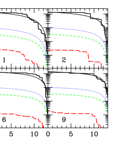
Figure 1.— The mass assembly histories for halos 1, 2, 6, and 9. Solid jagged lines show the histories for the dark matter halos, $M_{\rm vir}(<t)$, generated via the EPS merger tree method. Smooth solid lines show our best-fit “smooth” accretion history used for the background potential in our N-body simulations (Equation 4). Smooth dotted and short-dashed lines show the evolution in our disk and bulge component masses used to set the galactic contributions to the N-body potentials (Equations 8 - 9). The long-dashed lines show our (main) results for stellar halo assembly histories. Stellar mass is assigned to the stellar halo component at the time it becomes unbound from an accreted satellite halo. Note that the stellar halo in realization 6 is relatively small compared to the other systems whose dark matter halos are all the same size. This is because dark matter halo 6 accumulated most of its mass relatively early, when the stellar mass fractions of accreted satellites were small. Note also that halo 9 has experienced a very recent, massive disruption accretion event, which causes its stellar halo mass to increase sharply at a recent lookback time. This event is seen clearly in the image of halo 9 shown in Figure 14.

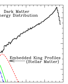
Figure 2.— The energy distribution function of our initial condition dark matter halo (histogram, $dM/d\epsilon$) along with three example energy distributions for stellar matter, $(dM/d\epsilon)_{\star}$, in satellites. The mass to light ratio of each particle of energy $\epsilon$ is assigned based on the ratio of $(dM/d\epsilon)_{\star}$ to $(dM/d\epsilon)$. Energy in this plot is in units of $GM_{35}^{2}/2R_{\rm halo}$.

Figure 3.— V-band luminosity plotted against the ratio of mass in HI to V-band luminosity for satellites of the Milky Way and Andromeda (open symbols) and field dwarfs (solid symbols). Data is taken from the compilation by Grebel, Gallagher, & Harbeck (2003)

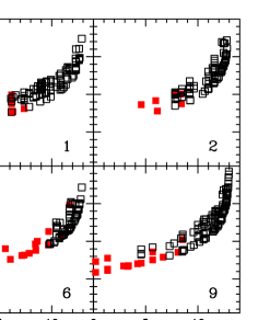
Figure 4.— Plotted is the gas mass per stellar luminosity ratio $M_{\rm gas}/L_{\rm V}$ for each accreted satellite at the time of their accretion, $t_{\rm accr}$, for four example halos. Early accreted systems are more gas rich owing to the rather long star formation timescales in these systems. Solid points points indicate satellites that survive until the present day.

Figure 5.— Histograms of the distribution of Milky Way satellites (solid lines) and simulated satellites (dashed lines — from all 11 halos) as functions of observed quantities

Figure 6.— Derived KS statistic for the satellite distribution in each simulated halo compared with those from the combined sample (solid line) and the observed Milky Way distribution (dotted line).

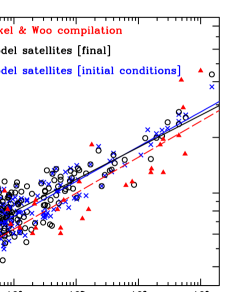
Figure 7.— The relationship between the central, 1-D stellar velocity dispersion and satellite mass for all of our surviving model satellites. Crosses show surviving satellites at the current epoch and open circles show the relationship computed before the satellites were accreted into the host dark matter halo. Solid triangles show the same relationship for local group satellites as compiled by Dekel & Woo (2003). The two nearly identical solid lines show the best-fit regressions for the initial and final model populations. The dashed line shows the best-fit line for the data. The best-fit lines all have similar slopes, $\sigma_{*}\propto M_{*}^{a}$ with $a\simeq 0.2$ ($a=0.19,0.18$ and $0.19$ for initial, final, and data populations respectively, and with errors of $0.01$ in $a$ and $\sim 0.07$ in logarithmic normalization.). The model satellites match the observed trend in the data quite well, considering the observational uncertainties (see, e.g. the discussion in Dekel & Woo, 2003).

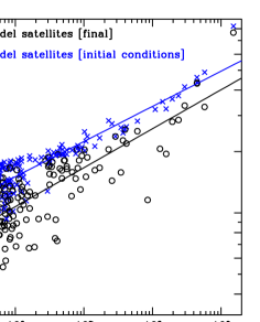
Figure 8.— The the central, 1-D velocity dispersion in the dark matter versus satellite stellar mass. As in Figure 7, crosses show surviving model satellites and open circles show the relationship computed before those systems were accreted into the host dark matter halo. The lines again show least square regression fits, $\sigma_{\rm DM}\propto M_{*}^{b}$. The final systems tend to have lower velocity dispersions and a broader scatter at fixed stellar mass owing to the loss of loosely-bound dark matter particles after accretion. Compare this result to Figure 7, where very little shift occurs in the more tightly bound stellar material.

Figure 9.— Density profiles for our four example simulated stellar halos (thin solid lines). compared to the dark matter halo (bold lines). Dotted lines represent a power law with exponent -3.

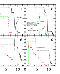
Figure 10.— The cumulative fraction of stellar halo mass built from accreted satellite galaxies as a function of the accretion time of the satellites for halos 1-4. Solid lines show the full halo and dotted lines show the contribution from satellite halos more massive than $M_{\rm vir}>2\times 10^{10}M_{\odot}$ at the time of their accretion. While for halos (1,2,6, and 9) only (18,10,12,13) of the (115,102, 182, 153) accreted luminous satellites were more massive than $2\times 10^{10}M_{\odot}$, we see that $\sim 75-90\%$ of the mass associated with each stellar halo originated within massive satellites of this type. For comparison, the dashed lines show the cumulative fraction of surviving satellite galaxies as a function of the time they were accreted. Short-dashed lines also show the cumulative accretion times of surviving satellites, except now restricted to satellite halos that were more massive than $M_{\rm vir}\lower 2.58334pt\vbox{\hbox{$\buildrel\textstyle>\over{\sim}\ $}}5\times 10^{9}M_{\odot}$ at the time of their accretion We see that surviving halos tend to be accreted later than destroyed halos. There is also a tendency for massive satellites that survive to be accreted even later because the destructive effects of dynamical friction are more important for massive satellites.

Figure 11.— Top panel compares the luminosity fraction of the entire stellar halo spherical shells at radius $r$ from the center of the parent galaxy (solid lines) with the contribution from events since the last $>$ 10% merger event (dotted lines). Bottom panel compares the number fraction of Milky Way satellites in spherical shells as a function of Galactocentric distance (solid line) with the number fraction of our surviving satellite population taken from all eleven simulated halos (dashed line).

Figure 12.— The number fraction of all events, binned in satellite lunminosity, contributing to all eleven of our simulated halos (dotted lines) compared to the number fraction of surviving satellites (dashed lines). The solid lines show the fraction of the total luminosity contributed by each range of satellite luminosities.

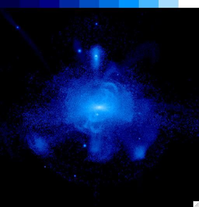
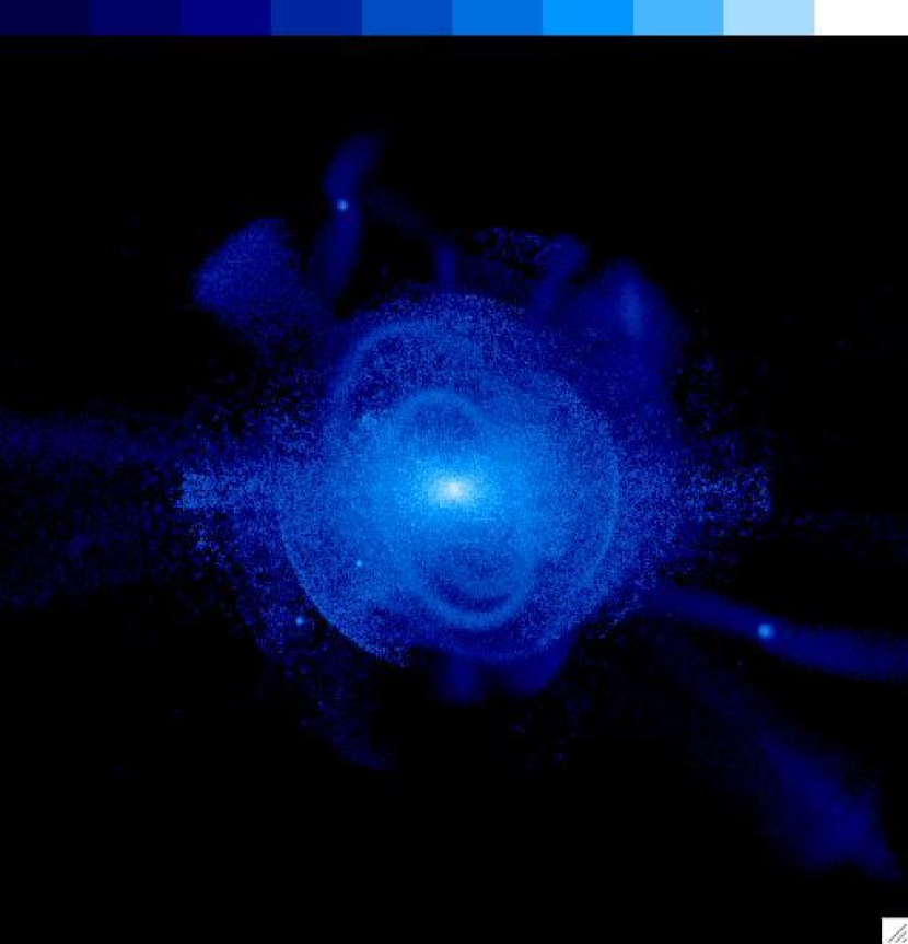
Figure 13.— “External Galaxy” views for halo realizations 1 (left) and 2 (right). The boxes are 300 kpc by 300 kpc. The blue/white color scale indicates surface brightness: 23 Magnitudes per square arcsecond (white) to 38 Magnitudes per square arcsecond (dark blue / black) where we have assumed a stellar mass to light ratio of 2. The eye picks up lighter blue (middle of the bar) at about 30 Magnitudes per square arcsecond.

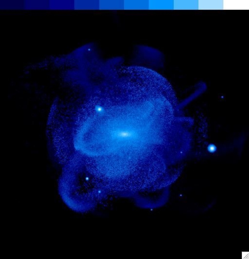
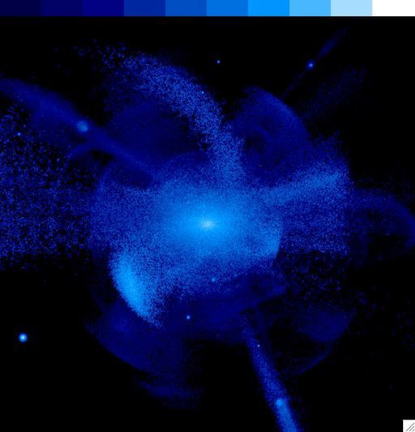
Figure 14.— “External Galaxy” images for halos 6 (left) and 9 (right). The color codes are the same as those in Figure 13. A recent disruption has occurred in halo 9 ($\sim 1.5$Gyr lookback time) and the residue of this event is seen as the bright plume running from the “north-west” of the halo (upper left) down towards the halo center. The bright feature just to the “south-west” of halo 9’s center is also associated with the same disruption event.

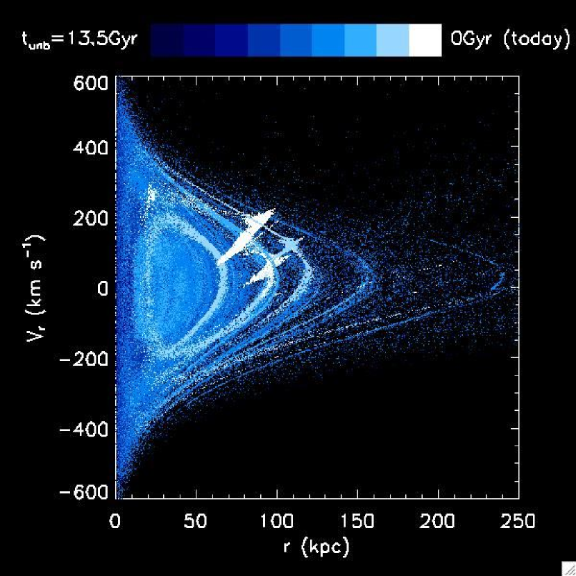
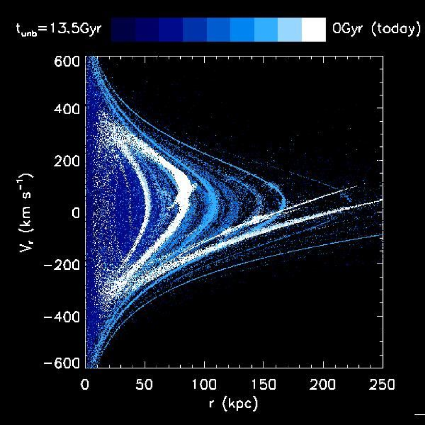
Figure 15.— Radial phase space diagrams ($V_{r}$ vs $r$ relative to the host halo center) for halos 1 (left) and 9 (right). Each point represents 1000 solar luminosities. The color code reflects the time each particle became unbound to its parent satellite. White points are either bound or became unbound in the last 1.5 Gyr, while dark blue points became unbound more than 12 Gyr ago. The radial color gradient reflects the tendency for inner halo stars to be accreted (and stripped) early in the Galaxy’s history. The white feature at $r\sim 80$ kpc in halo 9 represents a very recent disruption event – the most recent massive disruption seen in our ensemble of 11 halo realizations.

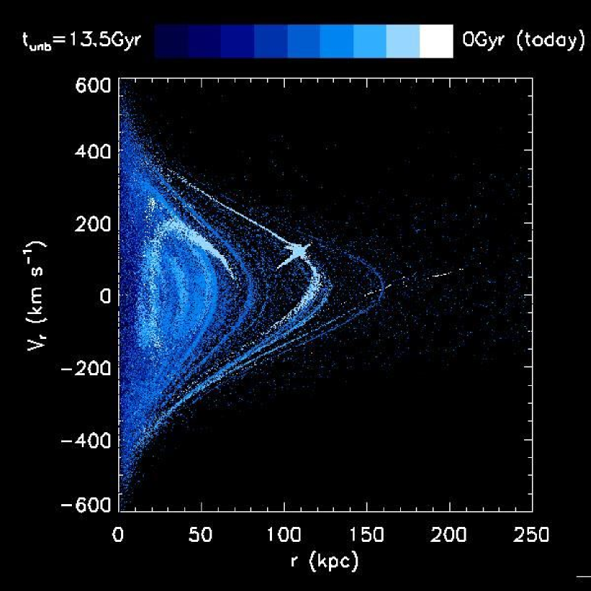
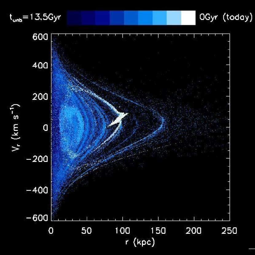
Figure 16.— Radial phase space diagrams for halo 2, where the left and right figures represent to separate quarters of the sky. The color code and axis labels are the same as those in Figure 15.

References

- Abadi et al. (2003) Abadi, M. G., Navarro, J. F., Steinmetz, M., & Eke, V. R. 2003, ApJ, 597, 21
- Barkana & Loeb (1999) Barkana, R., & Loeb, A. 1999, ApJ, 523, 54
- Benson et al. (2002) Benson, A. J., Lacey, C. G., Baugh, C. M., Cole, S., & Frenk, C. S. 2002, MNRAS, 333, 156
- Benson (2005) Benson, A. J. 2005, MNRAS, 358, 551
- Binney & Tremaine (1987) Binney, J. & Tremaine, S. 1987, ”Galactic Dynamics”, Princeton University Press, 1987, 747 p.,
- Blitz & Robishaw (2000) Blitz, L., & Robishaw, T. 2000, ApJ, 541, 675
- Blumenthal et al. (1984) Blumenthal, G. R., Faber, S. M., Primack, J. R., & Rees, M. J. 1984, Nature, 311, 517
- Bryan & Norman (1998) Bryan, G. L., & Norman, M. L. 1998, ApJ, 495, 80
- Bullock, Kravtsov, & Weinberg (2000) Bullock, J.S., Kravtsov, A.K., Weinberg, D.H., 2000, ApJ, 539, 517
- Bullock et al. (2001) Bullock, J. S., Kolatt, T. S., Sigad, Y., Somerville, R. S., Kravtsov, A. V., Klypin, A. A., Primack, J. R., & Dekel, A. 2001, MNRAS, 321, 559
- Bullock, Kravtsov, & Weinberg (2001) Bullock, J. S., Kravtsov, A. V., & Weinberg, D. H. 2001, ApJ, 548, 33
- Bullock & Johnston, (2005) Bullock, J.S. & Johnston, K. V. 2005, in prep
- Brook et al. (2003) Brook, C. B., Kawata, D., Gibson, B. K., & Flynn, C. 2003, ApJ, 585, L125
- Brook et al. (2004b) Brook, C. B., Kawata, D., Gibson, B. K., & Flynn, C. 2004, MNRAS, 349, 52
- Brook et al. (2004a) Brook, C. B., Kawata, D., Gibson, B. K., & Freeman, K. C. 2004, ApJ, 612, 894
- Brook et al. (2005a) Brook, C. B., Gibson, B. K., Martel, H., & Kawata, D. 2005a, ArXiv Astrophysics e-prints, arXiv:astro-ph/0503273
- Brook et al. (2005b) Brook, C. B., Martel, H., Gibson, B. K., & Kawata, D. 2005b, ArXiv Astrophysics e-prints, arXiv:astro-ph/0503323
- Chiba & Beers (2000) Chiba, M. & Beers, T. C. 2000, AJ, 119, 2843
- Chiu et al. (2001) Chiu, W. A., Gnedin, N. Y., & Ostriker, J. P. 2001, ApJ, 563, 21
- Dekel & Woo (2003) Dekel, A., & Woo, J. 2003, MNRAS, 344, 1131
- D’Onghia & Burkert (2004) D’Onghia, E., & Burkert, A. 2004, ApJ, 612, L13
- Crane et al. (2003) Crane, J. D., Majewski, S. R., Rocha-Pinto, H. J., Frinchaboy, P. M., Skrutskie, M. F., & Law, D. R. 2003, ApJ, 594, L119
- Eggen, Lynden-Bell, & Sandage (1962) Eggen, O. J., Lynden-Bell, D., & Sandage, A. R. 1962, ApJ, 136, 748