Direct detection of the inflationary gravitational wave background

Abstract

Inflation generically predicts a stochastic background of gravitational waves over a broad range of frequencies, from those accessible with cosmic microwave background (CMB) measurements, to those accessible directly with gravitational-wave detectors, like NASA’s Big-Bang Observer (BBO) or Japan’s Deci-Hertz Interferometer Gravitational-wave Observer (DECIGO), both currently under study. Here we investigate the detectability of the inflationary gravitational-wave background at BBO/DECIGO frequencies. To do so, we survey a range of slow-roll inflationary models consistent with constraints from the CMB and large-scale structure (LSS). We go beyond the usual assumption of power-law power spectra, which may break down given the 16 orders of magnitude in frequency between the CMB and direct detection, and solve instead the inflationary dynamics for four classes of inflaton potentials. Direct detection is possible in a variety of inflationary models, although probably not in any in which the gravitational-wave signal does not appear in the CMB polarization. However, direct detection by BBO/DECIGO can help discriminate between inflationary models that have the same slow-roll parameters at CMB/LSS scales.

I Introduction

Long a subject of theoretical speculation, inflation Guth (1981); Albrecht and Steinhardt (1982); Linde (1982a) has now, with the advent of precise cosmic microwave background (CMB) measurements Kamionkowski and Kosowsky (1999); de Bernardis et al. (2000); Miller et al. (1999); Hanany et al. (2000); Halverson et al. (2002); Mason et al. (2003); Benoit et al. (2003); Goldstein et al. (2003); Spergel et al. (2003), become an empirical science. The concordance of the measurements with the inflationary predictions of a flat Universe and a nearly scale-invariant spectrum of primordial density perturbations Guth and Pi (1982); Bardeen et al. (1983); Hawking (1982); Linde (1982b) is at least suggestive and warrants further tests of inflation. Among the predictions of inflation yet to be tested is a stochastic gravitational-wave background with a nearly scale-invariant spectrum Starobinsky (1979); Abbott and Wise (1984); Starobinskii (1985); Rubakov et al. (1982); Fabbri and Pollock (1983); Allen (1988); Sahni (1990). Detection of the CMB polarization pattern induced by inflationary gravitational waves of wavelengths comparable to the horizon has become a goal of next-generation CMB experiments Kamionkowski et al. (1997a, b); Zaldarriaga and Seljak (1997); Seljak and Zaldarriaga (1997); Cabella and Kamionkowski (2004). And now, direct detection of the inflationary gravitational wave background (IGWB) with future spaced-based gravitational-wave detectors at deci-Hertz frequencies has become the subject of serious study BBO ; Seto et al. (2001).

Detection of a gravitational-wave background, at either CMB or direct-detection frequencies, would constitute a “smoking gun” for inflation. Moreover, since the amplitude of the IGWB is determined by the energy scale of inflation at the time that the relevant distance scale exited the horizon during inflation, detection would provide important information about the new ultra-high-energy physics responsible for inflation Kamionkowski and Kosowsky (1998); Jaffe et al. (2000). Since the frequencies probed by the CMB and by direct detection are separated by 16 orders of magnitude, the combination of both provides a large lever arm with which the shape of the inflaton potential can be constrained.

In this paper, we survey a range of inflationary models to investigate the detectability of the IGWB with satellite experiments, like NASA’s Big Bang Observer (BBO) BBO and the Japanese Deci-Hertz Interferometer Gravitational-wave Observatory (DECIGO) Seto et al. (2001), currently under study. We restrict our attention to slow-roll inflation models that are consistent with measurements from the CMB and large-scale structure. We show how measurements of the IGWB amplitude at both CMB and direct-detection scales can be used to constrain the inflationary parameter space.

Previous work Bar-Kana (1994); Turner (1997); Ungarelli et al. (2005) on direct detection of the IGWB has taken the gravitational-wave spectrum to be a pure power law, considered chaotic inflation Liddle (1994); Battye and Shellard (1996) or the IGWB due to a broken scale invariant potential Polarski (1999). In this paper, we consider a wider range of inflationary models (in the spirit of Refs. Dodelson et al. (1997); Kinney (1998)), and we solve the inflationary dynamics to go beyond the assumption of power-law power spectra. With this more accurate analysis, we find that for the forms of the inflaton potential considered here the direct detection of the IGWB can break degeneracies between distinct inflationary models that produce the same slow-roll parameters at CMB/large-scale-structure scales for broken scale invariant potentials.

This paper is organized as follows. In Section II, we review the basics and relevant ingredients of inflation as well as constraints from the CMB and large-scale structure (LSS) to the inflationary observables. We also discuss the transfer function that relates the current gravitational-wave amplitude to its primordial value. In Section III, we discuss the sensitivities of planned space-based gravitational-wave observatories to the IGWB. In Section IV, we show for four different families of slow-roll inflation models the IGWB amplitude and spectral index $n_{t}$ at BBO/DECIGO scales that are allowed by current CMB/LSS constraints to the $n_{s}$–$r$ parameter space (where $n_{s}$ is the scalar spectral index and $r$ the tensor-to-scalar ratio). Section V compares the results of our calculations with those obtained by extrapolating the power-law power spectra inferred from CMB/LSS measurements to BBO/DECIGO scales. In section VI we discuss a family of slow-roll inflation models where the observational signature in CMB/LSS studies for two different models is the same but differs for the direct detection of the IGWB at BBO/DECIGO scales. In Section VII, we summarize and make some concluding remarks.

II Inflationary Dynamics and Perturbations

II.1 Homogeneous Evolution

Inflation occurs when the cosmological expansion accelerates; i.e., when $\ddot{a}>0$, where $a(t)$ is the scale factor, and the overdot denotes a derivative with respect to time $t$. The evolution of the scale factor is determined by the Friedmann equation,

$$H^{2}\equiv\left(\frac{\dot{a}}{a}\right)^{2}=\frac{8\pi}{3M_{\mathrm{Pl}}^{2}}\rho-\frac{K}{a^{2}},$$ (1)

the continuity equation, $\dot{\rho}+3H(\rho+P)=0$, and an equation of state $P(\rho)$, where $H$ is the Hubble parameter, $\rho$ is the total energy density, $P$ is the pressure, $M_{\mathrm{Pl}}$ is the Planck mass, and $K$ is a constant related to the 3-space curvature. From Eq. (1) and the continuity equation follows the “acceleration” equation,

$$\frac{\ddot{a}}{a}=-\frac{4\pi}{3M_{\mathrm{Pl}}^{2}}(\rho+3P).$$ (2)

For an equation of state of the form $P=w\rho$, where $w$ is a constant, inflation occurs when $w<-1/3$.

Consider now a spatially homogeneous scalar field $\phi$, the “inflaton”. It has an energy density and pressure,

$$\rho = \frac{1}{2}\dot{\phi}^{2}+V(\phi),$$ (3)

$$P = \frac{1}{2}\dot{\phi}^{2}-V(\phi),$$ (4)

from which it follows that inflation occurs if $V(\phi)>\dot{\phi}^{2}$.

The equation of motion for the inflaton is given by $\ddot{\phi}+3H\dot{\phi}+V^{\prime}=0$, where the prime denotes differentiation with respect to $\phi$. We assume that inflation has been proceeding for a long time before any observable scales have exited the horizon, and so for our purposes, the energy density is dominated by the inflaton during inflation, the curvature term, $K/a^{2}$, is negligible as compared to the inflaton energy density, and the evolution of the inflaton has been attracted to the slow-roll regime (e.g., Ref. Liddle et al. (1994)). If so, the evolution of the inflaton and the scale factor are uniquely determined by $V(\phi)$. Within the slow-roll approximation, the evolution is described by the usual slow-roll parameters,

$$\epsilon \equiv \frac{M_{\mathrm{Pl}}^{2}}{16\pi}\left(\frac{V^{\prime}}{V}\right)^{2},$$ (5)

$$\eta \equiv \frac{M_{\mathrm{Pl}}^{2}}{8\pi}\frac{V^{\prime\prime}}{V},$$ (6)

$$\xi \equiv \frac{M_{\mathrm{Pl}}^{4}}{64\pi^{2}}\frac{V^{\prime}V^{\prime\prime\prime}}{V^{2}},$$ (7)

which are required to be small compared with unity for the slow-roll approximation to be valid. Toward the end of inflation, $\epsilon$ grows, and inflation ends when $\epsilon\simeq 1$. This statement can be made precise by the use of “Hubble slow-roll” parameters Liddle et al. (1994).

II.2 Perturbations

To leading order in the slow-roll approximation, the amplitudes of the power spectra for density perturbations (scalar “s” metric perturbations) and gravitational waves (tensor “t” metric perturbations) can be written (e.g., Refs. Stewart and Lyth (1993a); Lidsey et al. (1997))

$$P_{s}(k) \approx \frac{128\pi}{3M_{\mathrm{Pl}}^{6}}\frac{V^{3}}{V^{\prime 2}}\Bigg{|}_{k=aH},$$ (8)

$$P_{t}(k) \approx \frac{128}{3}\frac{V}{M_{\mathrm{Pl}}^{4}}\Bigg{|}_{k=aH},$$ (9)

as a function of wavenumber $k$, where $V$ and $V^{\prime}$ are evaluated when the relevant scale exits the horizon during inflation. The power spectra can be expanded in power laws,

$$P_{s}(k) \approx P_{s}(k_{0})\left(\frac{k}{k_{0}}\right)^{1-n_{s}+(\alpha_{s}/2)\ln(k/k_{0})},$$ (10)

$$P_{t}(k) \approx P_{t}(k_{0})\left(\frac{k}{k_{0}}\right)^{n_{t}+(\alpha_{t}/2)\ln(k/k_{0})},$$ (11)

where $k_{0}$ is a pivot wavenumber at which the spectral parameters (e.g., Ref. Liddle and Lyth (2000)),

$$n_{s}(k) \simeq 1-6\epsilon+2\eta,$$ (12)

$$n_{t}(k) \simeq -2\epsilon,$$ (13)

$$\alpha_{s}(k) \simeq 16\epsilon\eta-24\epsilon^{2}-2\xi,$$ (14)

$$\alpha_{t}(k) \simeq 4\epsilon\eta-8\epsilon^{2},$$ (15)

are to be evaluated. To a first approximation, the power spectra are power laws with power-law indices $n_{s}$ and $n_{t}$, although these indices may “run”slightly with $k$, with a running parameterized by $\alpha_{s}$ and $\alpha_{t}$ Kosowsky and Turner (1995). Finally, the tensor-to-scalar ratio is

$$r\equiv\frac{P_{t}(k)}{P_{s}(k)}=16\epsilon.$$ (16)

In this paper, we will generally evaluate $P_{s}$, $n_{s}$, and $\alpha_{s}$ at the distance scales of the CMB and large-scale structure (LSS), where they are measured or constrained. In the Figures below, the tensor spectral index $n_{t}$ will be evaluated at the distance scale relevant for direct detection of gravitational waves.

II.3 Number of $e$-Foldings

The number of $e$-foldings of expansion between the time, determined by $k=a_{k}H_{k}$, when a comoving distance scale labeled by $k$ exited the horizon during inflation, and the end of inflation is $N(k)\equiv\ln\left(a_{\mathrm{end}}/a_{k}\right)$, where $a_{\mathrm{end}}$ is the scale factor at the end of inflation. This must be (e.g., Ref. Liddle and Lyth (1993)),

$$N(k)=$$ (17)

$$62-\ln\frac{k}{a_{0}H_{0}}-\ln\frac{10^{16}\ \mathrm{GeV}}{V_{k}^{1/4}}+\ln\frac{V_{k}^{1/4}}{V_{\mathrm{end}}^{1/4}}-\frac{1}{3}\ln\frac{V_{\mathrm{end}}^{1/4}}{\rho_{\mathrm{rh}}^{1/4}},$$

where $V_{k}$ is the inflaton potential when the comoving scale $k$ crossed the inflationary horizon; $V_{\mathrm{end}}$ is the value of the potential at the end of inflation; and $\rho_{\mathrm{rh}}\sim T_{\mathrm{rh}}^{4}$ is the energy density of the universe once radiation domination begins. Here we have assumed that the Universe was matter dominated after inflation and before reheating and that the transition between radiation and matter domination is instantaneous. In terms of the inflaton potential, the number of $e$-foldings between two field values, $\phi_{i}$ and $\phi_{f}$, is

$$N(\phi_{i},\phi_{f})\approx\frac{8\pi}{M_{\mathrm{Pl}}^{2}}\int_{\phi_{f}}^{\phi_{i}}\frac{V(\phi)}{V^{\prime}(\phi)}d\phi,$$ (18)

where we have supposed the potential increases as the field increases so that the field rolls towards the origin. Furthermore, if the potential determines a field value at which inflation ends, we can combine this equation with Eq. (17) and $\rho_{\mathrm{rh}}$ to identify the field value when the current Hubble volume exited the inflationary horizon.

If we use $10^{16}$ GeV for all the densities in Eq. (17), we require 62 $e$-folds of inflation between the time the current horizon distance exited the horizon during inflation and the end of inflation. The strength of the IGWB is proportional to the inflaton-potential height [cf., Eq. (9)], and as we will see, detectability requires $V\gtrsim 10^{15}$ GeV. We will also see that $V_{\mathrm{end}}$ is never much smaller than $V_{k}$. Thus, the only ratio in Eq. (17) that might be large is the last. Conservatively, the reheat temperature must be $\gtrsim$ 1 MeV to preserve the successes of big-bang nucleosynthesis, implying a lower limit of $N(a_{0}H_{0})\gtrsim 47$. This lower limit is significant, as the ratio of gravitational-wave frequencies probed by the CMB/LSS (corresponding to $k\simeq 0.05\,\mathrm{Mpc}^{-1}$) and direct detection is $\sim e^{35}$. Therefore, if inflation results in an IGWB in the ballpark of detectability by the CMB, then inflation will last long enough to ensure the production of gravitational waves on BBO/DECIGO scales (although it does not necessarily guarantee a detectable amplitude).

II.4 Constraints to Inflationary Observables

We would like to survey only those inflationary models that are consistent with current data. Measurements of the “inflationary observables”—i.e., the scalar and tensor power-spectrum amplitudes, spectral indices, and running—come from CMB measurements that probe scales from the current Hubble distance ($\sim 10^{4}$ Mpc) to $\sim 10$ Mpc scales, galaxy surveys that constrain the matter power spectrum from $600\ \mathrm{Mpc}$ down to $20\ \mathrm{Mpc}$, and from the Lyman-$\alpha$ forest, which probes down to $\sim$ 1 Mpc Croft et al. (1998); Mandelbaum et al. (2003). Constraints to the classical cosmological parameters (e.g., the Hubble parameter, the deceleration parameter, the baryon density, the matter density) from other measurements help limit the range of plausible values for the inflationary observables that come from CMB/LSS measurements.

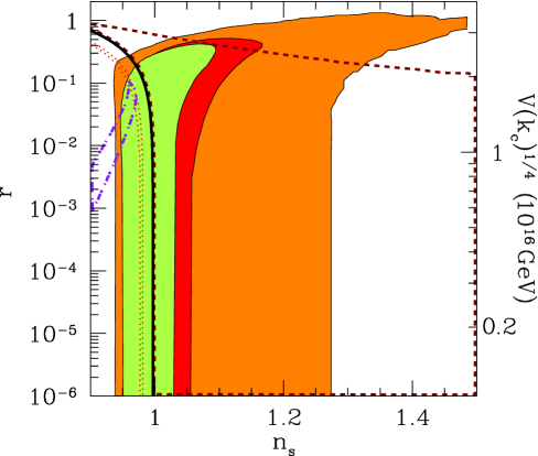
Figure 1: Regions in the $n_{s}$–$r$ parameter space consistent with the CMB-only (orange/medium gray) Peiris et al. (2003), CMB plus galaxy surveys (red/dark gray), and CMB plus galaxy surveys plus Lyman-alpha-forest constraints (green/light gray) Seljak et al. (2004). Here, $r$ is the tensor-to-scalar ratio, and $n_{s}$ is the scalar spectral index at CMB scales. We plot on top of these regions the parameter space occupied by the four models of inflation we consider: power-law (solid black line), chaotic (dotted red), symmetry-breaking (dashed-dot purple) and hybrid (short-dashed dark-red). The right axis shows the energy scale $[V(k_{c})]^{1/4}$ of inflaton.

The precise constraints to the inflationary observables depend in detail on the combination of observational data sets. In our discussions, we simply take as conservative ranges $P_{s}(k_{0})=(2.45\pm 0.23)\times 10^{-9}$, $n_{s}=1.0\pm 0.1$, and $|\alpha_{s}|<0.04$ at a pivot wavenumber $k_{0}=0.05\ \mathrm{Mpc}^{-1}$ Seljak et al. (2004). We note that the CMB-only constraints correspond to a pivot wavenumber, $k_{0}=0.002\ \mathrm{Mpc}^{-1}$ Peiris et al. (2003). The errors we quote are not to be interpreted as statistical errors bars, except in the case of the value for $P_{s}(k_{0})$, where the error quoted is $1\sigma$; rather, they simply indicate a range of parameters that are in reasonable concordance with measurements Bennett et al. (2003); Peiris et al. (2003); Tegmark et al. (2004); Seljak et al. (2004) and the range of values that we use here. In our discussion, we take a conservative upper limit $r\lesssim 1$ to the tensor-to-scalar ratio. The numerical results we show in Fig. 3 use slow-roll parameters consistent with the regions in the $n_{s}$–$r$ parameter space, shown in Fig. 1, taken from analyses of CMB data alone, CMB plus galaxy surveys, and CMB, galaxies, and the Lyman-alpha forest Peiris et al. (2003); Seljak et al. (2004).

II.5 Gravitational-Wave Transfer Function

The gravitational-wave power spectrum $P_{t}(k)$ provides the variance $\langle|h_{k}|^{2}\rangle$ of the gravitational-wave amplitude $h_{k}$ as that mode enters the horizon. Once the wavelength is smaller than the horizon, the gravitational wave begins to oscillate, and its energy density $\rho_{k}\sim k^{2}h_{k}^{2}$ redshifts $\propto a^{-4}$ like radiation. It follows that the gravitational-wave amplitude today is $h_{k}(t_{0})=h_{k}(t_{k})(a_{k}/a_{0})$, where $t_{0}$ is the time today, $t_{k}$ is the time of horizon entry, and $a_{k}=a(t_{k})$ . During radiation domination (RD), $H\propto a^{-2}$, so that $k\propto 1/a_{k}$, and during matter domination (MD), $H\propto a^{-3/2}$, so that $k\propto 1/a_{k}^{1/2}$. From these relations, we find that the value of $h_{k}$ today scales with $k$ as

$$h_{k} \propto k^{-1}\ \mathrm{(horizon\ entry\ during\ RD)},$$ (19)

$$h_{k} \propto k^{-2}\ \mathrm{(horizon\ entry\ during\ MD)}.$$ (20)

Calculations (e.g., Refs. Turner et al. (1993); Pritchard and Kamionkowski (2004)) of the transfer function intended for CMB predictions evolve the wave equation more carefully through matter-radiation equality, but the direct-detection frequencies are so high that the scalings we have used here are fairly precise. The sensitivities of BBO/DECIGO will peak near a frequency 0.1 Hz, or wavenumber $k=6.47\times 10^{13}\,\mathrm{Mpc}^{-1}$. Matter-radiation equality corresponds to $k_{\mathrm{eq}}\approx 0.05h^{2}\,\mathrm{Mpc}^{-1}$. Therefore, the primordial gravitational waves observed by the planned gravitational-wave observatories entered the horizon well before matter/radiation equality. In fact, the modes that entered the horizon during big-bang nucleosynthesis (at $T\sim 1$ MeV) have frequencies $\sim 10^{-11}$ Hz. Therefore, the gravitational waves probed by BBO/DECIGO are $\sim 10$ orders of magnitude smaller than those associated with big-bang nucleosynthesis (BBN) and must have entered the horizon at temperatures $T\sim 10^{7}$ GeV.

These high temperatures imply a small correction to previous calculations, which assumed $T\propto a^{-1}$, of the transfer function due to the fact that it is actually $g_{*S}(T)a^{3}T^{3}$ that remains constant, where $g_{*S}(T)$ is the effective number of relativistic degrees of freedom contributing to the entropy density. Recalling that the Hubble parameter is $H\simeq 1.66\,g_{*}^{1/2}T^{2}/M_{\mathrm{Pl}}$ during radiation domination (where $g_{*}$ is the effective number of relativistic degrees of freedom contributing to the energy density; at these temperatures, $g_{*}\simeq g_{*S}$), the condition for horizon entry for a physical wavenumber today ($a_{0}k=a_{k}H_{k}$), becomes

$$1.66\,g_{*}^{1/2}(T_{k})(T_{0}T_{k}/M_{\mathrm{Pl}})\left(\frac{g_{*S}(T_{0})}{g_{*S}(T_{k})}\right)^{1/3}=k.$$ (21)

Today, $g_{*S}(T_{0})=3.91$ for photons and three species of massless neutrinos. We then have,

$$\left(\frac{T_{k}}{3.8\times 10^{6}\,\mathrm{GeV}}\right)\left[\frac{g_{*}(T_{k})}{100}\right]^{1/6}=\left(\frac{k}{6.5\times 10^{13}\,\mathrm{Mpc}^{-1}}\right).$$ (22)

Taking only standard-model particles, $g_{*}(T)\approx 100$ (or roughly double if there is low-energy supersymmetry) and should be roughly independent of temperature. We thus find that for BBO/DECIGO scales,

$${\cal T}(k)=\frac{a_{k}}{a_{0}}=2.1\times 10^{-20}\left(\frac{k}{6.5\times 10^{13}\mathrm{Mpc}^{-1}}\right)^{-1}g_{100}^{-1/6},\\$$ (23)

where $g_{100}\equiv g_{*}(T_{k})/100$. With this transfer function, the root-variance of the IGWB today is

$$\langle|h_{k}|^{2}\rangle^{1/2}=P_{t}(k)^{1/2}\mathcal{T}(k).$$ (24)

Free streaming of neutrinos, which occurs after neutrinos decouple at a temperature $\sim 1\ \mathrm{MeV}$, contributes an anisotropic stress Weinberg (2004); Bashinsky (2005). However, the resulting damping will be negligible for modes that enter the horizon so much earlier than neutrino free-streaming.

If we define the logarithmic GW contribution to the critical density,

$$\Omega_{\mathrm{GW}}(k)\equiv\frac{1}{\rho_{c}}\frac{d\rho_{\mathrm{GW}}}{d\ln k},$$ (25)

then Maggiore (2000),

$$\Omega_{\mathrm{GW}}(k)h^{2}=\frac{c^{2}k^{2}h^{2}}{6H_{0}^{2}}\langle|h_{k}|^{2}\rangle\equiv A_{\mathrm{GW}}P_{t}(k),$$ (26)

where $H_{0}\equiv 100\,h\ \mathrm{km}\,\mathrm{s}^{-1}\,\mathrm{Mpc}^{-1}$, and $A_{\mathrm{GW}}=2.74\times 10^{-6}\,g_{100}^{-1/3}$. In slow-roll inflation, $n_{t}<0$, so if we take $P_{s}(k_{0})\simeq 2.45\times 10^{-9}$ and $r\lesssim 1$ (corresponding to $V^{1/4}\lesssim 3.36\times 10^{16}$ GeV), we find an upper limit $\Omega_{\mathrm{GW}}h^{2}\lesssim 6.71\times 10^{-15}g_{100}^{-1/3}$.

III Direct-Detection Thresholds

Since the detection of a stochastic background of gravitational waves has to be separated from the effect of sources of noise intrinsic to the detector, the sensitivity to a stochastic background is different than the sensitivity to a non-stochastic source. The total stochastic signal in a given detector can be written as a sum of a stochastic signal plus a stochastic noise, $s(t)=h_{n}(t)+h(t)$. Taking the Fourier transform of the total signal and considering the spectral density of the noise and of the stochastic signal, we find that in order to have a signal-to-noise greater than unity,

$$\left\langle|h(f)|^{2}\right\rangle^{1/2}\gtrsim\left(\frac{2fS_{n}(f)}{F}\right)^{1/2},$$ (27)

where $F$ is a filling factor that accounts for the fact that a primordial stochastic background will be isotropic on the sky, but the detector will only be sensitive to a fraction of the sky, while $S_{n}(f)$ is the spectral density associated with the detector noise.

For omni-directional interferometers, such as the Laser Interferometer Space Antenna (LISA), $F=2/5$. There is a great improvement in sensitivity when the signal from two independent detectors can be combined through a correlation analysis between the two detectors Christensen (1992); Flanagan (1993); Maggiore (2000); Cornish and Larson (2001). Such a correlation increases the sensitivity to a stochastic background such that,

$$\left\langle|h(f)|^{2}\right\rangle^{1/2}\gtrsim$$ (28)

$$1.12\times 10^{-2}\left(\frac{2fS_{n}(f)}{F}\right)^{1/2}\left(\frac{\mathrm{Hz}}{\Delta f}\right)^{1/4}\left(\frac{\mathrm{yr}}{\Delta T}\right)^{1/4},$$

where $\Delta f$ is the bandwidth over which the signals can be correlated and $\Delta T$ is the integration time. For a correlation analysis, the increase in sensitivity is under the assumption that the detector noises are independent between the two detectors, while the only correlation expected is due to stochastic signals such as inflation. For the single detector, the minimum observable strain is independent of the integration time, while for a correlation analysis, long-term observations are essential. While LISA will not allow an opportunity for such a correlation analysis, some mission concept studies for NASA’s Big Bang Observer (BBO) and Japan’s Deci-Hertz Interferometer Gravitational Wave Observatory (DECIGO) consider two (or more) systems such that the improvement related to the correlation analysis can be exploited. The design for LISA currently places the sensitivity at approximately $\Omega_{\mathrm{GW}}h^{2}\sim 10^{-11}$. Current designs for BBO place the sensitivity of a single detector at $\Omega_{\mathrm{GW}}h^{2}\sim 10^{-13}$ and the sensitivity of a correlated extension at $\Omega_{\mathrm{GW}}h^{2}\sim 10^{-17}$. Finally, the ultimate goal for DECIGO is a sensitivity to $\Omega_{\mathrm{GW}}h^{2}\sim 10^{-20}$ Seto et al. (2001), corresponding to $V^{1/4}\sim 1.15\times 10^{15}$ GeV ($r\sim 10^{-6}$).

Besides a sensitivity to a stochastic background, one must also be concerned about sources of a stochastic background, other than inflation. One such source is the background in extragalactic supernovae Buonanno et al. (2004). Such sources have the potential to wash out any signal that would otherwise be observed from a primordial source, but the characterization of the amplitude and frequency dependence of these sources is still uncertain. Other sources of cosmological gravitational-wave backgrounds are white-dwarf/white-dwarf binaries Farmer and Phinney (2003), neutron-star/neutron-star binaries Schneider et al. (2001) and neutron-star/white-dwarf binaries Cooray (2004).

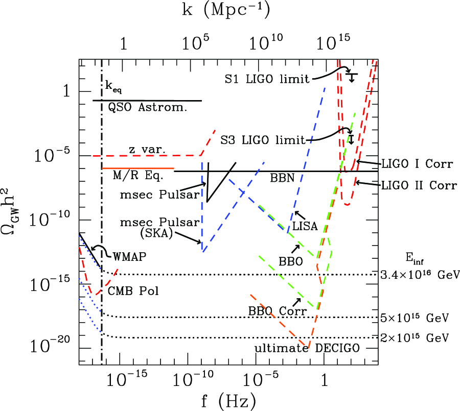
Figure 2: Current limits and projected sensitivities to a stochastic gravitational-wave background versus the gravitational-wave frequency. The solid curves all indicate current upper limits, while the dashed curves indicate projected sensitivities. The LISA curve is from Ref. Larson (2003) and BBO correlated from Ref. Buonanno et al. (2004). The BBO sensitivity is estimated by increasing the BBO-correlated curve by 4 orders of magnitude [see Eq. (III)]. The BBN constraint results from the limit to the number of relativistic degrees of freedom at big-bang nucleosynthesis (e.g., Ref. Allen (1996)); the “M/R” constraint is from CMB/LSS constraints to matter-radiation equality Smith et al. (2005); the “z. var” curve is from Ref. Seto and Cooray (2005); and the quasar-astrometry limit from Refs. Pyne et al. (1996); Gwinn et al. (1997). We note that the BBN and “M/R” constraints assume a scale invariant gravitational-wave background that extends $\sim$ 60 $e$-folds below the current Hubble horizon. LIGO sensitivities, taken from the LIGO Scientific Collaboration White Paper on Detector Research and Development LSC are given in terms of a correlated analysis between the Hanford, WA and Livingston, LA sites [see Eq. (III)]. The run 1 LIGO limit (“S1 LIGO”) is from Ref. Abbott et al. (2004) and the run 3 LIGO limit (“S3 LIGO”) is from Ref. Abbott et al. (2005). Also shown are millisecond-pulsar timing constraints (current Kaspi et al. (1994); Lommen (2002) and sensitivities projected for the Square-Kilometer Array Kramer (2004)). Curves corresponding to scale-invariant (i.e., $n_{t}=0$) gravitational-wave backgrounds are shown (dotted curves), labeled by the associated inflationary energy scales at CMB/LSS scales (but keep in mind that slow-roll inflation generically predicts $n_{t}<0$, less power on small scales). The CMB/LSS currently constrains this value to be below $3.36\times 10^{16}$ GeV at CMB/LSS scales. Future CMB measurements may be able to reach energy scales near $10^{15}$ GeV Kesden et al. (2002); Knox and Song (2002); Seljak and Hirata (2004); Sigurdson and Cooray (2005).

Fig. 2 shows the sensitivities to a stochastic gravitational-wave background as a function of frequency $f$ for a variety of gravitational-wave detectors. Also shown are various current limits (as solid curves) as well as a variety of projected direct and indirect sensitivities (dashed curves), and scale-invariant spectra parameterized by an energy scale $V^{1/4}$ of inflation (dotted curves). We also show limits from current CMB experiments as well as the sensitivities expected for future CMB-polarization experiments currently under study.

IV BBO/DECIGO Amplitudes

In this Section, we calculate the gravitational-wave amplitude at BBO/DECIGO scales for several families of slow-roll inflation models consistent with CMB/LSS constraints.

Measurements of the scalar amplitude $P_{s}$ and spectral index $n_{s}$ at CMB/LSS scales, as well as upper limits to the tensor contribution $r$ to the CMB and to the running $\alpha_{s}$ of the spectral index, constrain the inflaton potential and its derivatives at the field value $\phi_{c}$ that corresponds to the time at which CMB/LSS scales $k_{c}$ exited the horizon. To be precise, we use $k_{c}=0.05\,{\mathrm{Mpc}^{-1}}$. In this work, we take as the nominal BBO/DECIGO frequency $f=0.1$ Hz, corresponding to $k=6.47\times 10^{13}\,{\mathrm{Mpc}^{-1}}$ (and we note that $\Omega_{\rm GW}(k)h^{2}\simeq$ constant for $n_{t}\simeq 0$, so our results will not depend too sensitively on the precise value of $f$ we use). CMB/LSS and BBO/DECIGO scales are therefore separated by $\Delta N=\ln(6\times 10^{13}/0.05)\simeq 35$ $e$-folds of inflation . Eq. (18) can then be used to find the field value $\phi_{g}$ at the time that BBO/DECIGO scales exited the horizon.

IV.1 Power-Law Inflation

In power-law inflation, the inflaton potential takes the form,

$$V(\phi)=V_{0}e^{-p\phi/M_{\mathrm{Pl}}}.$$ (29)

Power-law inflation is so called because the scale factor is a power law $a(t)\propto t^{16\pi/p^{2}}$, and the Hubble parameter also evolves as a power of time $t$. The resulting scalar and tensor power spectra are then pure power laws, with no running of the spectral indices. The parameter $\epsilon=p^{2}/(16\pi)$ always, so that inflation must be ended artificially at some $\phi_{\mathrm{end}}$. Although the potential has only two free parameters ($V_{0}$ and $p$), there is an additional free parameter, namely, the value of $\phi_{\mathrm{c}}$, which we are free to choose in this particular family of models. This model has also $\eta=p^{2}/8\pi$, so $n_{s}=1-p^{2}/8\pi=1-2\epsilon$, and for $n_{s}>0.9$ we find a constraint $\epsilon<0.05$. The constraint $r=16\epsilon\lesssim 1$ is comparable or a bit weaker. Since $n_{s}$ and $r$ depend in this model only on the parameter $p$, these models occupy a curve in the $n_{s}$–$r$ parameters space, which is indicated by the heavy solid curve in Fig. 1. The constraint $\Delta N=35$ to the number of $e$-folds between CMB/LSS and BBO/DECIGO scales tells us that

$$\Delta N=\frac{8\pi}{p}\frac{\phi_{g}-\phi_{c}}{M_{\mathrm{Pl}}}\simeq 35,$$ (30)

from which it follows that

$$\frac{P_{t}(k_{g})}{P_{t}(k_{c})}=\frac{V(\phi_{g})}{V(\phi_{c})}=e^{-(p^{2}/8\pi)\Delta N}=e^{-2\epsilon\Delta N}.$$ (31)

We thus find that the gravitational-wave amplitude at DECIGO/BBO scales is

$$\Omega_{\mathrm{GW}}h^{2} = A_{\rm GW}P_{t}(k_{g})=A_{\rm GW}rP_{s}(k_{c})e^{-2\epsilon\Delta N}$$ (32)

$$= 1.08\times 10^{-13}\epsilon\,e^{-70\,\epsilon(\Delta N/35)}$$

$$\times\left(\frac{P_{s}(k_{c})}{2.45\times 10^{-9}}\right)\left(\frac{A_{\rm GW}}{2.74\times 10^{-6}}\right).$$

This expression is maximized for $\epsilon=1/(2\Delta N)\simeq 1/70$ at a value $\Omega_{\rm GW}^{\rm max}h^{2}=5.68\times 10^{-16}$. Interestingly enough, the IGWB detectability through direct detection is maximized for relatively small $\epsilon$, while the detectability with the CMB is maximized at larger $\epsilon$ Liddle (1994). Given that CMB sensitivities are expected to get to $r\sim 0.01$ in the relatively near future with the CMB, and then to $r\sim 10^{-4}$ with a next-generation satellite experiment, it is unlikely that this model would produce a direct detection without producing a detectable CMB signal.

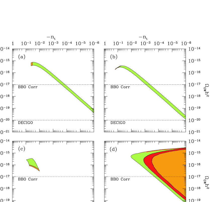
Figure 3: Regions in the $\Omega_{\rm GW}h^{2}$–$n_{t}$ parameter space for (a) power-law, (b) chaotic, (c) symmetry-breaking, and (d) hybrid inflation. The colored (shaded) regions map out the corresponding regions in Fig. 1. Here, the gravitational-wave density $\Omega_{\rm GW}h^{2}$ and spectral index $n_{t}$ are both evaluated at DECIGO/BBO scales. Also shown are the sensitivity goals of BBO and DECIGO.

Fig. 3(a) shows the region of the $\Omega_{\mathrm{GW}}h^{2}$–$n_{t}$ parameter space (at BBO/DECIGO scales) that the $n_{s}$–$r$ parameter space shown in Fig. 1 maps to for power-law inflation. The breadth in $\Omega_{\mathrm{GW}}h^{2}$ of the region is due to the 30% (at $3\sigma$) uncertainty in $P_{s}(k_{c})$. If power-law inflation is the correct model of inflation, then the IGWB is directly detectable with BBO for $r\gtrsim 10^{-3}$ and $r\gtrsim 10^{-6}$ with DECIGO.

IV.2 Chaotic Inflation

In chaotic inflation, the inflaton potential is,

$$V(\phi)=V_{0}\left(\frac{\phi}{M_{\mathrm{Pl}}}\right)^{\alpha}.$$ (33)

In this family of models, $\epsilon(\phi)=(\alpha^{2}/16\,\pi)(M_{\mathrm{Pl}}/\phi)^{2}$, and therefore inflation ends when $\phi=\phi_{\mathrm{end}}\equiv\alpha M_{\mathrm{Pl}}/(4\sqrt{\pi})$. If there are $N_{c}$ $e$-folds of inflation between CMB horizon exit and the end of inflation, then Eq. (18) gives us $\phi_{c}^{2}=(M_{\mathrm{Pl}}^{2}/16\pi)(4\alpha N_{c}+\alpha^{2})$. We also have $\eta(\phi)=\alpha(\alpha-1)(M_{\mathrm{Pl}}/\phi)^{2}/(8\pi)$ from which it follows that at CMB/LSS scales,

$$n_{s}=1-2\frac{\alpha+2}{4N_{c}+\alpha}.$$ (34)

Noting that $47\lesssim N_{c}\lesssim 62$, the constraint $n_{s}>0.9$ gives us a constraint $\alpha\lesssim 4N_{c}/19-40/19$. The constraint on the tensor-to-scalar ratio, $r=16\epsilon=16\,\alpha/(4N_{c}+\alpha)\lesssim 1$, leads to a slightly less stringent limit, $\alpha\lesssim 4N_{c}/15$. We note that the scalar running $\alpha_{s}=-2(1-n_{s})^{2}/(2+\alpha)$ is always within the current observational constraints since $|1-n_{s}|\lesssim 0.1$. This family of models is thus parameterized by two parameters: $47\lesssim N_{c}\lesssim 62$ and $\alpha\lesssim 4N_{c}/19-40/19$. Note that each choice of $(\alpha,N_{c})$ maps onto a point in the $n_{s}$–$r$ parameter space, so we could just as well choose $n_{s}$ and $r$ as our two independent parameters. If we choose to do so, then we assign $N_{c}$ and $\alpha$ by $N_{c}=(1-\epsilon)/(1-n_{s}-2\epsilon)$ and $\alpha=4\epsilon/(1-n_{s}-2\epsilon)$, where $\epsilon=r/16$.

For a fixed value of $N_{c}$, this family of models is represented by a curve in the $n_{s}$–$r$ parameter space; a spread in the range of values for $N_{c}$ broadens this curve into a region in the $n_{s}$–$r$ parameter space, as indicated by the region enclosed by the dotted red curves in Fig. 1

Once $\alpha$ and $N_{c}$ are specified, the potential prefactor is fixed by

$$V_{0}=\frac{3\alpha^{2}P_{s}(k_{c})}{128\,\pi}\left(\frac{16\,\pi}{4\,\alpha N_{c}+\alpha^{2}}\right)^{(\alpha+2)/2}M_{\mathrm{Pl}}^{4}.$$ (35)

The gravitational-wave amplitude at direct-detection scales is then simply,

$$\Omega_{\rm GW}h^{2}=\frac{128}{3}A_{\rm GW}\frac{V_{0}}{M_{\mathrm{Pl}}^{4}}\left(\frac{\phi_{g}}{M_{\mathrm{Pl}}}\right)^{\alpha},$$ (36)

where the field value $\phi_{g}$ at the time direct-detection scales undergo horizon crossing is given by

$$\phi_{g}^{2}=\frac{M_{\mathrm{Pl}}^{2}}{16\pi}(4\alpha N_{g}+\alpha^{2}),$$ (37)

and where $N_{g}=N_{c}-35\equiv N_{c}-\Delta N$ is the number of $e$-folds before the end of inflation that DECIGO/BBO scales exit the horizon. For chaotic inflation, the value of $n_{t}$ at DECIGO/BBO scales will differ from (and generally be larger in amplitude, or more negative than) that at CMB/LSS scales. The value of $n_{t}$ at DEICGO/BBO scales will differ from that at CMB/LSS scales; it will be given by $n_{t}(\phi_{g})=-2\epsilon(\phi_{g})$.

Fig. 3(b) shows the region of the $\Omega_{\mathrm{GW}}h^{2}$–$n_{t}$ parameter space (at BBO/DECIGO scales) that the $n_{s}$–$r$ parameter space shown in Fig. 1 maps to for chaotic inflation. The breadth in $\Omega_{\mathrm{GW}}h^{2}$ of the region is due to the spread in the $\alpha$–$N_{c}$ parameter space for fixed $P_{s}(k_{c})=2.45\times 10^{-9}$; there will be a slight additional vertical broadening beyond that shown due to the uncertainty in this parameter. If chaotic inflation is the correct model of inflation, then the IGWB is directly detectable with BBO for $r\gtrsim 10^{-3}$ and $r\gtrsim 10^{-6}$ with DECIGO.

IV.3 Symmetry Breaking Inflation

We now consider the Higgs potential,

$$V(\phi)=V_{0}\left[1-\left(\frac{\phi}{\nu}\right)^{2}\right]^{2},$$ (38)

parameterized by $V_{0}$ and a Higgs vacuum expectation value $\nu$. Our treatment of this family of models will parallel that for chaotic inflation. In these models, $\phi$ starts near the origin and then rolls toward $\phi=\nu$. The slow-roll parameters are $\epsilon(\phi)=(M_{\mathrm{Pl}}^{2}\phi^{2}/4\pi\nu^{4})[1-(\phi/\nu)^{2}]^{-2}$, and $\eta(\phi)=(M_{\mathrm{Pl}}^{2}/2\pi\nu^{2})[3(\phi/\nu)^{2}-1][1-(\phi/\nu)^{2}]^{-2}$, from which we infer an end to inflation,

$$\phi_{\mathrm{end}}=\left[\frac{M_{\mathrm{Pl}}^{2}}{2\pi}\left(1+2\pi\frac{\nu^{2}}{M_{\mathrm{Pl}}^{2}}-\sqrt{1+4\pi\frac{\nu^{2}}{M_{\mathrm{Pl}}^{2}}}\right)\right]^{1/2}.$$ (39)

The field value at which CMB/LSS scales undergo horizon crossing during inflation is

$$\phi_{c}^{2}=\frac{N_{c}M_{\mathrm{Pl}}^{2}}{\pi}+\phi_{\mathrm{end}}^{2}-2\nu^{2}\ln(\phi_{\mathrm{end}}/\phi_{c}).$$ (40)

At CMB/LSS scales,

$$n_{s}=1-\frac{1}{\pi}\left(\frac{M_{\mathrm{Pl}}}{\nu}\right)^{2}\frac{1+3y_{c}^{2}}{\left(1-y_{c}^{2}\right)^{2}},$$ (41)

where $y_{c}\equiv\phi_{c}/\nu$. Since $n_{s}$ is a decreasing function of $y$, the constraint $n_{s}>0.9$ requires $\nu\gtrsim 1.8\,M_{\mathrm{Pl}}$. The prefactor $V_{0}$ is then fixed by the constraint,

$$V_{0}=\frac{3}{8\pi}P_{s}(k_{c})(M_{\mathrm{Pl}}/\nu)^{2}\frac{y_{c}^{2}}{(1-y_{c}^{2})^{4}}M_{\mathrm{Pl}}^{4}.$$ (42)

Once this normalization is fixed, these models are parameterized by $\nu$ and $N_{c}$, and $n_{s}$ and $r$ are fixed once these two parameters are specified. As in chaotic inflation, we may alternatively take as our two free parameters $n_{s}$ and $r$, and then determine $\nu$ and $N_{c}$, although the inversion is not as tractable algebraically as in chaotic inflation.

The gravitational-wave amplitude at direct-detection scales is then simply,

$$\Omega_{\rm GW}h^{2}=\frac{128}{3}A_{\rm GW}\frac{V_{0}}{M_{\mathrm{Pl}}^{4}}\left(1-y_{g}^{2}\right)^{2},$$ (43)

where $y_{g}\equiv\phi_{g}/\nu$, and the field value $\phi_{g}$ at the time direct-detection scales undergo horizon crossing is given by

$$\phi_{g}^{2}=\frac{N_{g}M_{\mathrm{Pl}}^{2}}{\pi}+\phi_{\mathrm{end}}^{2}-2\nu^{2}\ln(\phi_{\mathrm{end}}/\phi_{g}),$$ (44)

and where again, $N_{g}=N_{c}-35\equiv N_{c}-\Delta N$ is the number of $e$-folds before the end of inflation and the time when DECIGO/BBO scales exit the horizon. The value of $n_{t}$ at DECIGO/BBO scales will differ from that at CMB/LSS scales; it will be given by $n_{t}(\phi_{g})=-2\epsilon(\phi_{g})$. We also note that the running of the scalar spectral index at CMB/LSS scales is

$$\alpha_{s}=-\frac{1}{\pi^{2}}\left(\frac{M_{\mathrm{Pl}}}{\nu}\right)^{4}y_{c}^{2}\frac{5+3y_{c}^{2}}{(1-y_{c}^{2})^{4}}.$$ (45)

We check in our numerical results that all of the models we consider are consistent with the bound to this parameter, $|\alpha_{s}|<0.04$. In particular we find that $|\alpha_{s}|\lesssim 10^{-3}$.

Fig. 3(c) shows the region of the $\Omega_{\mathrm{GW}}h^{2}$–$n_{t}$ parameter space (at BBO/DECIGO scales) that the $n_{s}$–$r$ parameter space shown in Fig. 1 maps to for symmetry-breaking inflation. The breadth in $\Omega_{\mathrm{GW}}h^{2}$ of the region is due to the spread in the $\nu$–$N_{c}$ parameter space for fixed $P_{s}(k_{c})=2.45\times 10^{-9}$. If symmetry-breaking inflation is the correct model of inflation, then the IGWB will be detectable with BBO and DECIGO. Incidentally, we have also investigated potentials of the form $V(\phi)=V_{0}[1-(\phi/\nu)^{p}]^{2}$ with $p>2$ Kinney and Mahanthappa (1996). In these models, the symmetry-breaking scale can be reduced below $M_{\mathrm{Pl}}$, however the IGWB amplitude is then reduced below the level accessible to BBO/DECIGO for $\nu\lesssim 0.1M_{\mathrm{Pl}}$.

IV.4 Hybrid Inflation

Hybrid inflation generally requires two scalar fields Linde (1994), but the phenomenology can be modeled by a single scalar field with the potential,

$$V(\phi)=V_{0}\left[1+\left(\frac{\phi}{\mu}\right)^{2}\right],$$ (46)

and the selection of a value for $\phi_{\mathrm{end}}$ (with the only requirement that $\phi_{\mathrm{end}}>0$). We note that this form for the potential is not to be taken to be generic within the class of hybrid inflation but only as a particular example. Other forms exist, such as those found in, e.g., Refs. Dvali et al. (1994); Linde and Riotto (1997); Lyth and Stewart (1996). Defining $y\equiv\phi/\mu$, we find that the slow-roll parameters are given by, $\epsilon(y)=(M_{\mathrm{Pl}}/4\pi\mu^{2})y^{2}[1+y^{2}]^{-2}$, and $\eta(y)=(M_{\mathrm{Pl}}/4\pi\mu^{2})[1+y^{2}]^{-1}$. In these models, $\epsilon$ is maximized at $y=1$ with a value less than unity if $\mu>M_{\mathrm{Pl}}/(4\sqrt{\pi})$. For smaller values of $\mu$, inflation ends soon after $y=1$ Copeland et al. (1994). The dynamics of these models resembles those of chaotic inflation, which we have already considered, and so we consider them no further. New inflationary dynamics arises for $\mu>M_{\mathrm{Pl}}/(4\sqrt{\pi})$ and $y\leq 1$, and so we restrict our attention here to this regime.

The field value at which CMB/LSS scales undergo horizon crossing during inflation is,

$$y_{c}^{2}=2\ln\left(\frac{y_{c}}{y_{\mathrm{end}}}\right)-y_{\mathrm{end}}^{2}-\frac{N_{c}}{2\pi}\left(\frac{M_{\mathrm{Pl}}}{\mu}\right)^{2}.$$ (47)

Since $y_{c}$ is taken to be a free parameter, Eq. (47), along with $47\lesssim N_{c}\lesssim 62$, determines the value of $y_{\mathrm{end}}$. From the slow-roll parameters,

$$n_{s}=1+\frac{M_{\mathrm{Pl}}^{2}}{2\pi\mu^{2}}\frac{1-2y_{c}^{2}}{(1+y_{c}^{2})^{2}},$$ (48)

at CMB/LSS scales. The above expression for $n_{s}$ is maximized at $y=0$, and at this field value becomes $n_{s}=1+M_{\mathrm{Pl}}^{2}/2\pi\mu^{2}$, which shows that we can have $n_{s}>1$ in hybrid inflation. The pre-factor $V_{0}$ is then fixed by the constraint,

$$V_{0}=\frac{3}{32\pi}\left(\frac{M_{\mathrm{Pl}}}{\mu}\right)^{2}P_{s}(k_{\mathrm{c}})\frac{y_{\mathrm{c}}^{2}}{(1+y_{\mathrm{c}}^{2})^{3}}M_{\mathrm{Pl}}^{4}.$$ (49)

Once this normalization is fixed, these models are parameterized by $\mu$ and $y_{c}$, and $n_{s}$ and $r$ are fixed once these two parameters are specified. As in chaotic inflation, we may alternatively take as our two free parameters $n_{s}$ and $r$, and then determine $\mu$ and $y_{c}$. In particular, these can be determined from

$$y_{c} = \left[\frac{r}{8(n_{s}-1)+2r}\right]^{1/2},$$ (50)

$$\mu = 2\left[\frac{2}{\pi}\frac{4(n_{s}-1)+r}{\left[8(n_{s}-1)+3r\right]^{2}}\right]^{1/2}M_{\mathrm{Pl}}.$$ (51)

The gravitational-wave amplitude at direct-detection scales is then simply given by,

$$\Omega_{\mathrm{GW}}h^{2}=\frac{128}{3}A_{\mathrm{GW}}\frac{V_{0}}{M_{\mathrm{Pl}}^{4}}(1+y_{g}^{2}),$$ (52)

where the field value $y_{g}$ at the time direct-detection scales undergo horizon crossing is given by

$$y_{g}^{2}=2\ln\left(\frac{y_{g}}{y_{\mathrm{end}}}\right)-y_{\mathrm{end}}^{2}-\frac{N_{g}}{2\pi}\left(\frac{M_{\mathrm{Pl}}}{\mu}\right)^{2},$$ (53)

and where again, $N_{g}=N_{c}-35\equiv N_{c}-\Delta N$ is the number of $e$-folds before the end of inflation and the time when DECIGO/BBO scales exit the horizon. The value of $n_{t}$ at DECIGO/BBO scales will differ from that at CMB/LSS scales; it will be given by $n_{t}(y_{g})=-2\epsilon(y_{g})$. The running of the tensor spectral index,

$$\alpha_{t}(y)=\frac{1}{4\pi^{2}}\left(\frac{M_{\mathrm{Pl}}}{\mu}\right)^{4}\frac{y^{2}(1-y^{2})}{(1+y^{2})^{4}},$$ (54)

can be positive in this class of models. Thus, for $y<1$, $\alpha_{t}>0$, and the running is positive, indicating that as $y$ evolves, the tensor spectral index becomes less negative. As we have seen in the previous models, a non-negligible gravitational-wave amplitude at CMB/LSS scales leads to a “large” amplitude at direct-detection scales primarily due to a small, negative, tensor spectral index. We therefore expect this model to produce the largest gravitational-wave amplitude at direct-detection scales. We also note that the running of the scalar spectral index at CMB/LSS scales is

$$\alpha_{s}=\frac{M_{\mathrm{Pl}}^{4}}{2\pi^{2}\mu^{4}}\frac{y_{c}^{2}(y_{c}^{2}-2)}{(1+y_{c}^{2})^{4}}.$$ (55)

With the restriction that $y_{c}\leq 1$, $\alpha_{s}$ is maximized at $y=\sqrt{2-\sqrt{3}}$. We note from this that if $\mu\geq 0.69M_{\mathrm{Pl}}$ the observational bound on $\alpha_{s}$ is satisfied for all $y_{c}\leq 1$. For $\mu$ not satisfying this restriction, there will be some range of $y_{c}$ which are incompatible with observations. This restriction is taken into account in our numerical calculations.

Fig. 3(d) shows the region of the $\Omega_{\mathrm{GW}}h^{2}$–$n_{t}$ parameter space (at BBO/DECIGO scales) that the $n_{s}$–$r$ parameter space shown in Fig. 1 maps to for symmetry-breaking inflation. The breadth in $\Omega_{\mathrm{GW}}h^{2}$ of the region is due to the spread in the $\mu$–$N_{c}$ parameter space for fixed $P_{s}(k_{c})=2.45\times 10^{-9}$. If hybrid inflation is the correct model of inflation, then the IGWB may be detectable with BBO and DECIGO, but it is not guaranteed.

V The (running) power-law approximation

During inflation, the value $\phi$ of the scalar field can change very little as the scale factor $a(t)$ grows extremely rapidly. It is therefore a feature of inflation that a vast range of distance scales can correspond to a small change in $\phi$. This motivates the power-law expansions (with a slight running of the spectral index) in Eqs. (10) and (11), which assume that the inflaton potential can be accurately approximated by its Taylor expansion (to second order) about a given inflaton value. These power-law expansions are particularly appropriate when studying the CMB and large-scale structure (e.g., Refs. Peiris et al. (2003); Seljak et al. (2004); Ungarelli et al. (2005)), which involve a spread in distance scales of maybe three orders of magnitude.

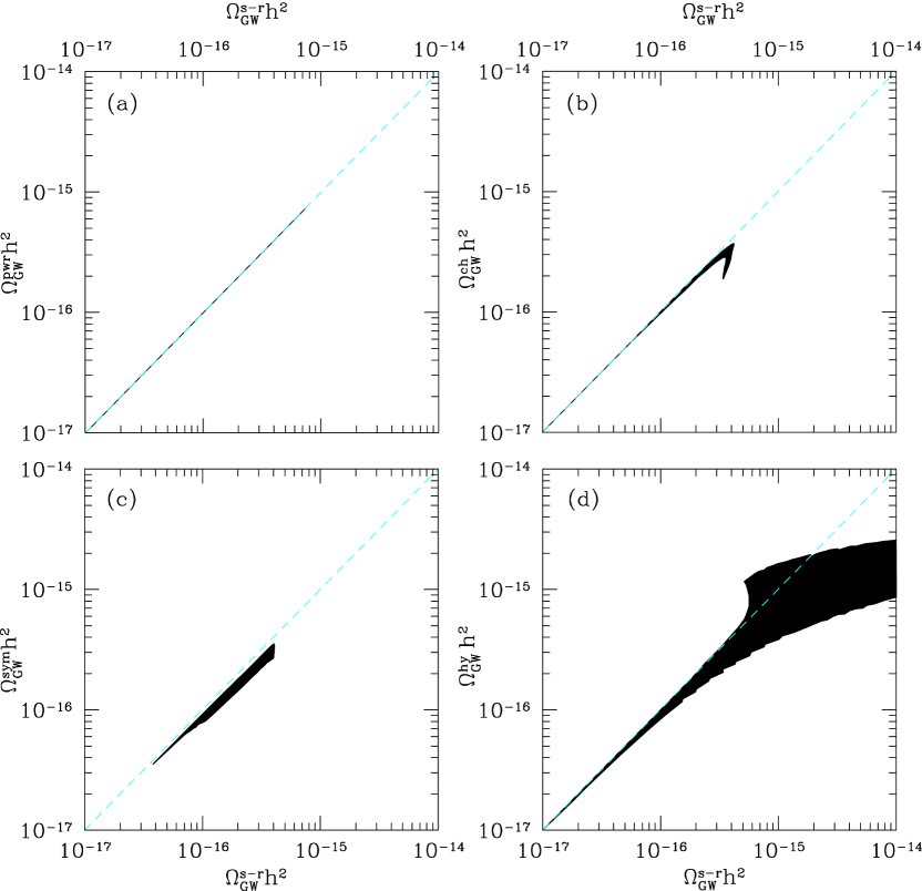
Figure 4: Here we plot the inflationary gravitational-wave background amplitude $\Omega_{\mathrm{GW}}h^{2}$ obtained with the exact inflationary dynamics described in Section IV versus the amplitudes obtained with the power-law approximations (with slow-roll parameters fixed by CMB/LSS observations) given in Section IIb. The panels show results for (a) power-law, (b) chaotic, (c) symmetry-breaking, and (d) hybrid inflation. The regions are models taken from the $n_{s}$–$r$ parameter space in Fig. 1 (and shown in Fig. 3) and the blue dashed curves indicate equality.

However, BBO/DECIGO frequencies are separated from those probed by the CMB/LSS by roughly sixteen orders of magnitude. The inflaton may thus traverse a significant distance, and so it is not obvious that the Taylor expansion approximation that underlies the power-law approximation (even with the running of the spectral index) will remain valid. For example, in Eqs. (12) and (13), the tensor and scalar tilt are written in terms of the first-order slow-roll parameters, while second- and higher-order corrections (e.g., Ref. Stewart and Lyth (1993b)) may be important when extending the power spectrum over large physical scales. Similarly, one must also account for higher-order derivatives of the tilt, beyond the running considered with $\alpha_{s}$ and $\alpha_{t}$. For the calculation performed here, higher order corrections are not important as $\Omega_{\mathrm{GW}}h^{2}$ was directly determined with model parameters describing the inflaton potential, rather than through the power spectrum. Assuming the Taylor approximation is valid, then measurements of $P_{s}$, $n_{s}$, and $r$ at CMB/LSS scales fix the parameters $P_{t}(k_{c})$, $n_{t}$, and $\alpha_{t}$ in Eq. (11), which can then be used to predict $P_{t}(k_{g})\propto\Omega_{\mathrm{GW}}h^{2}$, the IGWB amplitude at BBO/DECIGO scales. An approach based on the Taylor expansion was considered in Ref. Ungarelli et al. (2005) to estimate the GW amplitude at frequencies corresponding to direct detections. Fig. 4 plots the exact IGWB amplitude obtained from the calculation in the previous Section versus that obtained from the power-law approximation. For small IGWB amplitudes, $r=16\epsilon\rightarrow 0$, and so the potentials are very close to flat and the power law tends to be a good approximation, and is indeed a good approximation for the four classes of models we have considered. For power-law inflation, where the power spectra are precisely power laws, the two results are identical. For chaotic and symmetry-breaking inflation, $\epsilon$ becomes large when the IGWB amplitude becomes large, and $\epsilon$ evolves during inflation in such a way that the power-law approximation overestimates the true IGWB amplitude at direct-detection scales. The behavior of hybrid inflation is a bit more subtle. The running of the tensor spectral index is $\alpha_{t}=(r/8)(n_{s}-1+r/8)$ which, for $n_{s}>1-r/8$ can be positive. The (running) power-law would then suggest that $n_{t}$ will become positive at some small distance scale, which cannot be [see Eq. (13)]. The power-law approximation can then overestimate the true IGWB amplitude at BBO/DECIGO scales. On the other hand, in hybrid inflation, unlike chaotic and symmetry-breaking inflation, $\epsilon$ can indeed decrease as inflation proceeds, and so the direct-detection amplitude may also be underestimated by the power-law approximation. Both behaviors are seen in Fig. 4.

It should also be kept in mind that the tensor spectral index $n_{t}$ is most generally different at CMB scales than it is at direct-detection scales, and it is conceivably measurable at both. Determination of $n_{t}$ at both distance scales could therefore distinguish between inflationary models. For example, in power-law inflation, $n_{t}$ remains precisely constant, while it can change by roughly a factor of two for chaotic inflation for models with a directly detectable IGWB. Realistically, though, the tensor spectral indices are generically (although not in full generality) small, and so running of the tensor spectral index will be difficult to measure.

Finally, the four classes of models we have considered are not at all exhaustive, and another inflaton potential could yield a direct-detection IGWB amplitude different from those we have considered here and different from what extrapolation from CMB/LSS would suggest from the power-law approximation. For example, in models with broken scale invariance Starobinsky (1992); Lesgourgues et al. (1998), the direct-detection amplitude could be considerably different.

VI Broken Scale Invariant Spectrum

To demonstrate that direct observations of the IGWB can distinguish between different forms of the inflaton potential, we consider as a toy model the broken scale invariant (BSI) potential, which features a sharp change in the slope of the inflaton potential at some transition scale Starobinsky (1992); Lesgourgues et al. (1998); Polarski (1999). Such models have been invoked to explain, e.g., the paucity of dwarf galaxies observed around the Milky Way Kamionkowski and Liddle (2000); Zentner and Bullock (2002, 2003).

Consider a potential of the form,

$$V(\phi)=V_{0}\times\begin{cases}(1+A\phi),\mathrm{\phi\gtrsim 0}\\ (1+cA\phi),\mathrm{\phi\lesssim 0},\end{cases}$$ (56)

where $V_{0}$ is the overall normalization, $A$ is the slope of the potential at CMB/LSS scales and $c$ parameterizes how the slope changes after the break at $\phi=0$. We allow $\phi_{c}$ to be a free parameter, only requiring that it be before the break in the potential at $\phi=0$. This freedom supposes that field value at which inflation ends is not necessarily determined by the form of the potential in Eq. (56). In order to choose $\phi_{c}$, we place the break (i.e., $\phi=0$) $N_{0}$ $e$-folds from $\phi_{c}$. A natural choice for $N_{0}$ is 10, since we suppose that CMB/LSS scales constrain the inflaton potential from $10^{4}\ \mathrm{Mpc}$ to $1\ \mathrm{Mpc}$. The normalization of the scalar power-spectrum then fixes the normalization $V_{0}$ of the potential through the expression,

$$V_{0}=\frac{3P_{s}(k_{c})}{128}\frac{A^{2}M_{\mathrm{Pl}}^{2}}{(1+A\phi_{c})^{3}}M_{\mathrm{Pl}}^{4}.$$ (57)

We then integrate Eq. (18), assuming the transition at $\phi=0$ has a negligible contribution, between $\phi_{c}$ and $\phi_{g}$ with $N=35$ in order to find $\phi_{g}$. We require that inflation not end before we reach $\phi_{g}$. For $V(\phi)$ as in Eq. (56), we find that inflation ends soon after the field reaches a value, $\phi_{*}=M_{\mathrm{Pl}}/(4\sqrt{\pi})-(cA)^{-1}$. This then places a constraint on the combination $cA$,

$$cA<\frac{4\sqrt{\pi}}{M_{\mathrm{Pl}}\sqrt{1+4(N_{g}-N_{0})}}.$$ (58)

At CMB/LSS scales we find that $\eta(\phi_{c})=0$, and

$$\epsilon(\phi_{c})=\frac{A^{2}M_{\mathrm{Pl}}^{2}}{4A^{2}M_{\mathrm{Pl}}^{2}N_{0}+16\pi}.$$ (59)

From the above expression and Eqs. (12) and (16), we can see explicitly that $n_{s}$ and $r$ only depend on our choice of $N_{0}$ and $A$. At BBO/DECIGO scales we find

$$\Omega_{\mathrm{GW}}h^{2}=4A_{\mathrm{GW}}P_{s}(k_{c})A^{2}M_{\mathrm{Pl}}^{2}\frac{\sqrt{A^{2}c^{2}M_{\mathrm{Pl}}^{2}(N_{0}-N_{g})+4\pi}}{(A^{2}M_{\mathrm{Pl}}^{2}N_{0}+4\pi)^{3/2}},$$ (60)

where $N_{g}$ is the number of $e$-foldings between $\phi_{c}$ and $\phi_{g}$. In order for there to be $N_{g}$ $e$-folds between $\phi_{c}$ and $\phi_{g}$ the slope of the potential cannot be too large, requiring

$$cA\leq\frac{2\sqrt{\pi}}{M_{\mathrm{Pl}}\sqrt{N_{g}-N_{0}}}.$$ (61)

Comparing this to Eq. (58), we find that this constraint is slightly less restrictive. We can see that this amplitude depends not only on $N_{0}$ and $A$ but also on $c$. Therefore, potentials that share approximately the same Taylor expansion at CMB/LSS scales, but different expansions at BBO/DECIGO scales, will produce overlapping observations in the $(n_{s},r)$ plane at CMB/LSS scales and different gravitational-wave amplitudes at BBO/DECIGO scales. With the constraint in Eq. (58), we find that as $c$ increases towards its maximum value (for a fixed $A$), the amplitude of the IGWB changes by an order of magnitude. For example, for $n_{s}=0.9$ and $r=0.27$ we have $1.0\times 10^{-16}\lesssim\Omega_{\mathrm{GW}}h^{2}\lesssim 1.0\times 10^{-15}$; for $n_{s}=0.99$ and $r=3.16\times 10^{-3}$ we have $2.1\times 10^{-18}\lesssim\Omega_{\mathrm{GW}}h^{2}\lesssim 2.1\times 10^{-17}$; and for $n_{s}=1.0$ and $r=3.18\times 10^{-5}$ we have $2.1\times 10^{-20}\lesssim\Omega_{\mathrm{GW}}h^{2}\lesssim 2.1\times 10^{-19}$.

VII Discussion

In this paper we have calculated the gravitational-wave amplitude at direct-detection scales for four classes of inflationary potentials with parameters consistent with current constraints from the CMB and LSS. The gravitational-wave amplitude $\Omega_{\mathrm{GW}}h^{2}$ is proportional to the height $V(\phi_{g})$ of the inflaton potential at the time that direct-detection comoving scales exit the horizon. Our current theoretical understanding does not fix $V(\phi_{g})$; it is constrained to be $V^{1/4}\lesssim 3.4\times 10^{16}$ GeV from the CMB, and it could conceivably be as low as $T\sim 1$ MeV without violating observational constraints. Moreover, detectability of the IGWB with BBO or DECIGO requires $V^{1/4}\gtrsim 10^{15}$ GeV, close to the upper allowed limit. It thus seems, a priori, that detectable models occupy a small region of parameter space.

That said, however, there are indeed constraints to inflationary models that come from the CMB and large-scale structure, notably constraints to the density-perturbation amplitude and spectral index. Fig. 3 indicates that when we go through the exercise of writing down simple functional forms for the inflationary potentials and imposing current constraints, there are large regions of parameter space that lead to directly detectable IGWB amplitudes. In particular, for the symmetry-breaking potential, which looks perhaps like the type of Higgs potentials we might associated with grand unification, current constraints lead to a directly detectable IGWB amplitude.

The promise of detectability traces back to the fact that $\Omega_{\mathrm{GW}}h^{2}\propto V\propto(V^{\prime})^{4/3}$, the last proportionality tracing back to Eqs. (8) and (9) for fixed density-perturbation amplitude $P_{s}$. Thus, if the potential is extremely flat, $V^{\prime}\rightarrow 0$, then the IGWB will be tiny. However, if the potential takes a form in which $V^{\prime}\sim V/\phi$, which seems theoretically natural, then the required density-perturbation amplitude is achieved with $V\sim 10^{(15-16)}$ GeV, the range that produces an accessible IGWB amplitude.

There is of course still plenty of room for inflation to be correct and for the IGWB amplitude to be well below the BBO or DECIGO threshold. For example, in power-law inflation and chaotic inflation, the IGWB amplitude becomes small when $n_{s}\rightarrow 1$; i.e., when scale invariance is achieved which, in these models corresponds to small $V^{\prime}$. On the other hand, a value $n_{s}\rightarrow 1$ does not, more generally, imply a small IGWB amplitude. For example, in hybrid inflation one can have $n_{s}=1$ if $y_{c}^{2}=1/2$ [cf., Eq. (48)], and for $\mu\gtrsim 1.8\,M_{\mathrm{Pl}}$, the potential can reach values at CMB/LSS scales of $V\sim 3\times 10^{16}$ GeV, which even after the decrease to BBO/DECIGO scales remains within reach of detection, as shown in Fig. 3(d).

There may of course be alternatives to inflation, such as cyclic models Steinhardt and Turok (2002) or the pre big-bang model Veneziano (1991); Gasperini and Veneziano (1994); Vernizzi et al. (2001); Veneziano (2000); Brustein et al. (1995); Buonanno et al. (1997), that have completely different IGWB spectra. Although the cyclic model predicts a blue tensor spectrum, which might improve detectability at small scales, BBN constrains the amplitude of the gravitational-wave amplitude to be orders of magnitude below the BBO/DECIGO sensitivities Boyle et al. (2004).

Our conclusion is that direct detection of the IGWB is unlikely without detection with the CMB polarization. Still, direct detection could be extraordinarily valuable even if the IGWB is detected first in the CMB. Direct detection would provide yet another cross-check that the curl component in the CMB polarization is due to gravitational waves, as opposed to some other mechanism (e.g., vector modes, cosmic shear, or foregrounds). Since it occurs on such vastly different distance scales, direct detection can verify that it is a nearly scale-invariant spectrum of gravitational waves, as predicted by inflation, as opposed to some other phenomenon that might only produce large-wavelength gravitational waves. It would provide evidence for the continuation of inflation to distance scales well beyond those implied by the smoothness of the Universe suggested by the successes of BBN. The large lever arm provides an opportunity to discriminate between inflationary models that produce the same CMB/LSS observables. Even within the context of a given inflationary potential, the large lever arm associated with direct detection may allow a measurement of inflationary parameters that may be more precise than those accessible with the CMB/LSS alone. For example, an uncertainty of $10\%$ in $\epsilon$ from the CMB/LSS translates to a $\sim(10^{15})^{0.2}\sim 1000$ uncertainty in the BBO/DECIGO amplitude. Thus, a detection alone, with no better than an order-unity amplitude uncertainty, corresponds to a measurement of $\epsilon$ to roughly 0.02, probably better than is accessible with the CMB/LSS alone. Finally, the deci-Hertz IGWB amplitude counts the number of relativistic degrees of freedom at temperatures a bit above the electroweak symmetry-breaking scale, and may thus be used to probe for new degrees of freedom associated with supersymmetry of some other new physics at the electroweak scale Seto and Yokoyama (2003). The direct search for inflationary gravitational waves may thus be warranted.