Deep echelle spectrophotometry of S 311, a Galactic H ii region located outside the solar circle

Abstract

We present echelle spectrophotometry of the Galactic H ii region S 311. The data have been taken with the Very Large Telescope UVES echelle spectrograph in the 3100 to 10400 Å range. We have measured the intensities of 263 emission lines, 178 are permitted lines of H⁰, D⁰ (deuterium), He⁰, C⁰, C⁺, N⁰, N⁺, O⁰, O⁺, S⁺, Si⁰, Si⁺, Ar⁰ and Fe⁰; some of them are produced by recombination and others mainly by fluorescence. Physical conditions have been derived using different continuum and line intensity ratios. We have derived He⁺, C⁺⁺ and O⁺⁺ ionic abundances from pure recombination lines as well as abundances from collisionally excited lines for a large number of ions of different elements. We have obtained consistent estimations of $t^{2}$ applying different methods. We have found that the temperature fluctuations paradigm is consistent with the $T_{\rm e}$(He i) vs. $T_{\rm e}$(H i) relation for H ii regions, in contrast with what has been found for planetary nebulae. We report the detection of deuterium Balmer lines up to D$\delta$ in the blue wings of the hydrogen lines, which excitation mechanism seems to be continuum fluorescence.

1 Introduction

S 311 —also known as NGC 2467— is an H ii region of the Sharpless catalogue (Sharpless, 1959) which is located outside the solar circle. This nebula forms part of the Puppis I association located at 4.0 kpc from the Sun (Russeil, 2003) and at a Galactocentric distance of 10.43 kpc (assuming a Galactocentric solar distance of 8.0 kpc). (Albert et al.1986) concluded that the radio morphology of S 311 is consistent with blister processes. There are few spectrophotometric studies of S 311 in the literature, most of them forming part of analisys involving several H ii regions (e.g. Hawley, 1978; Peimbert, Torres-Peimbert & Rayo, 1978; Kennicutt et al., 2000). All these works are based on the analysis of collisionally excited lines (hereinafter CELs).

We have taken long-exposure high-spectral-resolution spectra with the Very Large Telescope (VLT) UVES echelle spectrograph to obtain accurate measurements of very faint permitted lines of heavy element ions in S 311. We have determined the physical conditions and the chemical abundances of S 311 with high accuracy. An important improvement in this work is the derivation of C⁺⁺ and O⁺⁺ abundances from several pure recombination lines (hereinafter RLs) of C ii and O ii, making use of high spectral resolution and avoiding the problems of line blending.

Traditionally, the abundance studies for H ii regions have been based on determinations from CELs, whose emissivities are strongly dependent on the temperature variations over the observed volume of the nebula. Alternatively, the emissivities of RLs are almost independent of such variations and are, in principle, more precise indicators of the true chemical abundances of the nebula. The use of high resolution echelle spectrographs has permitted our group to obtain deep high resolution spectra of bright Galactic H ii regions (e.g. Esteban et al., 1998, 1999a; Esteban et al., 1999b, 2004; García-Rojas et al., 2004), and extragalactic H ii regions (e.g. Esteban et al., 2002; Peimbert, 2003); all these works have found that abundance determinations from RLs are systematically larger than those obtained using CELs (the so called abundance discrepancy problem). One of the most probable causes of this abundance discrepancy is the presence of spatial variations or fluctuations in the temperature structure of the nebulae (Torres-Peimbert, Peimbert, & Daltabuit, 1980). Both phenomena can be related due to the different functional dependence of the line emissivities of CELs and RLs on the electron temperature, which is stronger —exponential— in the case of CELs. The temperature fluctuations have been parametrized traditionally by $t^{2}$, the mean square temperature fluctuation of the gas (Peimbert, 1967). We have computed $t^{2}$ values from the comparison of abundances derived using CELs or RLs, and from the temperatures derived from CELs and recombination processes.

The main aims of this work are to present the high-quality spectrophotometric data for S 311 obtained with the ESO Very Large Telescope (VLT), to assess the old-fashioned abundance analysis of S 311 in the literature, calculate C⁺⁺ and O⁺⁺ abundances from recombination lines, and report the detection and measurement of weak deuterium Balmer lines.

In §§ 2 and 3 we describe the observations, the data reduction procedure and the measurement and identification of the emission lines. In § 4 we obtain temperatures and densities using several diagnostic ratios. In § 5 ionic abundances are determined based on CELs, as well as on RLs. In § 6 we discuss the $t^{2}$ results. Total abundances are determined in § 7. In § 8 we discuss the detection of deuterium Balmer lines. Finally, in §§ 9 and  10 we present the discussion and the conclusions, respectively.

2 Observations and Data Reduction

Table 1: Journal of observations.

Telescope	Date	$\Delta\lambda$ (Å)	Exp. time (s)
8.2 m VLT	2003/03/30	3000$-$3900	3$\times$600
”	”	3800$-$5000	60,3$\times$1800
”	”	4750$-$6800	3$\times$600
”	”	6700$-$10400	60,3$\times$1800

The observations were made on 2003 March 30 with the Ultraviolet Visual Echelle Spectrograph, UVES (D’Odorico et al., 2000), at the VLT Kueyen Telescope in Cerro Paranal Observatory (Chile). We used the standard settings in both the red and blue arms of the spectrograph, covering the region from 3100 to 10400 Å . The log of the observations is presented in Table 1.

The wavelength regions 5783–5830 Å and 8540–8650 Å were not observed due to a gap between the two CCDs used in the red arm. There are also five small gaps that were not observed, 9608–9612 Å, 9761–9767 Å, 9918–9927 Å, 10080–10093 Å and 10249–10264 Å, because the five redmost orders did not fit completely within the CCD. We took long and short exposure spectra to check for possible saturation effects.

The slit was oriented east-west and the atmospheric dispersion corrector (ADC) was used to keep the same observed region within the slit regardless of the air mass value. The slit width was set to 3.0$\arcsec$ and the slit length was set to 10$\arcsec$ in the blue arm and to 12$\arcsec$ in the red arm; the slit width was chosen to maximize the S/N ratio of the emission lines and to maintain the required resolution to separate most of the weak lines needed for this project. The effective resolution at a given wavelength is approximately $\Delta\lambda\sim\lambda/8800$. The centre of the slit was placed 126$\arcsec$ south of the main ionizing star HD 64315 (O6e), covering the brightest region of S 311 (see Figure 1). The reductions were made for an area of 3$\arcsec$$\times$8.5$\arcsec$.

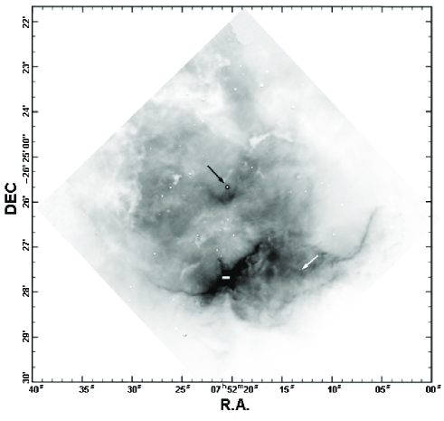
Figure 1: Deep continuum-subtracted H$\alpha$ image of S 311. The image was taken at the Nordic Optical Telescope (2.56m) in the Roque de los Muchachos Observatory, in La Palma (Spain) and is courtesy of A. R. López-Sánchez. The black arrow indicates the position of the ionising star HD 64315. The white arrow indicates the position of the star NGC 2467–12 (see §6) The slit position is indicated as a white horizontal bar.

The spectra were reduced using the IRAF echelle reduction package, following the standard procedure of bias subtraction, aperture extraction, flatfielding, wavelength calibration and flux calibration. The standard stars EG 247, C-32d9927 (Hamuy et al., 1992, 1994) and HD 49798 were observed for flux calibration.

3 Line Intensities and Reddening Correction

Line intensities were measured integrating all the flux in the line between two given limits and over a local continuum estimated by eye. In the cases of line blending, a multiple Gaussian profile fit procedure was applied to obtain the line flux of each individual line. Most of these measurements were made with the SPLOT routine of the IRAF package. In some cases of very tight blends or blends with very bright telluric lines the analysis was performed via Gaussian fitting making use of the Starlink DIPSO software (Howard & Murray, 1990).

Table 2: Observed and reddening-corrected line ratios [F(H$\beta$)=100] and identifications.

$\lambda_{\rm 0}$			$\lambda_{\rm obs}$			err	Notes
(${\rm\AA}$)	Ion	Mult.	(${\rm\AA}$)	$F(\lambda)$a	$I(\lambda)$b	(%)
3187.84	He I	3	3188.45	2.383	4.486	6
3587.28	He I	32	3588.08	0.191	0.294	20
3613.64	He I	6	3614.45	0.276	0.422	15
3634.25	He I	28	3635.08	0.355	0.537	12
3656.11	H I	H35	3658.75	0.070	0.105	:
3658.64	H I	H34	3659.39	0.103	0.154	34
3659.42	H I	H33	3660.26	0.135	0.202	27
3660.28	H I	H32	3661.06	0.180	0.269	21
3661.22	H I	H31	3662.10	0.234	0.350	17
3662.26	H I	H30	3663.04	0.177	0.264	22
3663.40	H I	H29	3664.25	0.210	0.314	19
3664.68	H I	H28	3665.45	0.255	0.380	16
3666.10	H I	H27	3666.91	0.256	0.382	16
3667.68	H I	H26	3668.49	0.270	0.402	15
3669.47	H I	H25	3670.26	0.315	0.470	14
3671.48	H I	H24	3672.27	0.375	0.559	12
3673.76	H I	H23	3674.57	0.381	0.567	12
3676.37	H I	H22	3677.17	0.496	0.739	10
3679.36	H I	H21	3680.16	0.486	0.722	10
3682.81	H I	H20	3683.63	0.545	0.808	9
3686.83	H I	H19	3687.63	0.617	0.914	8
3691.56	H I	H18	3692.36	0.777	1.150	7
3697.15	H I	H17	3697.97	0.900	1.329	7
3703.86	H I	H16	3704.67	1.024	1.504	6
3705.04	He I	25	3705.84	0.407	0.597	11
3711.97	H I	H15	3712.79	1.200	1.756	6
3721.83	[S III]	2F	3722.68	2.156	3.145	5
3721.94	H I	H14
3726.03	[OII]	1F	3726.88	113.36	165.15	4
3728.82	[OII]	1F	3729.63	133.39	194.14	4
3734.37	H I	H13	3735.19	1.812	2.633	5
3750.15	H I	H12	3750.97	2.305	3.330	4
3770.63	H I	H11	3771.47	2.822	4.048	4
3797.90	H I	H10	3798.74	3.721	5.289	4
3819.61	He I	20	3820.47	0.731	1.031	7
3831.66	S II		3832.51	0.026	0.036	29	g
3833.57	He I	62	3834.37	0.117	0.165	10
3835.39	H I	H9	3836.23	5.226	7.338	4
3856.02	Si II	1	3856.97	0.046	0.064	20	e
3856.13	O II	12
3867.48	He I	20	3868.31	0.084	0.117	12
3868.75	[Ne III]	1F	3869.62	3.708	5.152	4
3871.60	He I	60	3872.67	0.076	0.105	14
3888.65	He I	2	3889.50	5.177	7.149	4
3889.05	H I	H8	3889.91	7.991	11.034	4
3920.68	C II	4	3921.47	0.034	0.046	25
3926.53	He I	58	3927.44	0.098	0.134	11
3964.73	He I	5	3965.61	0.668	0.902	4
3967.46	[Ne III]	1F	3968.34	1.149	1.549	4
3970.07	H I	H7	3970.95	11.680	15.728	4
4008.36	[Fe III]	4F	4009.25	0.029	0.039	28
4009.22	He I	55	4010.14	0.125	0.167	9
4026.21	He I	18	4027.10	1.457	1.927	4
4068.60	[S II]	1F	4069.51	1.710	2.227	4
4076.35	[S II]	1F	4077.25	0.598	0.777	4
4100.62	D I	D6	4101.47	0.025	0.032	30
4101.74	H I	H6	4102.64	19.255	24.792	3
4120.82	He I	16	4121.75	0.126	0.161	9
4143.76	He I	53	4144.68	0.220	0.280	6
4153.30	O II	19	4154.18	0.019	0.024	:

Table 2: continued

$\lambda_{\rm 0}$			$\lambda_{\rm obs}$			err	Notes
(${\rm\AA}$)	Ion	Mult.	(${\rm\AA}$)	$F(\lambda)$a	$I(\lambda)$b	(%)
4168.97	He I	52	4169.90	0.035	0.044	24	e
4169.22	O II	19
4267.15	C II	6	4268.11	0.087	0.108	12
4287.40	[Fe II]	7F	4288.35	0.024	0.029	33
4303.61	O II	66	4304.83	0.030	0.036	27
4303.82	O II	53
4339.29	D I	D5	4340.26	0.036	0.044	22
4340.47	H I	H5	4341.42	38.644	46.737	3
4359.34	[Fe II]	7F	4360.32	0.022	0.026	35
4363.21	[O III]	2F	4364.17	0.468	0.562	4
4366.89	O II	2	4367.95	0.077	0.092	13
4368.15	O I	5	4369.22	0.032	0.039	26
4368.25	O I	5
4387.93	He I	51	4388.90	0.439	0.522	4
4437.55	He I	50	4438.52	0.063	0.073	15
4471.48	He I	14	4472.49	3.521	4.056	3
4562.60	Mg I]	1	4563.63	0.138	0.153	8
4571.10	Mg I]	1	4572.13	0.120	0.134	9
4630.54	N II	5	4631.65	0.019	0.021	39
4638.86	O II	1	4639.88	0.026	0.028	30
4641.81	O II	1	4642.85	0.026	0.028	30
4649.13	O II	1	4650.16	0.023	0.025	33
4650.84	O II	1	4651.81	0.023	0.025	33
4654.12	O I	18	4655.05	0.013	0.014	:
4658.10	[Fe III]	3F	4659.16	0.184	0.197	7
4661.63	O II	1	4662.60	0.022	0.024	35
4667.01	[Fe III]	3F	4667.91	0.021	0.022	:
4701.62	[Fe III]	3F	4702.62	0.050	0.052	18
4711.37	[Ar IV]	1F	4712.51	0.012	0.012	:	e
4713.14	He I	12	4714.22	0.394	0.415	4
4754.83	[Fe III]	3F	4755.80	0.041	0.042	21
4769.60	[Fe III]	3F	4770.58	0.019	0.020	36
4777.78	[Fe III]	3F	4778.76	0.015	0.016	:
4814.55	[Fe II]	20F	4815.64	0.018	0.018	:
4815.51	S II	9	4816.67	0.027	0.027	28
4860.03	D I	D4	4861.08	0.085	0.085	18
4861.33	H I	H4	4862.40	100.00	100.00	3
4881.00	[Fe III]	2F	4882.13	0.059	0.059	16
4921.93	He I	48	4923.03	1.117	1.093	4
4924.50	[Fe III]	2F	4925.60	0.020	0.020	38
4924.50	O II	28
4930.50	[Fe III]	1F	4931.63	0.017	0.016	:
4931.32	[O III]	1F	4932.28	0.028	0.027	29
4958.91	[O III]	1F	4960.02	44.315	42.916	3
4985.90	[Fe III]	2F	4986.94	0.142	0.136	12
5006.84	[O III]	1F	5007.96	132.658	126.110	3
5015.68	He I	4	5016.79	2.328	2.207	3
5035.79	[Fe II]	4F	5037.02	0.023	0.022	:
5041.03	Si II	5	5042.25	0.027	0.025	:
5047.74	He I	47	5048.92	0.225	0.211	10
5055.98	Si II	5	5057.12	0.051	0.048	32
5056.31	Si II	5
5191.82	[Ar III]	1F	5192.84	0.056	0.050	30
5197.90	[N I]	1F	5199.12	0.389	0.349	7
5200.26	[N I]	1F	5201.47	0.330	0.296	8
5270.30	[Fe III]	1F	5271.70	0.124	0.108	16
5517.71	[Cl III]	1F	5518.91	0.566	0.461	6
5537.88	[Cl III]	1F	5539.06	0.437	0.354	7
5577.34	[O I]	3F	5578.56	0.072	0.057	25
5754.64	[N II]	3F	5755.89	1.315	0.992	4

Table 2: continued

$\lambda_{\rm 0}$			$\lambda_{\rm obs}$			err	Notes
(${\rm\AA}$)	Ion	Mult.	(${\rm\AA}$)	$F(\lambda)$a	$I(\lambda)$b	(%)
5875.64	He I	11	5876.96	15.602	11.343	4
5978.83	Si II	4	5980.31	0.076	0.054	24
6046.44	O I	22	6047.77	0.034	0.024	:
6300.30	[O I]	1F	6301.75	3.512	2.307	4
6312.10	[S III]	3F	6313.48	2.057	1.348	4
6363.78	[O I]	1F	6365.24	1.258	0.815	5
6371.36	Si II	2	6372.85	0.064	0.041	27
6548.03	[N II]	1F	6549.54	42.523	26.484	4
6561.04	D I	D3	6562.43	0.321	0.200	9
6562.82	H I	H3	6564.26	458.723	284.845	4
6578.05	C II	2	6579.49	0.196	0.121	12
6583.41	[N II]	1F	6584.93	131.646	81.408	4
6678.15	He I	46	6679.64	5.374	3.263	4
6716.47	[S II]	2F	6717.97	43.847	26.434	4
6730.85	[S II]	2F	6732.35	39.503	23.752	4
6933.91	He I	1/13	6935.57	0.017	0.010	:	g
6989.45	He I	1/12	6991.12	0.024	0.014	:
7002.23	O I	21	7003.53	0.179	0.103	9	c
7065.28	He I	10	7066.81	3.780	2.149	5
7092.19	C I]		7093.57	0.039	0.022	32
7093.97	[Fe II]		7095.54	0.013	0.007	:	g
7105.85	Si I	70	7107.13	0.029	0.016	:	g
7111.47	C I		7113.06	0.034	0.019	37	g
7135.78	[Ar III]	1F	7137.37	17.966	10.102	5
7155.14	[Fe II]	14F	7156.81	0.029	0.016	:
7160.58	He I	1/10	7162.20	0.048	0.027	27
7231.34	C II	3	7232.89	0.070	0.039	19
7236.19	C II	3	—	—	—	-	c
7281.35	He I	45	7282.98	1.055	0.580	5
7298.05	He I	1/9	7299.71	0.039	0.021	33
7318.39	[O II]	2F	7320.69	1.985	1.085	4
7319.99	[O II]	2F	7321.77	6.024	3.293	5
7329.66	[O II]	2F	7331.33	3.311	1.807	5
7330.73	[O II]	2F	7332.41	3.133	1.710	5
7377.83	[Ni II]	2F	7379.55	0.019	0.010	:
7423.64	N I	3	7425.40	0.026	0.014	:
7442.30	N I	3	7444.02	0.050	0.027	26
7468.31	N I	3	7470.14	0.156	0.083	10
7499.85	He I	1/8	7501.53	0.066	0.035	20
7706.74	O I	42	7708.80	0.036	0.019	35
7751.10	[Ar III]	2F	7752.84	4.854	2.500	5
7782.10	Ca I]		7784.06	0.073	0.038	18
7790.60	Ar I		7792.83	0.064	0.033	21
7801.56	[Cr II]		7803.60	0.051	0.026	25
7816.13	He I	1/7	7817.90	0.106	0.054	14
7837.85	[Co I]		7839.58	0.105	0.053	14
7862.75	Fe II]		7864.55	0.023	0.012	:	g
7875.99	[P II]	1D-1S	7877.68	0.066	0.033	20
7959.70	Co II]		7961.62	0.109	0.055	13	g
8046.80	Si I	73	8048.32	0.048	0.024	27	g
8116	He I	4/16	8116.93	0.008	0.004	:
8150.57	Si I	20	8152.52	0.077	0.038	19
8184.85	N I	2	8186.78	0.029	0.014	:
8188.01	N I	2	8189.93	0.078	0.038	18
8200.36	N I	2	8202.33	0.017	0.008	:
8210.72	N I	2	8212.65	0.036	0.017	35
8216.28	N I	2	8218.25	0.085	0.042	16
8223.14	N I	2	8225.03	0.095	0.046	15
8243.70	H I	P43	8245.54	0.068	0.033	20
8245.64	H I	P42	8247.66	0.094	0.045	15

Table 2: continued

$\lambda_{\rm 0}$			$\lambda_{\rm obs}$			err	Notes
(${\rm\AA}$)	Ion	Mult.	(${\rm\AA}$)	$F(\lambda)$a	$I(\lambda)$b	(%)
8247.73	H I	P41	8249.60	0.090	0.044	16
8249.97	H I	P40	8251.80	0.081	0.039	17
8252.40	H I	P39	8254.35	0.130	0.063	12
8255.02	H I	P38	8256.88	0.104	0.050	14
8257.85	H I	P37	8259.72	0.104	0.050	14
8260.93	H I	P36	8262.76	0.112	0.054	13
8264.28	H I	P35	8266.18	0.159	0.077	10
8266.40	Ar I		8268.32	0.092	0.045	15
8267.94	H I	P34	8269.78	0.152	0.074	10
8271.93	H I	P33	8273.63	0.086	0.041	16	d
8276.31	H I	P32	—	—	—	–	c
8281.12	H I	P31	8282.85	0.270	0.130	8	c
8286.43	H I	P30	—	—	—	–	c
8292.31	H I	P29	8294.22	0.177	0.085	9
8298.83	H I	P28	8300.72	0.252	0.121	8
8306.11	H I	P27	8307.94	0.286	0.138	7
8314.26	H I	P26	8316.18	0.301	0.145	7
8323.42	H I	P25	8325.28	0.339	0.162	7
8333.78	H I	P24	8335.63	0.434	0.207	6
8334.75	Fe II]		8336.68	0.190	0.091	9	g
8345.55	H I	P23	8347.42	0.423	0.202	6
8359.00	H I	P22	8360.80	0.629	0.299	6
8374.48	H I	P21	8376.33	0.549	0.260	6
8387.77	Fe I		8389.62	0.095	0.045	15	g
8392.40	H I	P20	8394.24	0.634	0.299	6
8395.98	Ca I]		8397.84	0.059	0.028	23	c, g
8413.32	H I	P19	8415.20	0.713	0.336	6	c
8437.96	H I	P18	8439.85	0.818	0.383	6
8446.25	O I	4	8448.41	0.823	0.384	6
8446.36	O I	4
8446.76	O I	4	8448.93	0.056	0.026	24
8451.00	He I	6/17	8453.21	0.043	0.020	30
8459.32	[Cr II]		8461.26	0.193	0.090	9
8467.25	H I	P17	8469.15	0.936	0.435	6
	?		8477.02	0.032	0.015	39
8486.	He I	6/16	8488.26	0.034	0.016	37
8502.48	H I	P16	8504.33	3.337	1.538	6	c
8518.04	He I	2/8	8520.05	0.076	0.035	18
8528.99	He I	6/15	8530.87	0.060	0.027	22	c
8665.02	H I	P13	8666.95	2.136	0.947	6
8680.28	N I	1	8682.31	0.064	0.028	21
8683.40	N I	1	8685.38	0.152	0.067	11
8686.15	N I	1	8688.20	0.044	0.020	29
8703.25	N I	1	8705.22	0.051	0.022	26	c
8711.70	N I	1	8713.75	0.048	0.021	27
8718.83	N I	1	8720.90	0.029	0.013	:
8727.13	[C I]		8729.19	0.470	0.205	7
8733.43	He I	6/12	8735.41	0.074	0.032	18
8750.47	H I	P12	8752.44	2.672	1.161	6
8776.77	He I	4/9	8778.70	0.074	0.032	18
8845.38	He I	6/11	8847.36	0.100	0.043	15
8850.62	Fe I]		8852.74	0.142	0.060	11	g
8862.79	H I	P11	8864.76	3.597	1.525	6
8888.71	Fe I]		8890.93	0.082	0.035	17	g
8893.87	V I]		8895.90	0.203	0.086	9	c,g
8914.77	He I	2/7	8916.58	0.062	0.026	22
8946.05	Fe II]		8948.25	0.088	0.037	16	g
8996.99	He I	6/10	8998.95	0.146	0.060	12
9014.91	H I	P10	9016.97	4.278	1.764	6	d
9019.14	Fe I]		9021.38	0.235	0.097	9	g

Table 2: continued

$\lambda_{\rm 0}$			$\lambda_{\rm obs}$			err	Notes
(${\rm\AA}$)	Ion	Mult.	(${\rm\AA}$)	$F(\lambda)$a	$I(\lambda)$b	(%)
9019.14	Ca I]
9029.07	Fe I]		9031.34	0.145	0.060	11	g
9063.29	He I	4/8	9065.18	0.222	0.091	9
9068.90	[S III]	1F	9070.92	55.891	22.855	6
9094.83	C I		9096.98	0.139	0.056	12	g
9111.83	Ca I]		9113.95	0.048	0.020	27	g
9113.60	Fe I]		9115.67	0.108	0.044	14	g
9123.60	[Cl II]		9125.72	0.225	0.091	9
9162.65	Ni II]		9164.72	0.047	0.019	28	g
9210.28	He I	6/9	9212.41	0.189	0.076	10
9226.62	[Fe II]		9228.58	0.088	0.036	16	g
9229.01	H I	P9	9231.11	6.898	2.770	6
9463.57	He I	1/5	9465.71	0.286	0.113	8
9504.54	C I]		9506.97	0.127	0.050	12	g
9526.16	He I	6/8	9528.46	0.362	0.143	8
9530.60	[S III]	1F	9533.12	156.202	61.749	5
9545.97	H I	P8	9548.13	7.956	3.144	7	d
9702.62	He I	75	9705.23	0.130	0.051	12	c
9824.13	[C I]	1F	9826.49	0.986	0.389	7
9850.24	[C I]	1F	9852.56	2.766	1.091	7
9876.67	Fe I]		9879.00	0.233	0.092	9	g
10027.70	He I	6/7	10029.98	0.595	0.235	7
10049.37	H I	P7	10051.64	17.935	7.086	7
10286.70	[S II]	3F	10288.95	1.978	0.782	7
10320.49	[S II]	3F	10322.75	2.235	0.884	7
10336.41	[S II]	3F	10338.96	3.066	1.212	7

^a

Where $F$ is the observed flux in units of $100.00=3.703\times 10^{-13}$ ergs cm^-2 s^-1.

^b

Where $I$ is the dereddened flux, in units of $100.00=1.616\times 10^{-12}$ ergs cm^-2 s^-1 and assuming C(H$\beta$)=0.64 dex.

^c

Affected by telluric emission lines.

^d

Affected by atmospheric absorption bands.

^e

Affected by internal reflections or charge transfer in the CCD.

^f

Blend with an unknown line.

^g

Dubious identification.

Table 2 presents the emission line intensities of S 311. The first and fourth columns list the adopted laboratory wavelength, $\lambda_{0}$, and the observed wavelength in the heliocentric framework, $\lambda$. The second and third columns give the ion and the multiplet number, or series for each line. The fifth and sixth columns give the observed flux relative to H$\beta$, $F(\lambda$), and the flux corrected for reddening relative to H$\beta$, $I(\lambda$). The seventh column gives the fractional error (1$\sigma$) in the line intensities (see García-Rojas et al., 2004, for details in error analysis).

A total of 263 emission lines were measured; of them 178 are permitted, 65 are forbidden and 19 are semiforbidden (see Table 2). Two H i Paschen lines and one C ii line are blended with telluric lines, making impossible their measurement. Several other lines were strongly affected by atmospheric features in absorption, by internal reflections or charge transfer in the CCD, rendering their intensities unreliable. Also, 23 lines are dubious identifications and one emission line could not be identified in any of the available references. Those lines are indicated in Table 2.

The identification and adopted laboratory wavelengths of the lines were obtained following several previous identifications in the literature (see García-Rojas et al., 2004; Esteban et al., 2004, and references therein)

We have assumed the standard extinction for the Milky Way (R_v=3.1) parametrized by Seaton (1979). We have derived a logarithmic interstellar extinction coefficient of $c(H\beta)$=0.64 $\pm$ 0.04 dex was determined by fitting the observed $I$(H Balmer lines)/$I$(H$\beta$) ratios (from H16 to H$\beta$) and $I$(H Paschen lines)/$I$(H$\beta$) (from P22 to P7), to the theoretical ones computed by Storey & Hummer (1995) for $T_{\rm e}$ = 10000 K and $n_{\rm e}$ = 1000 cm^-3 (see below). H i lines affected by blends or atmospheric absorption were not considered. The derived value of $c(H\beta)$ is in very good agreement with previous determinations in the same nebula: Hawley (1978) derived $c(H\beta)$=0.61 and 0.67 for two slit positions with offsets of 96$\arcsec$ north and 96$\arcsec$ north, 35$\arcsec$ west respectively from our slit position. Furthermore, Peimbert, Torres-Peimbert & Rayo (1978) derived $c(H\beta)$=0.6 and 0.7 for slit positions 33$\arcsec$ north, 12$\arcsec$ west and 33$\arcsec$ north, 106$\arcsec$ west, respectively. These last authors used the Whitford (1958) extinction law, which is almost coincident with the one we have adopted. Moreover, Kennicutt et al. (2000), derived a value of $c(H\beta)$=0.67 using the average interstellar reddening curve from Cardelli, Clayton & Mathis (1989). Shaver et al. (1983) observed two positions in S 311, one of them (position 2), almost coincident with our slit position. They derived $c(H\beta)$=0.5 and 0.7 for their positions 1 and 2 respectively. We can conclude then that apparently there are no significant variations of the extinction inside S 311.

4 Physical Conditions

The large number of emission lines identified and measured in the spectra allows us the derivation of physical conditions using different emission line ratios. The temperatures and densities are presented in Table 3. Most of the determinations were carried out with the IRAF task TEMDEN of the package NEBULAR (Shaw & Dufour, 1995).

The methodology followed for the derivation of $n_{\rm e}$ and $T_{\rm e}$ has been described in a previous paper (i.e. García-Rojas et al., 2004). In the case of electron densities, ratios of CELs of several ions have been used. The lastest version of NEBULAR (February 2004) uses the transition probabilities recommended by Wiese et al. (1996) and the collision strengths of McLaughlin & Bell (1993) for the [O ii] $\lambda$3729/$\lambda$3726 doublet ratio. These atomic data yield electron densities systematically lower than those deduced from the [S ii] $\lambda$6716/$\lambda$6731 doublet ratio (see Esteban et al., 2004; García-Rojas et al., 2004). Following the arguments of Copetti & Writzl (2002) and Wang et al. (2004) we have adopted the transition probabilities from Zeippen (1982) and the collision strengths from Pradhan (1976) for the [O ii] $\lambda$3729/$\lambda$3726 doublet ratio, which give electron densities that are in good agreement with the other density indicators. We have derived the [Fe iii] density from the intensity of the 6 brightest lines lines, which have errors less than 30 % and seem not to be affected by line blending, together with the computations of Rodríguez (2002). All the computed values of $n_{\rm e}$ are consistent within the errors (see Table 3).

Table 3: Plasma Diagnostic.

Parameter	Line	Value
$N_{\rm e}$ (cm-3)	[N i] ($\lambda$5198)/($\lambda$5200)	590${}^{+260}_{-200}$
	[O ii] ($\lambda$3726)/($\lambda$3729)	260 $\pm$ 110
	[S ii] ($\lambda$6716)/($\lambda$6731)	360${}^{+140}_{-120}$
	[Fe iii]	390 $\pm$ 220
	[Cl iii] ($\lambda$5518)/($\lambda$5538)	550${}^{+650}_{-550}$
	$N_{\rm e}$ (adopted)	310 $\pm$ 80
$T_{\rm e}$ (K)	[N ii] ($\lambda$6548+$\lambda$6583)/($\lambda$5755)	9500 $\pm$ 250a
	[S ii] ($\lambda$6716+$\lambda$6731)/($\lambda$4069+$\lambda$4076)	7200 ${}^{+750}_{-600}$
	[O ii] ($\lambda$3726+$\lambda$3729)/($\lambda$7320+$\lambda$7330)	9800 $\pm$ 600a
	$T_{\rm e}$ (low)	9550 $\pm$ 250
	[O iii] ($\lambda$4959+$\lambda$5007)/($\lambda$4363)	9000 $\pm$ 200
	[Ar iii] ($\lambda$7136+$\lambda$7751)/($\lambda$5192)	8800 ${}^{+700}_{-850}$
	[S iii] ($\lambda$9069+$\lambda$9532)/($\lambda$6312)	9300 $\pm$ 350
	$T_{\rm e}$ (high)	9050 $\pm$ 200
	He i	8750 $\pm$ 500
	Balmer line/cont.	9500 $\pm$ 900
	Paschen line/cont.	8700 $\pm$ 1100

^a

Recombination contribution on the auroral lines has been taken into account (see text)

A weighted mean of $n_{\rm e}$(O ii), $n_{\rm e}$(Fe iii), $n_{\rm e}$(Cl iii) and $n_{\rm e}$(S ii) has been used to derive $T_{\rm e}$(N ii), $T_{\rm e}$(O iii), $T_{\rm e}$(Ar iii) and $T_{\rm e}$(S iii), and iterated until convergence. So, for all the species we have adopted $n_{\rm e}$=310 $\pm$ 80 cm^-3. We have excluded $n_{\rm e}$(N i) from the average because this ion is representative of the very outer part of the nebula, and probably does not coexist with most of the other ions.

Electron temperatures have been derived from the ratio of CELs of several ions and making use of NEBULAR routines. In the case of $T_{\rm e}$(S iii) instead of using the collision strengths of Galavís, Mendoza & Zeippen (1995), included by default in NEBULAR, we have used the ones by Tayal & Gupta (1999). The last set of collision strengths gives $T_{\rm e}$(S iii) values more consistent with the rest of temperature determinations. Table 4 shows the atomic data that we have changed in the last version of NEBULAR.

Table 4: Atomic data used for some selected ions.

Ion	Coll. Strengths	Trans. Probability
O+	Pradhan (1976)	Zeippen (1982)
S+	Keenan et al. (1996)	Keenan et al. (1993)
S++	Tayal & Gupta (1999)	Mendoza & Zeippen (1982)

To obtain $T_{\rm e}$(O ii) it is necessary to subtract the contribution to $\lambda\lambda$7320+7330 due to recombination; Liu et al. (2000) find that the contribution to the intensities of the [O ii] $\lambda\lambda$ 7319, 7320, 7331, and 7332 lines due to recombination can be fitted in the range 0.5$\leq$T/10⁴$\leq$1.0 by:

$$\frac{I_{R}(7320+7330)}{I({\rm H\beta})}=9.36\times(T_{4})^{0.44}\times\frac{{\rm{O}}^{++}}{{\rm{H}}^{+}},$$ (1)

where $T_{4}$=$T$/10⁴. With this equation we estimate a contribution of approximately 2% to the observed line intensities.

Liu et al. (2000) also determined that the contribution to the intensity of the $\lambda$ 5755 [N ii] line due to recombination can be estimated from:

$$\frac{I_{R}(5755)}{I({\rm H\beta})}=3.19\times(T_{4})^{0.30}\times\frac{{\rm N}^{++}}{{\rm H}^{+}},$$ (2)

in the range 0.5$\leq$ $T$/10⁴$\leq$2.0. We have obtained a contribution of recombination of about 0.5%, that does not affect significantly the temperature determination.

Figure 2: Section of the echelle spectrum including the Balmer (top) and the Paschen (bottom) limits (observed fluxes).

Figure 2 shows the spectral regions near the Balmer and the Paschen limits. The discontinuities can be easily appreciated. They are defined as $I_{c}(Bac)=I_{c}(\lambda 3646^{-})-I_{c}(\lambda 3646^{+})$ and $I_{c}(Pac)=I_{c}(\lambda 8203^{-})-I_{c}(\lambda 8203^{+})$ respectively. The high spectral resolution of the spectra permits to measure the continuum emission in zones very near de discontinuity, minimizing the possible contamination of other continuum contributions. We have obtained power-law fits to the relation between $I_{c}(Bac)/I(Hn)$ or $I_{c}(Pac)/I(Pn)$ and $T_{\rm e}$ for different $n$ corresponding to different observed lines of both series. The emissivities as a function of electron temperature for the nebular continuum and the H i Balmer and Paschen lines have been taken from Brown & Mathews (1970) and Storey & Hummer (1995) respectively. The $T_{e}(Bac)$ adopted is the average of the values using the lines from $H\alpha$ to H 10 (the brightest ones). In the case of $T_{e}(Pac)$, the adopted value is the average of the individual temperatures obtained using the lines from P 7 to P 13 (the brightest lines of the series), excluding P 8 and P 10 because their intensity seems to be affected by sky absorption.

Peimbert, Peimbert & Luridiana (2002) developed a method to derive the helium temperature, $T_{\rm e}$(He i), in the presence of temperature fluctuations. Assuming a 2-zone ionization scheme and the formulation of Peimbert, Peimbert & Luridiana (2002) we have derived $T_{\rm e}$(He i)=8750 $\pm$ 500 K, which is highly consistent with $T_{\rm e}$(H i) assumed above.

We have assumed a 2-zone ionization scheme for the derivation of ionic abundances (see § 5). We have adopted the average of electron temperatures obtained from [N ii] and [O ii] lines as representative for the low ionization zone, and the average of the values obtained from [O iii], [Ar iii] and [S iii] lines for the high ionization zone (see Table 3).

5 Ionic Abundances

5.1 He⁺ abundance

Table 5: He⁺ abundance.

Line	He+/H+ a
3819.61	775 $\pm$ 54
3888.65	759 $\pm$ 30
3964.73	825 $\pm$ 33
4026.21	818 $\pm$ 33
4387.93	837 $\pm$ 34
4471.09	792 $\pm$ 24
4713.14	821 $\pm$ 33
4921.93	800 $\pm$ 32
5875.64	780 $\pm$ 31
6678.15	793 $\pm$ 32
7065.28	770 $\pm$ 38
7281.35	835 $\pm$ 42
Adopted	795 $\pm$ 9b

^a

In units of 10^-4, for $\tau_{3889}$=2.52 $\pm$ 0.44, and $t^{2}$=0.034 $\pm$ 0.010. Uncertainties correspond to line intensity errors.

^b

It includes all the relevant uncertainties in emission line intensities, $n_{\rm e}$, $\tau_{3889}$ and $t^{2}$.

We have measured 50 He i emission lines identified in our spectra. These lines arise mainly from recombination but they can be affected by collisional excitation and self-absorption effects. We have determined the He⁺/H⁺ ratio using the effective recombination coefficients of Storey & Hummer (1995) for H i and those of Smits (1996) and Benjamin, Skillman & Smits (1999) for He i. The collisional contribution was estimated from Sawey & Berrington (1993) and Kingdon & Ferland (1995), and the optical depths in the triplet lines were derived from the computations by Benjamin, Skillman & Smits (2002). From a maximum likelihood method (e.g. Peimbert, Peimbert & Ruiz, 2000), using $n_{\rm e}$=310 $\pm$ 80 cm^-3 and $T$(O ii+iii)=9600 $\pm$ 450 K (see § 6), we have obtained He⁺/H⁺=0.0795 $\pm$ 0.0009, $\tau_{3889}$=2.52 $\pm$ 0.44, and $t^{2}$=0.034 $\pm$ 0.010. In Table 5 we have included the He⁺/H⁺ ratios we have obtained for the individual He i lines not affected by line blending and with the highest signal-to-noise ratio. We have excluded He i $\lambda$5015 for the same reasons outlined by Esteban et al. (2004). We have done a $\chi^{2}$ optimization of the values in the table, and we have obtained a $\chi^{2}$ parameter of 8.15, which indicates a reasonable goodness of the fit for a system with nine degrees of freedom.

5.2 Ionic Abundances from CELs

Ionic abundances of N⁺, O⁺, O⁺⁺, Ne⁺⁺, S⁺, S⁺⁺, Cl⁺, Cl⁺⁺, Ar⁺⁺ and Ar³⁺ have been determined from CELs, using the IRAF package NEBULAR (except for Cl⁺, see García-Rojas et al., 2004). Additionally, we have determined the ionic abundances of Fe⁺⁺ following the methods and data discussed in García-Rojas et al. (2004). Ionic abundances are listed in Table  6 and correspond to the mean value of the abundances derived from all the individual lines of each ion observed (weighted by their relative intensities).

To derive the abundances for $t^{2}$ = 0.038 (see § 6) we used the abundances for $t^{2}$=0.00 and the formulation of Peimbert (1967) and Peimbert & Costero (1969) for $t^{2}>$0.00. To derive abundances for other $t^{2}$ values it is possible to interpolate or extrapolate the values presented in Table 6.

Table 6: Ionic abundances from collisionally excited lines^a.

Ion	$t^{2}$=0.000	$t^{2}$=0.038 $\pm$ 0.007
N0	5.74 $\pm$ 0.06	5.88 $\pm$ 0.07
N+	7.25 $\pm$ 0.05	7.38 $\pm$ 0.06
O0	6.74 $\pm$ 0.06	6.87 $\pm$ 0.06
O+	8.26 $\pm$ 0.07	8.40 $\pm$ 0.08
O++	7.81 $\pm$ 0.04	8.05 $\pm$ 0.06
Ne++	6.81 $\pm$ 0.05	7.07 $\pm$ 0.07
S+	6.03 $\pm$ 0.05	6.15 $\pm$ 0.06
S++	6.68 $\pm$ 0.07	6.95 $\pm$ 0.09
Cl+	4.56 $\pm$ 0.05	4.67 $\pm$ 0.05
Cl++	4.85 $\pm$ 0.05	5.08 $\pm$ 0.05
Ar++	6.08 $\pm$ 0.04	6.28 $\pm$ 0.06
Ar3+	3.42${}^{+0.18}_{-0.30}$	3.66${}^{+0.18}_{-0.30}$
Fe++	5.05 $\pm$ 0.06	5.30 $\pm$ 0.08

^a

In units of 12+log(X^m/H⁺).

Many [Fe ii] lines have been identified in our spectra, but all of them are severely affected by fluorescence effects (Rodríguez, 1999; Verner et al., 2000). The only [Fe ii] line in the spectral range 3100 ${\rm\AA}$ to 10400 ${\rm\AA}$ which is not affected by fluorescence effects is the [Fe ii] $\lambda 8617$ ${\rm\AA}$ line, but unfortunately it is in one of our observational gaps. We have measured [Fe ii] $\lambda 7155$, a line which is not much affected by fluorescence effects (Verner et al., 2000), but it has a high observational error. Therefore, it was no possible to derive a reliable value of the Fe⁺/H⁺ ratio. The calculations for Fe⁺⁺ have been done with a 34 level model-atom that uses the collision strengths of Zhang (1996) and the transition probabilities of Quinet (1996). We have used 6 [Fe iii] lines that do not seem to be affected by line-blending and with errors less than 30 %. We find a mean value and a standard deviation of Fe⁺⁺/H⁺=(1.115 $\pm$ 0.153)$\times$10^-7. Adding errors in $T_{\rm e}$ and $n_{\rm e}$ we finally obtain 12+log(Fe⁺⁺/H⁺)=5.05 $\pm$ 0.06. The value of the Fe⁺⁺ abundance for t${}^{2}>$0.00 is also shown in Table  6.

5.3 Ionic Abundances from Recombination Lines

Table 7: C⁺⁺/H⁺ abundance ratio from C ii lines

		$I$($\lambda$)/$I$(H$\beta$)	C++/H+ ($\times$10-5)
Mult.	$\lambda_{0}$	($\times$10-2)	A	B
2	6578.05a	0.121 $\pm$ 0.015	129 $\pm$ 15	23 $\pm$ 3
3	7231.12	0.038 $\pm$ 0.007	1037 $\pm$ 197	15 $\pm$ 3
4	3920.68	0.046 $\pm$ 0.012	400 $\pm$ 100	130 $\pm$ 33
6	4267.26	0.108 $\pm$ 0.013	10 $\pm$ 1	10 $\pm$ 1
	Adopted		10 $\pm$ 1

^a

Affected by a telluric emission line

Table 8: O⁺⁺/H⁺ ratio from O ii permitted lines^a

		$I$($\lambda$)/$I$(H$\beta$)	O++/H+ ($\times$10-5)b
Mult.	$\lambda_{0}$	($\times$10-2)	A	B	C
1	4638.85	0.028 $\pm$ 0.008	14 $\pm$ 4	14 $\pm$ 4	–
	4641.81	0.028 $\pm$ 0.008	13 $\pm$ 4	12 $\pm$ 4	–
	4649.14	0.025 $\pm$ 0.008	13 $\pm$ 4	12 $\pm$ 4	–
	4650.84	0.025 $\pm$ 0.008	11 $\pm$ 4	11 $\pm$ 4	–
	4661.64	0.024 $\pm$ 0.008	10 $\pm$ 4	10 $\pm$ 4	–
	Sum		12 $\pm$ 1	12 $\pm$ 1	–
2	4366.89	0.092 $\pm$ 0.012	25 $\pm$ 3	18 $\pm$ 2	–
19	4153.30	0.024:	794:/31:	28:/28:	28:/29:
	Adopted		12 $\pm$ 1

^a

Only lines with intensity uncertainties lower than 40 % have been considered

^b

Abundances of multiplet 1 have been corrected from NLTE effects (see text)

We have measured a large number of permitted lines of heavy element ions such as O i, O ii, C i, C ii, S ii, N i, N ii, Ar i, Si i, Si ii, and Fe i most of them detected for the first time in S 311. Those permitted lines produced by recombination can give accurate determinations of ionic abundances because their intensities depend weakly on electron temperature and density. Unfortunately most of the permitted lines are affected by fluorescence effects or are blended with telluric emission lines making their intensities unreliable; also Ruiz et al. (2003) have shown that, to determine the abundances, it is important to measure all the lines of a multiplet, because for low densities there could be an anomalous distribition of the line intensities within the multiplet. Detailed discussions on the mechanism of formation of the permitted lines are in Esteban et al. (1998, and references therein); Esteban et al. (2004, and references therein).

Figure 3: Section of the echelle spectrum showing the lines of multiplet 1 of O ii (observed fluxes).

We have been able of measuring ionic abundance ratios of O⁺⁺/H⁺ and C${}^{++}/$H⁺ from pure recombination O ii and C ii lines respectively, from multiplet 1 for O ii (see Figure 3) and from multiplet 6 for C ii [see Figure 1 of Esteban et al. (2005)]. We have computed the abundances for $T_{\rm e}$(High)=9050 K and $n_{\rm e}$=310 cm^-3. Atomic data and methodology for the C abundance are the same as in García-Rojas et al. (2004). For the Multiplet 1 of O II it has been shown that for densities $n_{e}$ $<$ 10000 cm^-3 the upper levels of the transition are not in LTE, and if one uses only one line to determine the abundances one can have errors as large as a factor of 4 (Ruiz et al., 2003); instead we used the prescription presented by Peimbert, Peimbert & Ruiz (2005) to calculate those populations; these abundances show very good agreement among themselves and with the abundance determined using the sum of all the lines, “Sum”, that is not expected to be affected by this effect. Tables 7 and 8 show the abundance ratios.

6 Temperature variations

It is well known that under the assumption of a constant temperature, RLs of heavy element ions yield higher abundance values relative to hydrogen than CELs in H ii regions (e.g. Peimbert, Storey & Torres-Peimbert, 1993; Esteban et al., 1998; Esteban, 2002; Esteban et al., 2004; García-Rojas et al., 2004; Tsamis et al., 2003, and references therein). Torres-Peimbert, Peimbert, & Daltabuit (1980) proposed the presence of spatial temperature fluctuations (parametrized by $t^{2}$) as the cause of this discrepancy, because CELs and RLs emissivities have different dependences on the electron temperature. On the other hand, Peimbert (1971) proposed that there is a dichotomy between $T_{\rm e}$ derived from the [O iii] lines and from the hydrogen recombination continuum discontinuities, which is strongly correlated with the discrepancy between CEL and RL abundances, so the comparison between electron temperatures obtained from both methods is an additional indicator of $t^{2}$. A complete formulation of temperature fluctuations has been developed by Peimbert (1967), Peimbert & Costero (1969) and Peimbert (1971). We have assumed a two-zone ionization scheme, and we have followed the re-formulation of Peimbert, Peimbert & Ruiz (2000) and Peimbert, Peimbert & Luridiana (2002) to derive the value of $t^{2}$ comparing $T_{\rm e}$($Bac$) and $T_{\rm e}$($Pac$) with the combination of $T_{\rm e}$([O ii]) and $T_{\rm e}$([O iii]), $t^{2}$($Bac-FL$) and $t^{2}$($Pac-FL$), respectively, using equation (A1) of Peimbert, Peimbert & Luridiana (2002). Table 9 shows the different $t^{2}$ values obtained as well as the adopted value, $t^{2}$=0.038 $\pm$ 0.007 which is the weighted average of O⁺⁺ and He⁺ values which are rather consistent and show the lowest uncertainties.

Table 9: $t^{2}$ parameter

Method	$t^{2}$
O++ (R/C)	0.040 $\pm$ 0.008
He+	0.034 $\pm$ 0.010
Bac–FL	0.002 $\pm$ 0.022
Pac–FL	0.019 $\pm$ 0.026
Adopted	0.038 $\pm$ 0.007

Table 10: Continuum determinations^a

$\lambda$(Å)	log ($j$($\lambda$))/$I$(H$\beta$)
	Atomic	Observed	Scattered light
3640	–2.235	–2.106 $\pm$ 0.009	–2.699 $\pm$ 0.033
3670	–3.057	–2.469 $\pm$ 0.025	–2.598 $\pm$ 0.033
4110	–3.185	–2.577 $\pm$ 0.024	–2.700 $\pm$ 0.031
4350	–3.213	–2.676 $\pm$ 0.022	–2.825 $\pm$ 0.031
4850	–3.245	–2.767 $\pm$ 0.015	–2.943 $\pm$ 0.022
6650	–3.310	–2.870 $\pm$ 0.013	–3.066 $\pm$ 0.020
8190	–3.354	–3.059 $\pm$ 0.004	–3.367 $\pm$ 0.009
8260	–3.883	–3.262 $\pm$ 0.003	–3.381 $\pm$ 0.004

^a

in units of (Å^-1)

On the other hand, as it can be seen from Table 6, $t^{2}$($Bac-FL$) and $t^{2}$($Pac-FL$) are significantly lower than the other values. One possible explanation is that the nebular continuum could be affected by dust scattered light. To explore that possibility we have derived the atomic continua contribution, which includes the free-free and free-bound continua of the hydrogen and helium atoms and the two-quantum continuum, from the computations of Brown & Mathews (1970) for $T_{\rm e}$=7620 K, $n_{\rm e}$=310 cm^-3 and He⁺/H⁺=0.0795 (see section 5.1). The temperature of 7620 K we have assumed is that which implies $t^{2}$($Bac-FL$) and $t^{2}$($Pac-FL$) equal to the final adopted value. Table 10 shows the observed and the expected atomic continua, and the derived scattered light contribution. From these data it is easy to derive the contribution of dust scattered light to the continuum near the Balmer lines and the Balmer and Paschen jumps. Including observational uncertainties, we have derived that a contribution between 10% and 30% to the Balmer jump of the scattered continuum integrated light is enough to explain the high $T_{\rm e}$($Bac$) obtained from the discontinuity and, therefore, the lower $t^{2}$($Bac-FL$). The shape of the spectral distribution of the scattered light is then similar to a B3 V star. Assuming that the ionising star of S 311 –HD 64315– is a main sequence O6e, we have modelled the optical flux distribution using FASTWIND, an spherically symmetric, NLTE model atmosphere code (Santolaya-Rey, Puls, & Herrero, 1997; Puls et al., 2005) and the corresponding $T_{\rm eff}$ and $logg$ derived from Martins, Schaerer & Hillier (2005) calibrations. From this model, we have obtained that the stellar Balmer jump is about 10% of the stellar continuum. Anyway, our slit position is far from HD 64315 (see Figure 1) and other late O and early B stars may contribute to the continuum scattered light, so the contribution of the discontinuities would be even higher, and therefore, the nebular temperature determination would decrease. In fact, Feinstein, & Vázquez (1989) list a B8.5 star near our slit position (their star labelled as NGC 2467–12), whose position is also indicated in Figure 1. It can be seen that, as expected, the continuum scattered light increases monotonically towards the blue. A more detailed study of the properties of the dust in S311 (albedo, reddening and geometrical distribution) is needed to solve this problem in an appropiate way, but this is outside the scope of this paper.

Figure 4: $T_{e}$(He i) versus $T_{e}$(H i). This figure is like Figure 5 of Zhang et al. (2005) for PNe (open squares), including data for H ii regions (filled circles). The solid diagonal line is a y = x plot, and the dotted lines show the variations of T_e(H i) as a function of T_e(He i) for different $t^{2}$ values. The cross on the lower right part of the diagram represent typical uncertainties for PNe data.

Recently, Zhang et al. (2005) have computed $T_{\rm e}$(He i) for 48 planetary nebulae from He i recombination line ratios (He i$\lambda$7281/$\lambda$6678). These authors have found that temperature fluctuations do not predict the general behaviour of the $T_{\rm e}$(He i) vs. $T_{\rm e}$(H i) diagram. Using the expression given by Zhang et al. (2005) we have derived $T_{\rm e}$(He i)=7960 $\pm$ 1000 K, for S 311, which is lower, but consistent within the errors with our $T_{\rm e}$(He i) and $T_{\rm e}$(H i). In Figure 4 we have compared results from Zhang et al. (2005) for planetary nebulae (PNe) with our results for H ii regions, in which we have included S311 (this paper), NGC 3576 (García-Rojas et al., 2004) and still unpublished echelle VLT spectra of M8, M17, M20, M16 and NGC 3603. It can be seen that most of the H ii regions, except for the Orion nebula (Esteban et al., 2004) and 30 Dor (Peimbert, 2003), do not follow the behaviour of the bulk of PNe and do not contradict the temperature fluctuations paradigm. Zhang et al. (2005) solve the problem of the anomalous position of PNe in the $T_{e}$(He i) vs. $T_{e}$(H i) diagram proposing the presence of a small amount of H- deficient material for most of the sample nebulae, in the context of the scenario of H- deficient inclusions constructed by (Pequignot et al.2003). That scenario seems to explain successfully the large abundance discrepancies reported in some PNe. However, Figure 4 suggests that the behaviour of H ii regions is qualitatively different to that of PNe and that the position of most H ii regions in the diagram is consistent with the classical $t^{2}$ paradigm. This result is in agreement with the suggestions outlined by Esteban (2002) who propose that the processes producing abundance discrepancies in H ii regions and PNe -at least the extreme cases of PNe- could be different. In the case of H ii regions the observational evidences are still consistent with the $t^{2}$ scheme, while in the case of the extreme PNe this scheme seems to fail.

7 Total abundances

Table 11: Total Gaseous Abundances.

	S 311 (this work)		Oriona
Element	$t^{2}$=0.000	$t^{2}$=0.038 $\pm$ 0.007	$t^{2}$=0.022 $\pm$ 0.002	Sunb	S 311$-$Orion
He	10.99 $\pm$ 0.02	10.97 $\pm$ 0.02	10.988 $\pm$ 0.003	10.98 $\pm$ 0.02	–0.018
C	8.38 $\pm$ 0.05	8.38 $\pm$ 0.07	8.42 $\pm$ 0.02	8.39 $\pm$ 0.05	–0.04
N	7.43 $\pm$ 0.06	7.61 $\pm$ 0.07	7.73 $\pm$ 0.09	7.78 $\pm$ 0.06	–0.12
O	8.39 $\pm$ 0.05	8.56 $\pm$ 0.06	8.67 $\pm$ 0.04	8.66 $\pm$ 0.05	–0.11
Oc	8.54 $\pm$ 0.10	8.57 $\pm$ 0.05	8.65 $\pm$ 0.03	”	–0.08
Ne	7.79 $\pm$ 0.13	7.98 $\pm$ 0.14	8.05 $\pm$ 0.07	7.84 $\pm$ 0.06	–0.07
S	6.77 $\pm$ 0.06	7.02 $\pm$ 0.08	7.22 $\pm$ 0.04	7.14 $\pm$ 0.05	–0.20
Cl	5.03 $\pm$ 0.06	5.22 $\pm$ 0.07	5.28 $\pm$ 0.04	5.23 $\pm$ 0.06	–0.06
Ar	6.43 $\pm$ 0.07	6.56 $\pm$ 0.08	6.62 $\pm$ 0.05	6.18 $\pm$ 0.08	–0.06
Fe	5.17 $\pm$ 0.11	5.44 $\pm$ 0.13	6.23 $\pm$ 0.08	7.45 $\pm$ 0.05	–0.79

^a

Gas abundances from Esteban et al. (2004)

^b

Christensen-Dalsgaard (1998); Asplund, Grevesse & Sauval (2005)

^c

O⁺⁺/H⁺ from RLs and O⁺/H⁺ from CELs and t²

We have adopted a set of ionization correction factors (ICFs) to correct for the unseen ionization stages and then derive the total gaseous abundances of the elements we have studied. We have adopted the ICF scheme used by García-Rojas et al. (2004) for all the elements except for carbon, neon, chlorine and iron.

The absence of He ii lines in our spectra indicates that He⁺⁺/H⁺ is negligible. However, the total helium abundance has to be corrected for the presence of neutral helium. Based on the ICF(He⁰) given by Peimbert, Torres-Peimbert & Ruiz (1992), and our data ICF(He⁰) amounts to 1.22 $\pm$ 0.05 for $t^{2}$ = 0.00 and 1.16 $\pm$ 0.04 for $t^{2}$ $>$ 0.00.

We have derived the O/H ratio both from CELs and from the combination of O⁺⁺/H⁺ ratio from RLs and O⁺/H⁺ ratio from CELs and the assumed $t^{2}$.

For carbon we have adopted the ICF derived from photoionization models by Garnett et al. (1999).

For neon the ICF proposed by Peimbert & Costero (1969) given by:

$$\frac{N(\rm Ne)}{N(\rm H)}=\left(\frac{N({\rm O^{+}})+N(\rm O^{++})}{N(\rm O^{++})}\right)\frac{N(\rm Ne^{++})}{N(\rm H^{+})}.$$ (3)

has been generally used. Nevertheless this ICF underestimates the Ne/H abundance for nebulae of low degree of ionization because a considerable fraction of Ne⁺ coexists with O⁺⁺ (see , Torres-Peimbert, & Peimbert1977; Peimbert, Torres-Peimbert & Ruiz, 1992). For S 311 based on the O⁺/O ratio and the data by (Torres-Peimbert, & Peimbert1977), we estimate that the ICF(Ne) should be 0.4 $\pm$ 0.1 dex higher than that provided by the previous equation.

We have measured lines of two ionization stages of chlorine: Cl⁺ and Cl⁺⁺. The Cl abundance has been assumed to be equal to the sum of these ionic abundances without taking into account Cl³⁺ fraction. This assumption seems reasonable taking into account the small Cl³⁺/Cl⁺⁺ ratio found for M17 ($\sim$0.03, see Esteban et al., 1999a), for the Orion nebula ($\sim$0.04, see Esteban et al., 2004), and for NGC3576 ($\sim$0.02, see García-Rojas et al., 2004), and the lower ionization degree of S 311 with respect to those nebulae.

We have measured lines of two stages of ionization of iron: Fe⁺ and Fe⁺⁺, but in § 5.2 we have shown that Fe⁺/H⁺ ratio is not reliable. Recently, Rodríguez & Rubin (2005) have derived an ICF from a least-squares fit to the results of a set of models in which it is represented $\chi$(O⁺)/$\chi$(Fe⁺⁺), the ratio of ionization fractions of O⁺ and Fe⁺⁺, respectively, as a function of the degree of ionization given by O⁺/O⁺⁺. The ionization correction scheme they have derived is as follows:

$$\frac{N({\rm Fe})}{N({\rm H})}=0.9\left[\frac{N({\rm O}^{+})}{N({\rm O}^{++})}\right]^{0.08}\times\frac{N({\rm Fe})^{++}}{N({\rm O})^{+}}\times\frac{N({\rm O})}{N({\rm H})}.$$ (4)

In Table 11 we show the total abundances obtained for our slit position in S 311 for $t^{2}$=0.00 and $t^{2}$=0.038 $\pm$ 0.007.

8 Deuterium Balmer lines

We have detected, for the first time in an H ii region outside the solar circle, the four brightest deuterium Balmer lines, D$\alpha$, D$\beta$, D$\gamma$ and D$\delta$ as very weak lines in the blue wings of the corresponding H i Balmer lines (see Figure 5). The apparent shift in radial velocity of these weak lines with respect to the hydrogen ones is $-$82.7 km s^-1 (see Table 12), which is in excellent agreement with the isotopic shift of deuterium, $-$81.6 km s^-1. We have discarded these weak features as high velocity components of hydrogen for the following reasons:

• We have not found blue-shifted features in the wings of the brightest [N ii], [O ii] and [O iii] lines, indicating that the faint features in the blue wings of H i lines can not come from emission of high-velocity ionized material.

• They are narrower (FWHM $\leq 10$ km s^-1) than hydrogen lines (FWHM $\sim 20$ km s^-1). FWHM has been derived from gaussian fits, after correcting from the underlying blue wing of the corresponding Balmer line, and after quadratic subtraction of the instrumental point-spread function. Although the relatively low velocity resolution of our spectra, which is not enough to derive precisely the value of the thermal width of the deuterium Balmer lines (colons in the FWHM indicates high uncertainties, and the low values of the FWHM of the deuterium lines are because deuterium line widths are of the order of the instrumental one), it is sufficient to compare qualitatively with the value of the width of hydrogen Balmer lines (see Table 12). This result supports the idea that deuterium lines arise from a cold material with smaller thermal velocity, probably the photon dominated region or PDR (Hébrard et al., 2000a).

Figure 5: Wings of H$\alpha$ to H$\delta$ in S311. The lines are centred at 0 km s^-1 velocity. The dotted line of the left correspond to the average wavelength adopted for the D i lines.

The detection and identification of the deuterium Balmer lines in an H ii region were first reported by Hébrard et al. (2000a) from VLT/UVES data; they confirmed the detection and identification of deuterium Balmer lines (up to D$\eta$) in the Orion nebula. Subsequently, Hébrard et al. (2000b) published the detection and identification of at least D$\alpha$ and D$\beta$ in four additional H ii regions (M8, M16, M20 and DEM S 103 in SMC), and confirmed fluorescence as the main excitation mechanism of D i, recombination being negligible. The D i/H i ratios presented in Table 12 correspond to the intensity ratios and are upper limits to the abundance ratio because in addition to recombination the D i line intensities include the fluorescence contribution that is considerably larger than the recombination one.

Table 12: Deuterium Balmer line characteristics in S 311.

Line	D i Isotopic	FWHM D i	FWHM H i	D i/H i ratio
	shift (km s-1)	(km s-1)	(km s-1)	($\times$10-4)
$\alpha$	$-83.6$	8:	20	7.0 $\pm$ 0.7
$\beta$	$-81.4$	$<$4:	20	8.5 $\pm$ 1.6
$\gamma$	$-80.1$	$\sim$0:	20	9.4 $\pm$ 2.1
$\delta$	$-85.5$	17:	21	12.9 $\pm$ 3.9

On the other hand, O’Dell, Ferland & Henney (2001) presented observations and a model for the emission of the deuterium lines in Orion, and concluded that they are produced by fluorescent excitation of the upper energy states by the far-UV radiation of the ionising star. In S 311 the D$\alpha$/H$\alpha$ and D$\beta$/H$\beta$ ratios are somewhat larger than in the case of the Orion nebula. In the light of the model outlined by O’Dell, Ferland & Henney (2001), and taking into account that the spectral types of the ionizing stars of both nebulae are similar, this can be due to an additional contribution of UV radiation from other nearby cooler stars or to a lower UV grain extinction in S 311. On the other hand, the comparison of the Balmer decrements of the hydrogen and deuterium lines observed in our spectra follow closely the standard fluorescence model by O’Dell, Ferland & Henney (2001, see their Figure 13) for the Orion nebula.

9 Discussion

Few optical spectrophotometric studies of S 311 have been published in the literature. The most complete are those presented by Hawley (1978) and Peimbert, Torres-Peimbert & Rayo (1978). Unfortunately, these papers do not study the same slit position as ourselves (see § 3), and the ionic abundances they have obtained are also very different. In fact, the ratio O⁺/O⁺⁺, which is an indication of the ionization degree of the nebula is very similar in these works ranging from 0.89 to 1.00; on the contrary, our O⁺/O⁺⁺=2.8 (for $t^{2}$=0.00) is much larger, pointing out that our slit position is nearer the ionization front of the nebula, where the O⁺/O⁺⁺ ratio increases significantly. In fact, as it can be seen in Figure 1, our slit position is on the brightest part of the nebula, coinciding with a filament or an ionization front.

On the other hand, we can make comparisons with spectrophotometric data of Shaver et al. (1983). Their slit position 2 is closer to ours. These authors only derived ionic abundances for 5 species: He⁺, O⁺⁺, N⁺, S⁺ and S⁺⁺. They assumed temperatures much lower than ours, about 800 K lower for the high ionization species, and more than 1500 K lower for low ionization ones. This implies, in general, an overestimation of the abundances with respect to us, except for O⁺⁺, which would be underestimated. We have derived the abundances from Shaver et al. (1983) line intensities using the atomic data listed in Table 4 and we have obtained a good agreement between them and our results, except for S⁺⁺/H⁺ which is 0.21 dex lower than our derived abundance. Although Shaver et al. (1983) did not quote errors in the line intensities, this fact is possibly due to uncertainties in the measured flux of the [S iii]$\lambda$6312 line. Taking into account the faintness of this line in the spectrum of S 311 (1% of H$\beta$), we have estimated their error in the flux measurement of [S iii]$\lambda$6312 in about 50%, which is enough to explain the difference between the derived abundances. For the He⁺/H⁺ ratio the highest temperature assumed and to consider temperature fluctuations make us to derive a value 0.13 dex higher than the one derived by Shaver et al. (1983).

Obtaining deep good-quality spectra of H ii regions located outside the solar circle is of great importance for deriving radial abundance gradients in the Galactic disk. H ii regions in this part of the Galaxy are scarce and usually very faint (Russeil, 2003). In fact, part of the abundance data presented in this paper (C, N and O abundances) have been included in recent works devoted to the calculation and modelling of abundance gradients (Esteban et al., 2005; , Carigi et al.2005b).

In Table 11 we compare S 311 and Orion nebula gas abundances and the solar values. For the Sun: He comes from Christensen-Dalsgaard (1998) and the rest of elements from Asplund, Grevesse & Sauval (2005). As expected, the total abundances of S 311 are somewhat lower than those of the Orion nebula and the Sun because of the existence of Galactic radial abundance gradients and the larger Galactocentric distance of S 311. Interestingly, the Fe abundance is very different in both nebulae, this could be due to their different dust-depletion factors.

It is important to appreciate that nebulae are 3-D objects and the spectrum really corresponds to the integral of the emission contained in the column of gas covered by the slit area. This implies that the emission comes from a range of densities, degrees of ionization, temperatures and even extinctions within the column. However, our observations are limited to a small area covering a bright rim, probably coincident with a filament or an ionization front, precisely the brightest part of the nebula, where we expect the 3-D effects should be minimum. Nevertheless, it would be interesting to make realistic 3-D (Ercolano et al., 2003) or pseudo 3-D models (Morisset, Stasińska & Peña, 2005) for Galactic H ii regions, combined with medium-high resolution long-slit spectroscopic data and narrow-band imaging in different emission line filters. On the other hand, 3-D effects should be much more severe in the case of extragalactic HII regions, where a small slit area covers a enormous volume of gas (several orders of magnitude larger than in Galactic H ii regions). In a very recent paper, Pilyugin (2005) has found that our data for S 311 do not fit his strong-line diagnostic diagrams for the empirical derivation of chemical abundances. This deviation is clearly due to the fact that the line fluxes accepted by the slit are not representative of the nebula as a whole. This effect has to be taken into account when spatially resolved observations of small zones of a nebula are used to apply empirical methods for the derivation of abundances.

10 Conclusions

We present echelle spectroscopy in the 3100–10400 ${\rm\AA}$ range of the brightest zone of the Galactic H ii region S 311. We have measured the intensity of 263 emission lines. This is the deepest spectra ever taken for a Galactic H ii region located outside the solar circle.

We have derived the physical conditions of S 311 making use of several line intensities and continuum ratios. The chemical abundances have been derived using CELs for a large number of ions. We have determined also, for the first time in S 311, the C⁺⁺ and O⁺⁺ abundances from RLs. We have obtained an average $t^{2}$=0.038 $\pm$ 0.007 both by comparing the O⁺⁺ ionic abundance derived from RLs to those derived from CELs and by applying a chi-squared method which minimizes the dispersion of He⁺/H⁺ ratio from individual lines. The adopted average value has been used to derive the abundances determined from CELs.

We have compared $T_{\rm e}$(He i) vs. $T_{\rm e}$(H i) for S 311 and other Galactic H ii regions finding that the $t^{2}$ paradigm is consistent with the observed behaviour of most of the objects, in contrast with what has been found for PNe. This result suggests that the process or processes that produce the abundance discrepancies in both kinds of objects could be different.

We have detected four deuterium Balmer emission lines in S 311. These are the first detections of these lines in this object. Comparison with previous observations and with models lead us to support that fluorescence seems to be the most probable excitation mechanism of these lines.

References

- (1) Albert C. E., Schwartz P. R., Bowers P. F., Rickard L. J., 1986, AJ, 92, 75
- Asplund, Grevesse & Sauval (2005) Asplund M., Grevesse N., Sauval A. J., 2005, in Bash, F. N., Barnes, T. G., eds, ASP Conf. Ser. Vol. XXX, Cosmic Abundances as Records of Stellar Evolution and Nucleosynthesis. Astron. Soc. Pac., San Francisco, in press, astro-ph/0410214
- Benjamin, Skillman & Smits (1999) Benjamin R. A., Skillman E. D., Smits D. P., 1999, ApJ, 514, 307
- Benjamin, Skillman & Smits (2002) Benjamin R. A., Skillman E. D., Smits D. P., 2002, ApJ, 569, 288
- Brown & Mathews (1970) Brown R. L., Mathews W. G., 1970, ApJ, 160, 939
- Cardelli, Clayton & Mathis (1989) Cardelli J. A., Clayton G. C., Mathis J. S., 1989, ApJ, 345, 245
- (7) Carigi L., Peimbert M., Esteban C., García-Rojas J., 2005b, ApJ, 623, 213