Measuring the primordial power spectrum: Principal component analysis of the cosmic microwave background

Abstract

We implement and investigate a method for measuring departures from scale-invariance, both scale-dependent as well as scale-free, in the primordial power spectrum of density perturbations using cosmic microwave background (CMB) $C_{\ell}$ data and a principal component analysis (PCA) technique. The primordial power spectrum is decomposed into a dominant scale-invariant Gaussian adiabatic component plus a series of orthonormal modes whose detailed form only depends the noise model for a particular CMB experiment. However, in general these modes are localised across wavenumbers with $0.01<k<0.2\,{\rm Mpc}^{-1}$, displaying rapid oscillations on scales corresponding the acoustic peaks where the sensitivity to primordial power spectrum is greatest. The performance of this method is assessed using simulated data for the Planck satellite, and the full cosmological plus power spectrum parameter space is integrated out using Markov Chain Monte Carlo. As a proof of concept we apply this data compression technique to the current CMB data from WMAP, ACBAR, CBI, VSA and Boomerang. We find no evidence for the breaking of scale-invariance from measurements of four PCA mode amplitudes, which is translated to a constraint on the scalar spectral index $n_{{\rm S}}(k_{0}=0.04\,$Mpc${}^{-1})=0.94\pm 0.04$ in accordance with WMAP studies.

1 Introduction

Observations of the cosmic microwave background (CMB) anisotropies are presenting a fascinating opportunity for discerning between our models for the origin of structure in the universe in great detail. Indeed the most recent observations of the CMB from the Wilkinson Microwave Anisotropy Probe (WMAP) have vindicated a basic picture for the primordial perturbations which are nearly scale-invariant, Gaussian and adiabatic in nature, and which are dominated by a passive and growing-mode. This represents enormous progress by instrumentalists in the thirty years since Zel’dovich and Novikov lamented in their 1975 monologue over the observational prospects for measuring the CMB anisotropies: ‘Given all the difficulties, it is not clear that we will ever successfully investigate the nature of the initial perturbations using the concept of [Sakharov] modulation [of the acoustic peaks] ’ (Zel’dovich & Novikov 1975).

At this time, therefore, there is an overall consistency between observations (Peiris et al 2003; Barger, Lee & Marfatia 2003; Leach & Liddle 2003) and the inflationary paradigm which is well-known to contain a mechanism for generating large-scale perturbations of this type (see Liddle & Lyth 2000; Dodelson 2003). In the near future though, most progress in our understanding of the origin of structure is likely to come from empirical studies of the primordial perturbations where one of the known ingredients of the standard Gaussian adiabatic model is relaxed to a more general form. Indeed, this has been the spirit in which many authors have proceeded. In particular there has been a strong interest in measuring the shape of the primordial power spectrum, given the prospect of a factor twenty or so increase in the data to this sector of cosmology in the near future, coming from ground-based, balloon-borne and satellite experiments.

Model-independent methods for reconstructing the primordial power spectrum are being investigated where one only relies on the broad assumption that the overall picture of Gaussian adiabatic perturbations is correct. The available data are then confronted a more general primordial power spectrum sector, and the full parameter space is integrated out in a medium size computation. Many such power spectrum parametrisations exist and these include bandpowers (Wang, Spergel & Strauss 1999; Bridle et al 2003; Hannestad 2004), band-colours (Bridle et al 2003), wavelet bandpowers (Mukherjee & Wang 2003a,c), orthogonal wavelets (Mukherjee & Wang 2003b). The specific choices to be made such as the number and the location of the bandpowers will require a certain amount of optimisation. However, these promising methods are known to perform well on both real and simulated data without degrading too far the expected constraints on the remaining cosmological parameters (Bond et al 2004; Mukherjee & Wang 2005).

One can also apply inverse methods in order to reconstruct the primordial power spectrum, since the problem at hand is akin to deconvolution. Many methods have been investigated and these include semi-analytic iterative methods (Kogo et al 2005), the Richardon–Lucy deconvolution algorithm (Shafieloo & Souradeep 2004), regularised least-squares (Tegmark & Zaldarriaga 2002; Tocchini-Valentini, Douspis & Silk 2005). While these strategies may provide a reasonable glimpse of the form of the primordial power spectrum at a lower computational cost, they typically suffer a weakness that the cosmological parameters must be fixed to some representative values and are not integrated out. In addition there is usually a smoothing step involved either in the data or the deconvolved power spectrum requiring a careful treatment.

There is a data compression strategy which, although it is most similar in spirit to the model-independent methods described above, corresponds to asking a a slightly different question than whether we can reconstruct or deconvolve the primordial power spectrum. Although the question we refer to has been in the air and in the minds of many people for years, and is partially addressed by any CMB analysis that constrains the power-law slope of the primordial power spectrum, it is worth stating it here explicitly: Are scale-invariant adiabatic perturbations an ingredient of our cosmology and how can we best measure any departures from scale-invariance? This question is important because its eventual answer will represent the next step in our attempts to model and understand the underlying mechanism responsible generating the primordial perturbations. We will demonstrate in this paper that principal component analysis is very well suited for this purpose. Briefly summarised, the trick is to choose a complete orthonormal power spectrum basis which also reflects our expectation of where the departures from scale-invariance are likely to be best probed by the data, as has been repeatedly emphasised by Hu and collaborators (Hu & Okamoto 2004; Kadota et al 2005). The full cosmological plus power spectrum parameter space can be integrated out in a medium to large scale computation, and theoretical predictions for the power spectrum can be easily projected on onto the same power spectrum basis to make the comparison with observations.

The outline of this paper is to describe the principal component analysis formalism, providing a commentary of the relevant implementation details in §2; in §3 we test the method with simulated Planck data using three primordial power spectra which are respectively scale-invariant, scale-free, and broken scale-invariant; in §4 we apply the method to the WMAP data before concluding §5.

2 Principal component analysis formalism

In this paper we implement and investigate the principal component analysis (hereafter PCA) method detailed and described by Hu and Okamoto (2004) (hereafter HO04) which should be considered a companion paper. PCA has also been applied or discussed in countless other contexts in which data volumes have already or will soon be seeing sharp increases, for instance in galaxy-galaxy power spectrum estimation methods (Hamilton and Tegmark 2000), reionization history reconstruction (Hu and Holder 2003), dark energy reconstruction (Huterer & Starkman 2003) and most recently in the context of reconstructing the inflation potential (Kadota et al 2005). It can be thought of simply as a change of parameter basis, where the rotation is determined by properties of the observed or expected signal and noise. At the same time it is also a very useful lossless data compression technique.

The basic set-up in the context of the CMB is not at all unfamiliar to astrophysics, that of a deconvolution problem

$$C_{\ell}^{XX^{\prime}}=\frac{2\pi}{\ell(\ell+1)}\int d\ln k\,{\mathcal{P}}\left(k\right)T^{X}_{\ell}\left(k;\{\omega_{i}\}\right)T^{X^{\prime}}_{\ell}\left(k;\{\omega_{i}\}\right),$$ (1)

where $X=T,E$ and the dependence of the CMB transfer functions $T^{X}_{\ell}\left(k\right)$ on the cosmological parameters $\{\omega_{i}\}$ has been written explicitly in order to show the added complication over and above an ordinary deconvolution problem of this type. Interestingly, there is a satisfactory solution to the problem of extracting the primordial power spectrum ${\mathcal{P}}(k)$, described in HO04, which involves exploiting what we know about the expected noise on $C_{\ell}$ and our precise and accurate knowledge of the CMB transfer function physics (Seljak et al 2003). Here we present the relevant equations from HO04.

The response of the $C_{\ell}$ with respect to some primordial power spectrum parameters $\{p_{i}\}$ can be investigated via a mode counting approach by constructing the Fisher information matrix

$$F_{ij}=\sum_{\ell=2}^{\ell_{\rm max}}\frac{2\ell+1}{2}{\rm Tr}[{\bf D}_{\ell i}{\bf C}_{\ell}^{-1}{\bf D}_{j\ell}{\bf C}_{\ell}^{-1}]\,,$$ (2)

which has been written using a matrix notation, where

$$({\bf D}_{\ell i})_{XX^{\prime}}=D_{\ell i}^{XX^{\prime}}\equiv\frac{\partial C_{\ell}^{XX^{\prime}}}{\partial p_{i}},$$ (3)

and where

$$D_{\ell i}^{XX^{\prime}} = \frac{\partial C_{\ell}^{XX^{\prime}}}{\partial p_{i}}\big{|}_{\rm fid}$$

$$= \frac{2\pi}{\ell(\ell+1)}\int d\ln k\,{\mathcal{P}}_{0}T^{X}_{\ell}(k)T^{X^{\prime}}_{\ell}(k)\,W_{i}(\ln k)\,.$$

We can take our power spectrum test function $W_{i}$ to be the triangle window

$$W_{i}(\ln k)={\rm max}\left[1-\left|\frac{\ln k-\ln k_{i}}{\Delta\ln k}\right|,0\right]\,.$$ (5)

In this work we have used a discretisation $\Delta\ln k=0.00875$ spanning a range of scales that traverses the acoustic peaks from $0.004<k<0.2\,{\rm Mpc}^{-1}$. It is worth noting at this stage that this range need not include the largest scales responsible for the Sachs–Wolfe effect: the Fisher information on these scales tends to zero, and so it proves convenient to truncate these scales in order to later on invert the Fisher information matrix without numerical difficulties. The calculation of the power spectrum transfer functions $D_{\ell i}^{XX^{\prime}}$ is achieved by making minor modifications to the CAMB CMB anisotropies code (Lewis, Challinor & Lasenby 2000) (based on CMBFAST (Seljak & Zaldarriaga 1996)), rather than using a full Boltzmann hierarchy code used in HO04. CAMB is run at slightly higher accuracy where we have increased by a factor four both the number of source and integration $k$ modes, and have calculated $D_{\ell i}^{XX^{\prime}}$ at every $\ell$, rather than the usual splining method with $\Delta\ell\sim 50$, in order to capture the high frequency information.

Figure 1: Illustrating $F_{ij}$, given by equation (2), for the Planck satellite, which displays a band-diagonal structure with peaks in sensitivity corresponding to the temperature acoustic peaks. Here the discretisation is $\Delta\ln k=0.00875$. The bandwidth of the Fisher matrix, $\delta\ln k\sim 0.05$, determines the maximum achievable resolution for the recovery of the primordial power spectrum.

The choice of fiducial cosmological parameters is given by a baryon density $\Omega_{{\rm B}}h^{2}=0.024$, cold dark matter density $\Omega_{{\rm D}}h^{2}=0.121$, present Hubble rate $H_{0}\,[{\rm km}\,{\rm s}^{-1}{\rm Mpc}^{-1}]=72$, optical depth to last scattering $\tau=0.17$, and a curvature perturbation amplitude ${\mathcal{P}}_{0}=23\times 10^{-10}$. We assume a spatially flat cosmology and ignore the effect of lensing. The latter will be important to take into account in a more thorough analysis in order avoid biasing of the recovered cosmological parameters (Hu & Okamoto 2004; Lewis 2005).

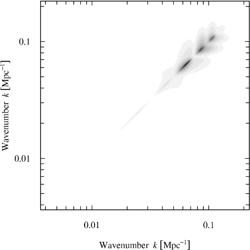
In Fig. 1 we illustrate the Fisher information matrix given by equation (2) which shows a band-diagonal structure with peaks of sensitivity to the primordial power spectrum on scales corresponding to the acoustic peaks; the sensitivity drops again on scales corresponding to the acoustic troughs, which can be remedied by information coming from the phase-shifted polarization peaks. Of course the sensitivity tends to zero on large scales due to a lack of modes to observe, and on small scales due to Silk damping and beam smoothing, since the $C_{\ell}$ of equation (2) is replaced by the total signal plus a Gaussian white noise model adjusted for a given experiment

$$C_{\ell}^{TT}\big{|}_{\rm noise} = \sigma_{{\rm noise}}^{2}e^{\ell(\ell+1)\theta^{2}/8\ln 2}\,,$$

$$C_{\ell}^{EE}\big{|}_{\rm noise} = 2\times\sigma_{{\rm noise}}^{2}e^{\ell(\ell+1)\theta^{2}/8\ln 2}\,,$$ (6)

$$C_{\ell}^{TE}\big{|}_{\rm noise} = 0,$$

where $\sigma_{{\rm noise}}^{2}$ is the noise variance in $(\mu$K-rad$)^{2}$ and $\theta$ is the FWHM of a Gaussian beam in radians. The noise model should be considered an important input to the analysis since it determines the range of scales that will be probed; it is an additional ingredient compared to the majority of analyses of the $C_{\ell}$ data. We use here a noise model for Planck with $\sigma_{{\rm noise}}^{2}=3\times 10^{-4}(\mu$K-rad$)^{2}$ and $\theta=7^{\prime}$, and a noise model for WMAP with $\sigma_{{\rm noise}}^{2}=8.4\times 10^{-3}(\mu$K-rad$)^{2}$ and $\theta=13^{\prime}$. In a realistic analysis the observed signal plus noise spectrum will be more appropriate.

Figure 2: Illustrating Planck’s window of sensitivity to the primordial power spectrum with and without polarisation (upper curve). Here $\sigma_{p}$ gives the approximate 1$\sigma$ error on measurements of the primordial power spectrum using bandpowers with $\delta\ln k\sim 0.02\rightarrow 0.05$. The vertical lines indicate the position of the temperature acoustic peaks. The cosmological parameters have been fixed, so some degrading of the sensitivity is expected.

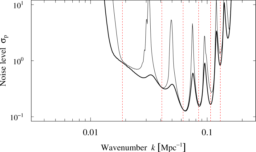
As usual the Fisher information matrix can be inverted to obtain a covariance matrix $C_{ij}$ whose diagonal components provide a useful estimate, the Cramer–Rao bound, of the expected variance of the parameters $p_{i}$ with

$$\sigma^{2}(p_{i})=C_{ii}\approx(F^{-1})_{ii}.$$ (7)

In Fig. 2 we plot this window of sensitivity to the primordial power spectrum (on a scale $\delta\ln k\sim 0.05$ set by the Fisher matrix bandwidth) for the Planck satellite, which can be seen to encompass the entire acoustic peak region. As noted in HO04, outside this range of scales, and in particular on large scales, we can only hope to recover wide-band ($\delta\ln k\gg 0.05$) averages of the primordial power spectrum at high accuracy.

The PCA basis $\{m_{i}\}$ is simply a linear combination of the power spectrum spike basis $\{p_{i}\}$

$$m_{a}=(\Delta\ln k)^{1/2}\sum_{i}S_{ia}p_{i}$$ (8)

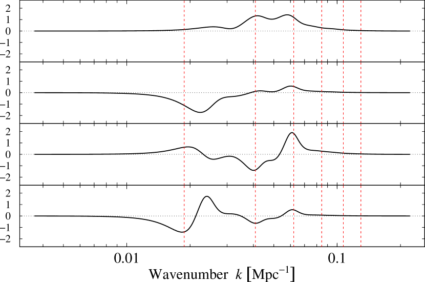
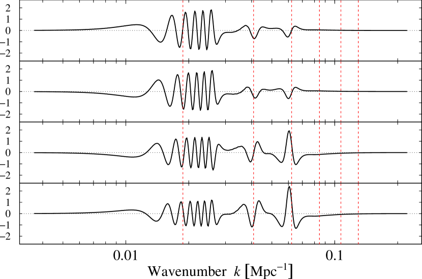
where the $S_{ia}$ are the orthonormal eigenvectors of the covariance matrix. We can then work with a set of normalised principal components ${\mathcal{S}}_{ia}=S_{ia}/\sqrt{\Delta\ln k}$ (hereafter the PCA modes) which will have unit variance when integrated over $\ln k$. In Figs. 3 and 4 we plot examples of the PCA modes with mode number from 1–4 and 17–20 respectively, generated using the WMAP noise model. The oscillations in the PCA modes become increasingly rapid at scales corresponding to the acoustic peaks where sensitivity to the primordial power spectrum is greatest, that is until we hit the numerical resolution. At this point the PCA modes branch into two wavepacket-like solutions travelling towards large and small scales, similar to the behaviour noted by Hamilton and Tegmark (2000), although this need not worry us. Note also that the PCA modes are invariant under changes in the discretisation scale $\Delta\ln k$. However, we found that in order to obtain sensible estimates of the eigenvalues (projected errors) of the PCA modes themselves, the Fisher matrix should be discretised on a scale that renders it roughly diagonal, instead of band-diagonal.

Figure 3: Illustrating PCA modes 1–4 which have been generated assuming the WMAP noise model. The vertical lines indicate the position of the temperature acoustic peaks.

The PCA modes can be straightforwardly integrated into the publicly available Markov Chain Monte Carlo (MCMC) package CosmoMC (Lewis & Bridle 2002, February 2005 version) in order to explore the full cosmological plus power spectrum posterior parameter space. Specifically, we use the following power spectrum ansatz

$$\frac{{\mathcal{P}}(k)}{{\mathcal{P}}_{0}}=m_{0}+\sum_{a=1}^{a_{{\rm max}}}m_{a}{\mathcal{S}}_{a}(k),$$ (9)

where we take ${\mathcal{P}}_{0}=23\times 10^{-10}$, which should be calibrated from observations. Clearly if the underlying primordial power spectrum is close to scale-invariant then equation (9) admits a solution

$$m_{a}=0,\,\,\forall a\Leftrightarrow\mbox{\rm Scale-invariance}.$$ (10)

More generally equation (9) is strongly suggestive of a general linear orthonormal model plus a noise term (see for instance Bretthorst 1988). In this way we are attempting to measure the spectrum of departures from scale-invariance which we call $\Delta{\mathcal{P}}/{\mathcal{P}_{0}}$ and which is given by the second term in equation (9); in this context the dominant scale-invariant component $m_{0}$ is a Gaussian noise term.

Concerning the numerical implementation of the power spectrum equation (9), we simply perform a linear spline in $\ln k$ over the discrete PCA modes ${\mathcal{S}}_{ia}$, which are added together before the final convolution with CMB transfer functions to obtain the $C_{{\ell}}$; outside the PCA mode $k$-range the second term of equation (9) is dropped. We checked that the default $k$-source and $k$-integration settings for CAMB modified to calculate $C_{{\ell}}$ at $\Delta\ell=3$ is accurate enough handle around the first forty modes of our current implementation; at this stage this is more than enough since we will only attempt to perform the MCMC with a maximum of sixteen PCA modes.

Figure 4: Illustrating PCA modes 17–20, as in Fig. 3. The oscillations are strongest in the vicinity of the acoustic peaks where the sensitivity to the primordial power spectrum is greatest.

Having obtained measurements of the PCA mode amplitudes from the MCMC, it is then straightforward to project any power spectrum model, for instance a power-law spectrum, onto the PCA modes via

$$m_{a} = \int d\ln k\,{\mathcal{S}}_{a}(k)\frac{\Delta{\mathcal{P}}}{{\mathcal{P}_{0}}}(k),$$ (11)

$$= \Delta\ln k\sum_{i}{\mathcal{S}}_{a}(k_{i})\left[\left(\frac{k_{i}}{k_{0}}\right)^{n_{{\rm S}}-1}-1\right],$$

in order to make the comparison with observations.

We can easily make an empirical estimate of the total signal to noise of the measured departures from scale-invariance

$$\frac{\rm S}{\rm N}=\left[\sum_{a=1}^{a_{{\rm max}}}\frac{\left<m_{a}\right>^{2}}{\sigma^{2}_{m_{a}}}\right]^{1/2},$$ (12)

where $\left<m_{a}\right>$ and $\sigma^{2}_{m_{a}}$ are the mean and variance of the individual mode amplitudes obtained from the MCMC. As noted by Kadota et al (2005), the PCA modes can be safely truncated as soon as ${\rm S}/{\rm N}$ saturates, assuming that the underlying primordial power spectrum is a reasonably smooth function. Incidentally, the total ${\rm S}/{\rm N}$ represents a useful figure of merit for optimising future CMB experiments to measure the primordial power spectrum sector. Other measures such as “risk” (Huterer & Starkman 2003) and Bayesian evidence (see for example MacKay 2003) could be used to provide a rationale for truncating the PCA mode amplitudes even further, given a power spectrum model of interest.

In the case that the recovered PCA mode amplitudes encode some complex information which can not be easily understood in the framework of power-law spectra, then it would be useful to obtain an estimate of $\Delta{\mathcal{P}}/{P_{0}}$ in $k$-space in order to aid the process of modelling the power spectrum. Here we use an estimator

$$\frac{\hat{\Delta{\mathcal{P}}}(k_{i})}{{\mathcal{P}}_{0}}=\sum_{a=1}^{a_{{\rm max}}}\left<m_{a}\right>{\mathcal{S}}_{a}(k_{i}),$$ (13)

and for the purposes of a comparison with the input spectrum, we estimate the noise variance via

$$\hat{\sigma}^{2}_{\frac{\Delta{\mathcal{P}}}{{\mathcal{P}}_{0}}}(k_{i})=C_{ii}+\sum_{a=1}^{a_{{\rm max}}}{\mathcal{S}}_{a}^{2}(k_{i})\sigma_{m_{a}}^{2},$$ (14)

where $C_{ii}$ is the covariance matrix, obtained from equation (7), accounting for the overall uncertainty in the narrow-band determination of ${\Delta{\mathcal{P}}}/{{\mathcal{P}}_{0}}$ in regions of lower sensitivity on large scales, small scales, and in the temperature acoustic trough regions.

A bandpower representation of the primordial power spectrum could also obtained from the measured PCA mode amplitudes via a Monte Carlo procedure; in this case the Fisher information matrix could be used for guidance when choosing the location and widths of the bands. Obviously though, no further quantitative information about the primordial power spectrum can be gleaned in this way.

Figure 5: Illustrating the recovery of the first eight mode amplitudes from simulated Planck data with an input scale-invariant spectrum. Plotted are the marginalised 1$\sigma$ error bars obtained from MCMC. The models (dashed lines) are for power-law spectra with $n_{{\rm S}}(k_{0}=0.05$ Mpc${}^{-1})=\{0.99,1,1.01\}$ (top to bottom, mode 1).

One final point worth making in this section concerns how one should deal with the inevitable degeneracies between the effect on the $C_{\ell}$ due to the cosmological parameters and the PCA power spectrum parameters, which will induce undesired off-diagonal components in the PCA covariance matrix. We sketch here the solution given in HO04: One must first form the joint Fisher information matrix, $F_{\mu\nu}$, for both power spectrum parameters and cosmological parameters

$$F_{\mu\nu}=\left[\begin{array}[]{rrr}F_{ij}&&B\\ B^{\rm T}&&F_{ab}\end{array}\right],$$ (17)

where $F_{ab}$ is the usual cosmological parameter Fisher information matrix (see for example Tegmark, Taylor and Heavens 1997) and $B$ are the cross terms. After inverting the full $F_{\mu\nu}$ to obtain a new covariance matrix $C_{\mu\nu}$, one simply retains the power spectrum parameter subblock $C_{ij}$, whose principal components will be “orthogonalized” to the effect of the cosmological parameters. In terms of implementation, one can use the matrix partitioning formulas (see for example Press et al 1992, Ó Ruanaidh & Fitzgerald 1996) to derive a “degraded” $F^{\rm deg}_{ij}$ subblock

$$F^{\rm deg}_{ij}=F_{ij}-B^{\rm T}F_{\rm ab}B.$$ (18)

We will make use of this in the next section.

Figure 6: Illustrating the estimated departures from scale-invariance in $k$-space on a narrow-band scale $\delta\ln k\sim 0.02$ for the case of an input scale-invariant spectrum. The solid curves show the estimated 1$\sigma$ error bars, given by equation (14). A scale-invariant spectrum within the acoustic peak region is strongly favoured.

3 Tests with Simulated Planck data

As a means of gaining experience with the PCA method we generate simulated Planck data up to an $\ell_{{\rm max}}=2250$ using the Gaussian white noise model of equation (2) for a cosmological model with parameters $\Omega_{{\rm B}}h^{2}=0.024$, $\Omega_{{\rm D}}h^{2}=0.121$, $H_{0}=72$, $\tau=0.17$, and ${\mathcal{P}}_{0}=2.3\times 10^{-9}$, which for simplicity are the same as those used to generate the PCA modes themselves. In a realistic data analysis scenario, the PCA modes would be generated with parameters close to the best-fit obtained from a traditional parameter determination approach. We consider three cases for the primordial power spectrum which is taken to described by a scale-invariant spectrum, a power-law spectrum with spectral index $n_{{\rm S}}=0.97$ and pivot scale $k_{0}=0.05\,{\rm Mpc}^{-1}$, and then finally a broken scale-invariance model with a Gaussian bump in the acoustic peak region

$$\frac{{\mathcal{P}}(k)}{{\mathcal{P}}_{0}}=1+0.1\exp\left[-\left(\frac{\ln\left[{k}/{0.08\,{\rm Mpc}^{-1}}\right]}{0.3}\right)^{2}\right].$$ (19)

We then perform MCMC over the full cosmological plus PCA mode parameter space using the simulated data up to an $\ell_{\rm max}=2000$. We have also varied the number of modes included in the analysis from zero to sixteen in steps of four in order to study the effect of truncating the PCA expansion on the recovery of the cosmological parameters.

The development of CosmoMC (Lewis & Bridle 2002) has reached a maturity that is very well suited to an analysis of this type where the number of power spectrum parameters begins to dominate over the number of cosmological parameters, but where we nonetheless expect by construction to obtain a stable multivariate Gaussian posterior solution. As a result we have taken full advantage of a conjugate gradients descent module which estimates the covariance and location of the posterior peak before the MCMC begins, thus alleviating the potential challenge working with so many parameters while also conserving some computing resources. On this note, the total number of $C_{\ell}$ likelihood evaluations required in our tests in the following section rises from around ${\mathcal{N}}_{\mathcal{L}}=2\times 10^{4}\rightarrow 10^{6}$ for zero and eight PCA modes respectively, and then tends to saturate at around this number. It seems reasonable that the number of likelihood evaluations ought not to exceed by much $\ell^{2}$, the total number of modes upon which the the $C_{\ell}$ spectrum depends. Moreover the ‘fast–slow’ split between power spectrum and cosmological parameter likelihood evaluation speeds, already implemented in CosmoMC, will be of increasing benefit as we attempt to measure up to perhaps thirty PCA mode amplitudes in the future (Kadota et al 2005).

3.1 The scale-invariant case

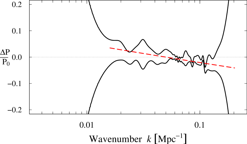
In Fig. 5 we illustrate the recovery of the first eight mode amplitudes for the $n_{{\rm S}}=1$ case and make comparison for the theoretical prediction for the mode amplitudes which are obtained by projecting some representative power-law spectra onto the PCA modes via equation (11); we find that the scale-invariant solution $m_{a}=0$ is very well recovered. Here it is worth mentioning that the Gaussian realisation for the simulated Planck data sets was taken to be the exact $C_{\ell}$ model, which explains why the recovery of the PCA mode amplitudes shows very little scatter around $m_{a}=0$. One can see that the first three PCA modes provide the bulk of constraining power for smooth power-law spectra leading to a constraint which will be roughly $n_{\rm S}=1\pm 0.01$, consistent with typical parameter forecasts in the literature.

Figure 7: Illustrating the recovery of the first ten principal component amplitudes from simulated Planck data with an input $n_{{\rm S}}=0.97$ spectrum, as in Fig. 5. The models (dashed lines) correspond to power-law spectra with $n_{{\rm S}}(k_{0}=0.05$ Mpc${}^{-1})=\{0.97,0.975\}$ (bottom to top, mode 3). The compressed CMB data can not be fit by $m_{\rm a}=0$ and so scale-invariance would be ruled out at high signal to noise.

We illustrate an estimate of the departures from scale-invariance $\hat{\Delta{\mathcal{P}}}/{\mathcal{P}}_{0}$ in Fig. 6, and the region with the most data weight can clearly be discerned showing consistency with a scale-invariant spectrum. In this case the recovery of the cosmological parameters is also excellent, and we recovered a stable Gaussian posterior (as a function of the number of PCA modes) with constraints given by $\omega_{\rm B}h^{2}=0.0240\pm 0.0002$, $\omega_{\rm D}h^{2}=0.121\pm 0.02$, $H_{0}=71.9\pm 0.7$, $\tau=0.170\pm 0.005$, ${\mathcal{P}}/{\mathcal{P}_{0}}=1.00\pm 0.01$ for the case of using eight PCA modes. Clearly the PCA method works well under these most idealised of circumstances.

3.2 The scale-free $n_{{\rm S}}=0.97$ case

Figure 8: Illustrating the estimated departures from scale-invariance in $k$-space for the case of an input $n_{{\rm S}}=0.97$ spectrum (inclined dashed line), as in Fig. 6. A tilt is recovered in the region $k=0.06-0.1$ Mpc^-1 with enough signal to noise to overrule the assumption of scale-invariance in model equation (9).

The $n_{{\rm S}}=0.97$ case is more delicate since we know in advance that the power spectrum model equation (9) will not be able to accurately describe a tilted spectrum on large or small scales. We can therefore expect some biasing in the recovery of the cosmological parameters which will necessarily adjust to provide the overall excess of power on large scales relative to small scales; this is just the usual degeneracy between cosmological and power spectrum parameters.

In fact to get reasonable results at all, we found it necessary to apply equation (18) in order to orthogonalise the PCA modes to the effect of the primordial power spectrum amplitude ${\mathcal{P}_{0}}$. The qualitative effect on the PCA modes is the the positive definite mode 1 is removed. Having modified the PCA modes in this way, the cosmological parameters are recovered as $\omega_{\rm B}h^{2}=0.0247\pm 0.0002$, $\omega_{\rm D}h^{2}=0.116\pm 0.001$, $H_{0}=74.6\pm 0.7$, $\tau=0.183\pm 0.006$, ${\mathcal{P}}/{\mathcal{P}_{0}}=1.02\pm 0.01$ for the case of using eight PCA modes, showing biases at the 3$\sigma$ to 4$\sigma$ level. The fact that the recovered dark matter density shifts from $\Omega_{{\rm D}}h^{2}=0.113\pm 0.001\rightarrow 0.116\pm 0.001$ as the number of PCA modes is increased provides a useful indication that there are problems afoot with our power spectrum model equation (9).

Interestingly however, the PCA mode amplitudes are still very well recovered, and we illustrate in Fig. 7 that the first ten mode amplitudes, if somewhat attenuated in amplitude, provide strong evidence for a power-law primordial power spectrum, showing a distinctive pattern deviating from scale-invariance, $m_{{\rm a}}=0$. The corresponding departures from scale-invariance are shown in Fig. 8 where the recovered power spectrum shows strong evidence for a tilt, modulo some attenuation and oscillations in regions of lower sensitivity. In short there is enough signal to noise to overrule our assumption of scale-invariance, supplying us with strong evidence that model of equation (9) needs refining. It is likely that in a more refined analysis, one should orthogonalise the PCA modes to the effect of the spectral index and the other cosmological parameters in order to recover unbiased estimates of the cosmological parameters.

3.3 The Gaussian bump case

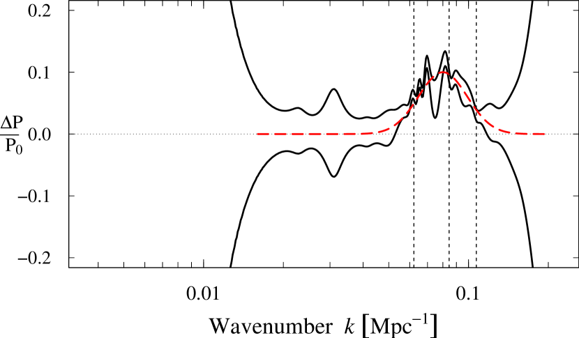
Although completely contrived, this is perhaps the most interesting and challenging case since the input primordial power spectrum now contains distinct feature within the acoustic peak region. We illustrate in Fig. 9 that the first sixteen PCA amplitudes are nonetheless rather well recovered and are consistent with the input Gaussian bump model. In this case we can see that, for instance, the second PCA mode strongly constrains the central position of the feature in $k$-space. In Fig. 10 we show that a bump like feature has indeed been recovered, again modulo some attenuation and oscillations in regions of lower sensitivity. The cosmological parameters are also very well recovered with $\omega_{\rm B}h^{2}=0.0238\pm 0.0002$, $\omega_{\rm D}h^{2}=0.122\pm 0.002$, $H_{0}=71.6\pm 0.9$, $\tau=0.170\pm 0.005$, ${\mathcal{P}}/{\mathcal{P}_{0}}=1.00\pm 0.01$. This represents an interesting success for the PCA method.

Figure 9: Illustrating the recovery of the first sixteen principal component amplitudes from simulated Planck data with an input Gaussian bump primordial power spectrum, as in Fig. 5. The models (dashed lines) correspond to the Gaussian bump of equation (19), centred on $k_{0}=\{0.082,0.08,0.078\}\,$Mpc^-1 (top to bottom, mode 2).

3.4 Summary and discussion

To summarise the tests so far, the PCA method has been demonstrated here to be very suitable and effective for measuring departures from scale-invariance, both scale-free and scale-dependent, in the most data-weighted regions of the $C_{\ell}$ spectrum. In a realistic data analysis setup the recovered PCA mode amplitudes, together with the PCA modes themselves will represent an extremely powerful compression of our information concerning the primordial power spectrum. At first sight this may represent an unnecessary data analysis stage compared the usual parameter determination methods where one fits to the $C_{\ell}$ data directly using the power spectrum model parameters on the same footing as the other cosmological parameters. However, the point here is to obtain first a detailed picture of the most important departures from scale-invariance in the primordial power spectrum while at the same time being able to weigh up the relative importance as well as locating both in $k$ and $\ell$ space any possible glitches or residual systematic effects in the $C_{\ell}$ data; then in the final data compression stage we can use the PCA mode amplitudes to rapidly test any wide class of specific power spectrum models with great ease and without recourse to any further $C_{\ell}$ likelihood evaluations, as was recently emphasised by Kadota et al (2005) for the case of inflation models.

4 Application to the WMAP data

In this Section we apply the PCA method to the currently available temperature and temperature-polarization cross correlation spectra from WMAP (Kogut et al 2003; Verde et al 2003; Hinshaw et al 2003) and bandpowers in the range $600<\ell<2000$ from the VSA (Grainge et al 2003; Dickinson et al 2004) ACBAR (Kuo et al 2004), CBI (Pearson et al 2003; Readhead et al 2004) and Boomerang B2K (Jones et al 2005, Piacentini et al 2005, Montroy et al 2005) instruments.

To emphasise once more, we are working within the framework of spatially flat $\Lambda$CDM cosmologies, described by five basic cosmological parameters: the baryon density $\Omega_{\rm B}h^{2}$, the cold dark matter density $\Omega_{\rm D}h^{2}$, the optical depth to last scattering $\tau$, the ratio of the sound horizon to angular diameter distance at last scattering $\theta=100r_{{\rm s}}^{*}/D_{{a}}^{*}$ (instead of $H_{0}$) and the overall amplitude of scalar perturbations ${\mathcal{P}}_{0}$. In addition we throw into the mix the first four PCA modes generated with a noise model for WMAP given by $\sigma_{{\rm noise}}^{2}=8.4\times 10^{-3}(\mu$K-rad$)^{2}$ and $\theta=13^{\prime}$.

Figure 10: Illustrating the estimated departures from scale-invariance in $k$-space for the case of an input scale-invariant plus Gaussian bump spectrum (dashed curve), as in Fig. 6. A distinct bump like feature is recovered in the acoustic peak region. Precision polarization data would be required in order to better recover the feature in between the third, fourth, and fifth temperature acoustic peak scales (vertical dotted lines).

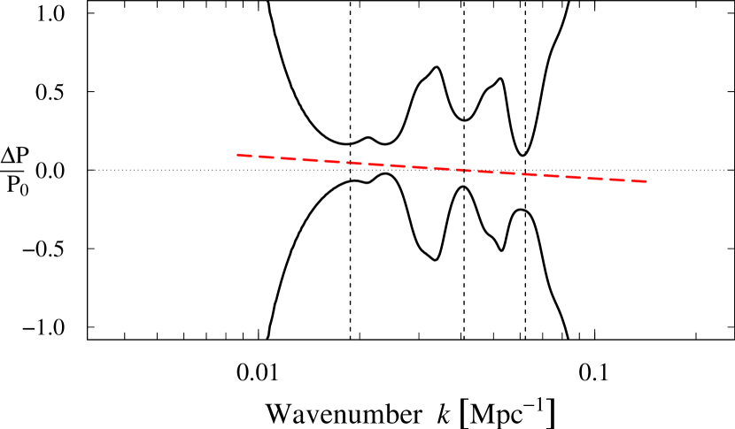
The measured amplitudes of the first four modes of Fig. 3 are displayed in Fig. 11 with the corresponding power spectrum in Fig. 12. The broad picture painted here is that we find no evidence for the breaking of scale-invariance: the mode amplitudes are very well fit my $m_{a}=0$. Only a single mode on scales corresponding to the second acoustic peak shows an S/N $>1$, which is barely worth mentioning aside from the fact that it can easily be accommodated by a slightly red primordial power spectrum: projecting power-law primordial power spectra onto the PCA basis and using a simple Gaussian likelihood function we find the constraint on the spectral index to be $n_{{\rm S}}(k_{0}=0.04$ Mpc${}^{-1})=0.94\pm 0.04$, displayed in Fig. 13, and which is in accordance with conventional studies of the primordial power spectrum. It is also possible to make a detailed comparison with the primordial power spectrum bandpowers from fig. 4 of Bridle et al (2003), as well as with orthogonal wavelet expansion constraints in fig. 2 of Mukherjee & Wang (2003b). We all find the same very weak trend for a 20-30$\%$ drop in power between between the first acoustic peak at $k=0.02$ Mpc^-1 and the third acoustic peak scale at $k=0.07$ Mpc^-1. Again, the trend is not so much interesting at this stage as the consistency between these complementary methods.

5 Conclusions

In this work we have implemented and investigated a principle component analysis (PCA) technique in order to study the possible departures from scale-invariance that may exist in the spectrum of primordial curvature perturbations, which are observable via the CMB anisotropies. The essence of this method is to decompose the primordial power spectrum into a scale-invariant component plus a series of orthonormal modes which reflect our expectation of where the departures from scale-invariance are likely to be best probed by the data. The information from the CMB is then be compressed into a series of mode amplitudes which can easily be compared with predictions from any wide class of primordial power spectra without recourse to any further $C_{\ell}$ likelihood evaluations.

Figure 11: Illustrating the current PCA measurements using current data from WMAP, VSA, ACBAR, CBI and Boomerang. The compressed CMB data are well fit by $m_{\rm a}=0$ and so show no evidence for breaking of scale-invariance. The dashed lines show power-law models with $n_{{\rm S}}(k_{0}=0.04$ Mpc${}^{-1})=\{1.0,0.94\}$ (top to bottom).

The method was first tested on simulated Planck data using an input scale-invariant spectrum and we observed good performance in the simultaneous recovery of cosmological parameters and the principal component mode amplitudes via an MCMC exploration of the full parameter space. In the case of simulated data from an input power-law spectrum with spectral index $n_{{\rm S}}=0.97$, the recovery of the cosmological parameters was biased as they adjusted to provide an overall excess of large-scale to small-scale power. However, the biasing is evidenced by fluctuating cosmological parameter constraints as the number of power spectrum principal components is increased. Moreover, the PCA mode amplitudes were still very well recovered, showing strong evidence for a tilted primordial power spectrum and providing enough signal to noise to overrule our assumption of scale-invariance. Thus PCA can be used as a self-consistent means for justifying a more refined power spectrum model than the one considered here in equation (9). We also demonstrated that the PCA method is capable of measuring departures from scale-free spectra by considering simulated data from a primordial power spectrum containing a $10\%$ gaussian bump in the acoustic peak region, and observing good recovery of both the PCA mode amplitudes and the cosmological parameters.

Figure 12: Illustrating the estimated departures from scale-invariance using current data from WMAP, VSA, ACBAR, CBI and Boomerang. The spectrum is scale-invariant showing only the slightest hint of a tilt. The best-fit spectrum with $n_{{\rm S}}(k_{0}=0.04$ Mpc${}^{-1})=0.94\pm 0.04$ is shown (dashed inclined line) as well as the first, second and third acoustic peak scales (vertical dotted lines).

Figure 13: Illustrating the posterior constraint on the spectral index $n_{{\rm S}}(k_{0}=0.04$ Mpc${}^{-1})=0.94\pm 0.04$ obtained from the four PCA mode amplitudes displayed in Fig. 11.

Finally, as a proof of concept of the method we provided a first glimpse of the principal component mode amplitudes that can be obtained from the currently available CMB data from WMAP, VSA, ACBAR, CBI and Boomerang. We obtained measurements of the first four principal components corresponding to scales across the first and second acoustic peaks, finding no evidence for the breaking of scale-invariance with only a hint of a red primordial power spectrum with spectral index $n_{{\rm S}}(k_{0}=0.04$ Mpc${}^{-1})=0.94\pm 0.04$, consistent with other studies in the literature, with a total signal to noise at not more than S/N $\sim 2.5$.

Assuming that the Gaussian adiabatic density perturbation scenario continues to hold as our observations of the CMB improve in the near future, then we will soon move into the regime where the information about the primordial power spectrum will completely outweigh the information about the cosmological parameters which become, from this perspective, well-understood nuisance parameters to be carefully integrated out. It seems very likely that principal component analysis, or else another very similar data compression technique, will be essential for fully exploiting the forthcoming temperature and polarization $C_{\ell}$ data.

References

- (1) Barger V., Lee H., Marfatia D., 2003, Phys. Lett. B, 565, 33
- Bennett et al. (2003) Bennett C. L. et al., 2003, ApJ. Suppl., 148, 1
- Bond et al (2004) Bond J. R. et al, 2004, Int. J. Theor. Phys., 43, 599
- (4) Bretthorst G. L., 1988, Bayesian Spectrum Analysis and Parameter Estimation, Springer-Verlag Berlin Heidelberg.
- Bridle et al (2003) Bridle S. L., Lewis A., Weller J., Efstathiou G., 2003, MNRAS, 342, L72
- (6) Dickinson C. et al, 2004, MNRAS, 353, 732-746
- (7) Dodelson S., 2003, Modern Cosmology, Academic Press
- (8) Grainge K. et al, 2003, MNRAS, 341, L23
- (9) Hannestad S., 2004, JCAP, 4, 02
- Hamilton & Tegmark (2000) Hamilton A. J. S., Tegmark M., 2000, MNRAS, 312 , 285-294
- Hinshaw et al. (2003) Hinshaw G. et al., 2003, ApJS., 148, 135
- Hu & Holder (2003) Hu W., Holder G.P., 2003, Phys. Rev. D, 68, 023001.
- Hu & Okamoto (2004) Hu W., Okamoto T., 2004, Phys. Rev. D, 69, 043004, (HO04)
- (14) Huterer D., Starkman G., 2003, Phys. Rev. Lett. 90, 031301
- (15) Jones W.C.. et al, 2005, ApJ submitted astro-ph/0507494
- Kadota et al (2005) Kadota K., Dodelson S., Hu W., Stewart E. D., 2005, 2005, Phys. Rev. D, 72, 023510
- (17) Kogut A. et al., 2003, ApJ Supp. 148, 161
- (18) Kuo C. L. et al., 2004, ApJ, 600, 32
- Kosowsky et al. (2002) Kosowsky A., Milosavljevic M., Jimenez R., 2002, Phys. Rev., D66, 063007
- (20) Leach S. M., Liddle A. R., 2003, Phys. Rev. D., 68, 123508
- Lewis & Bridle (2002) Lewis A., Bridle S. L., 2002, Phys. Rev., D66, 103511 (CosmoMC)
- (22) Lewis A., Challinor A., Lasenby A., 2000, ApJ, 538, 473 (CAMB)
- (23) Lewis A., Phys. Rev. D, 2005, 71, 083008
- (24) Liddle A. R., Lyth D. H., 2000, Cosmological Inflation and Large-Scale Structure, C.U.P.
- (25) Mackay D. J., 2003, Information theory, inference and learning algorithms, Cambridge University Press
- (26) Montroy T.E. et al, 2005, ApJ submitted astro-ph/0507514
- (27) Kogo N., Matsumiya M., Sasaki M., Yokoyama J., 2005, ApJ, 607, 32
- Mukherjee & Wang (2003) Mukherjee P., Wang Y., 2003a, ApJ, 593, 38
- Mukherjee & Wang (2003) Mukherjee P., Wang Y., 2003b, ApJ, 598, 779
- Mukherjee & Wang (2003) Mukherjee P., Wang Y., 2003c, ApJ, 599, 1
- Mukherjee & Wang (2005) Mukherjee P., Wang Y., 2005, JCAP, 0512, 007.
- (32) Pearson T. J. et al., 2003, ApJ, 591, 556
- (33) Peiris H. V. et al, 2003, ApJ, 148, 213
- (34) Piacentini F. et al, 2005, ApJ submitted astro-ph/0507507
- (35) Press W. H. Teukolsky S. A., Vetterling W. T., Flannery B. P., 1992, Numerical Recipes, Cambridge University Press.
- (36) R Development Core Team, 2004, R: A language and environment for statistical computing, R Foundation for Statistical Computing, URL http://www.R-project.org
- (37) Readhead A. C. S. et al., 2004 ApJ, 609, 498
- (38) Ó Ruanaidh J.J.K and Fitzgerald W.J. 1996, Numerical Bayesian Methods Applied to Signal Processing, Springer-Verlag, New York.
- (39) Seljak U., Zaldarriaga M., 1996, ApJ, 469, 437
- (40) Seljak U., Sugiyama N., White M., Zaldarriaga M., 2003, Phys. Rev., D, 68, 083507
- (41) Shafieloo A., Souradeep T., 2004, Phys. Rev., D70, 43523
- (42) Tochini-Valentini D., Douspis M., Silk J., 2005, MNRAS, 359, 31
- tegmark et al (1997) Tegmark M., Taylor A. and Heavens A., 1997, ApJ, 480, 22-35
- (44) Tegmark M., Zaldarriaga M., 2002, Phys. Rev. D, 66, 103508
- Verde et al. (2003) Verde L. et al., 2003, ApJ Suppl., 148, 195
- (46) Wang Y., Spergel D., Strauss M. A., 1999, ApJ, 510,20
- Zel’dovich & Novikov (1975) Zel’dovich Ya. B., Novikov I. D., 1975, Vol. 2: Structure and Evolution of the Universe, Moscow, Izdatel’stvo Nauka.