Radiative transfer in moving media

A new method for the formal solution of the 2D radiative transfer equation in axial symmetry in the presence of arbitrary velocity fields is presented. The combination of long and short characteristics methods is used to solve the radiative transfer equation. We include the velocity field in detail using the Local Lorentz Transformation. This allows us to obtain a significantly better description of the photospheric region, where the gradient of the global velocity is too small for the Sobolev approximation to be valid. Sample test calculations for the case of a stellar wind and a rotating atmosphere are presented.

1 Introduction

Radiation is the major source of information about stars. A number of stellar properties can be obtained by comparing observed spectra with the synthetic ones calculated from model stellar atmospheres. A key problem in computing synthetic spectra is solving the radiative transfer equation in stellar atmospheres, since the emergent radiation is formed in these regions. There exists a large number of methods for solving the transfer equation in a static one-dimensional case, which are, unfortunately, inappropriate for stars with stellar winds, rapidly rotating stars, accretion discs, and also for nebulae. Our main interest is to study various aspects of the stellar wind in hot stars, therefore we want to develop a method for solving the radiative transfer equation that is well suited for this case, where the symmetries enabling a one-dimensional approximation are broken.

There are not many methods available to solve static multidimensional radiative transfer problems. For optically thin regions, the Monte Carlo method (Boissé boisse (1990)) may be used. On the other hand, in the optically thick regions it is possible to solve the transfer equation using a method that employs the diffusion approximation (Kneer & Heasley difuzemulti (1979)). Neither of these methods are suitable for stellar atmospheres, where the transfer problem must be solved from optically thick regions to regions where the optical thickness is very small. The classical way of solving the radiative transfer equation in more dimensions is the long characteristics method (Cannon dlouhy (1970)). This method fully describes the radiation field, but the computer time necessary to obtain a solution may become long. For this reason, Kunasz & Auer (kratky (1988)) developed the short characteristics method, which is the best currently available multidimensional method. There exist several applications of short characteristics methods in a Cartesian grid (Fabiani Bendicho (zaklad, 2003, and references therein)) and 2D axially symmetric geometry (Georgiev et. al bulhar (2003)). Dullemond & Turolla (dullemond (2000)) developed a “rotating plane” method for axially symmetric problems based on the short characteristics method, too. An efficient approach is to use adaptive grids following Folini et al. (doris (2003)) and Steinacker et al. (steinray (2003)). A review by Auer (2003b ) provides an excellent insight into the grounds for astrophysical multidimensional radiative transfer.

Another possibility is to apply the finite element method, which has been recently used for multidimensional radiative transfer by, e.g., Richling et al. (femulti (2001)). However, the finite element method is not used very often for radiative transfer in stellar atmosphere studies due to its convergence problems caused by the about ten orders of magnitude changes of physical quantities (e.g. opacity, density) in stellar atmospheres. Dykema et al. (DFEIII (1996)) tried to overcome the instability and convergence problems using a modification of the finite element method, namely, the discontinuous finite element method. The discontinuous finite element method was also used in our previous paper (Korčáková & Kubát kk (2003), hereafter Paper I) for one-dimensional radiative transfer.

If the velocity field is present, the situation is more complicated. The changes in opacity and emissivity along a ray in spectral lines can be large due to the Doppler shift, and we have to take this into consideration. In the continuum, we can simply use the static equation, since the Doppler shift has only a small effect on the opacity and emissivity coefficients. For simplicity the methods assuming monotonic velocity field have been used very often. The multidimensional problem with velocity fields can be solved in the observer frame (the frame connected with the center of a star) or in the comoving frame (the frame connected with the outflowing material). Radiative transfer in more dimensions has usually been solved in the observer frame (e.g. Carlsson & Stein multitubingen (2003)). One of the firsts works to do this is Mihalas, Auer & Mihalas (mihalas78 (1978)), who were able to solve a periodic velocity field in two-dimensional planar geometry. Recently, van Noort et al. (vnapj (2002, 2003)) solved this problem in two dimensions. Their code is able to cope with both spherical and cylindrical geometry for Cartesian coordinate systems. The observer frame is appropriate only for small velocity gradients. The velocity difference between neighbouring depth points has to be smaller than several times the thermal velocity. If the velocity gradient is large, the Sobolev approximation (Sobolev Sobolev (1947)) is often used. This approximation was used for a 3D case by Folini et al. (doris (2003)). Both cases of small and large velocity gradients can be solved in the comoving frame. For a 3D accretion disc, the radiative transfer in the comoving frame was solved by Papkalla (papkalla (1995)).

However, there exists another effect that is usually neglected or taken into account in an approximate manner, namely the rotation of stars. Stellar rotation is usually taken into account as a convolution of the line profile, obtained from the plane-parallel static solution, and of the rotation profile (cf. Gray konvoluce (1976)). In this technique one must make use of analytical expressions for limb darkening, which do not give a correct description of the angular dependence of the specific intensity. It also does not take into account the fact that limb darkening is strongly frequency dependent across the line profile (cf. Hadrava & Kubát hadku (2003)). In order to describe the radiation field and its influence on the stellar atmosphere correctly, it is also necessary to take into account the Doppler shift of lines in a rotating atmosphere for the transfer of radiation along nonradial rays.

In this paper we present a new method to formally solve the radiative transfer equation in axial symmetry, which does not employ the Sobolev approximation. Our method is based on the Local Lorentz Transformation method (LLT) described in Paper I for the one-dimensional case. For studies of stellar wind, accretion discs or stellar rotation we need a method that uses a more general geometry than plane-parallel or spherical. However, it is not necessary to treat the whole three dimensional space in detail. We employ axial symmetry. The results will be more accurate than in a plane-parallel or spherical geometry and the calculation will be faster than for the full 3D problem.

In the first part of this paper we present our axially symmetrical code. The geometry of the model is described in detail, followed by some tests of our code. We compare these results with a spherically symmetric model atmosphere from Kubát (ATAmod (2003)). We also present some test calculations with a velocity field. Our line profiles are compared with convolved profiles for the case of stellar rotation. Some results for the stellar wind are also shown. Then we test the dependence of the computing time on the number of grid points. In the last part, we comment on the possibilities of the application for our method.

2 Method

We solve the radiative transfer equation for the specific intensity of radiation $I$

$$\@vec{n}\cdot\nabla I\left(\@vec{r},\@vec{n},\nu\right)=-\chi\left(\@vec{r},\nu\right)\left[I\left(\@vec{r},\@vec{n},\nu\right)-S\left(\@vec{r},\nu\right)\right],$$ (1)

where $\chi$ is the opacity, $S$ is the source function, $\@vec{n}$ is the direction of radiation, $\@vec{r}$ is the radius vector, and $\nu$ denotes the frequency. We assume axial symmetry and we allow for a nonzero velocity field.

The basic idea of this method is to solve the radiative transfer problem not in the whole star, but in separated planes intersecting the star.

2.1 The spatial grid

Let us consider the spherical coordinate system ($r$, $\theta$, $\phi$). We choose as the axis of symmetry $\theta=0$ (see Fig. 1). First, we introduce the discretization of the radial distance $r$ and angle $\theta$. Due to the axial symmetry, physical quantities do not depend on the angle $\phi$. The grid is chosen to give the best description of the system, depending on the studied object. As an example, for the study of stellar winds, the grid of angles $\theta$ can be equidistant. On the other hand, for accretion discs it must be finer near the equatorial plane, where the disc resides. In radial distance $r$ we choose the grid (very similarly to a 1D problem) to be equidistant in the logarithm of the radial optical depth. A suitable choice is about 5 points per decade. We assume the opacity and emissivity of the stellar material to be known at the grid points.

To reduce the 3D problem to a 2D one, we do not solve the radiative transfer equation directly in the 3D grid, but in a set of “longitudinal planes” intersecting the star parallel to the plane $\phi=0$ (we “slice the star” – see Fig. 1). In thin stellar atmospheres it is favourable to choose a finer grid of longitudinal planes closer to stellar limb, since the limb darkening is better described by such a choice.

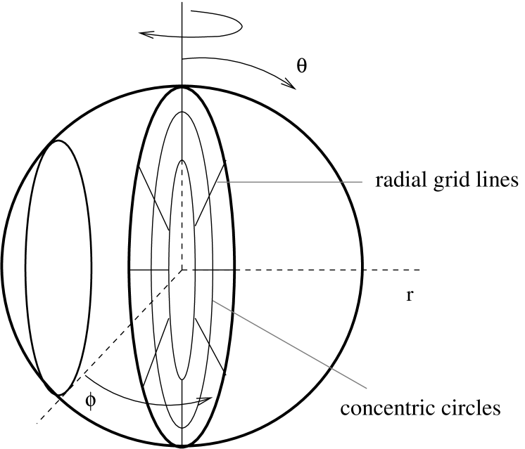
Figure 1: Coordinate system and the set of longitudinal planes. These planes are parallel to the plane $\phi=0$. Note that some of them intersect the opaque stellar core, where the diffusion approximation is valid, while the rest does not.

The primary grid described above helps us only to interpolate the quantities to the selected planes and finally to calculate the emergent flux. To solve the transfer equation we need a slightly modified grid. For each longitudinal plane we choose the polar coordinate system and define a grid of concentric grid circles and radial grid lines (see Fig. 1). The grid of concentric circles corresponds to the original 3D grid in the planes, which intersect the opaque stellar core where we do not solve the transfer equation and where we apply the lower boundary condition following from the diffusion approximation. However, choosing an appropriate grid for planes which do not intersect the opaque stellar core may become difficult, since the grid chosen must correspond to the geometry of the problem as well as resolving the velocity field. This is shown in Fig. 2. We must provide an appropriate grid

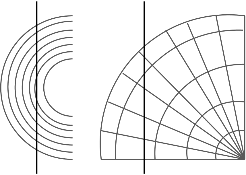
Figure 2: Choosing the grid in longitudinal planes that do not intersect the opaque stellar core. For geometrically thin (left panel) atmospheres, the grid points are defined using intersections of a longitudinal plane with concentric circles. For extended atmospheres (right panel), intersections of the longitudinal plane with radial lines are used for the definition of grid points.

for both geometrically thin and extended atmospheres.

For geometrically thin atmospheres the grid of radial distances in the longitudinal plane is chosen using intersection points with grid circles in the primary 3D grid (left panel in Fig. 2). For an extended atmosphere it is better to define grid points where the plane intersects the radial grid lines (right panel in Fig. 2). The reason why we need an appropriate grid in the planes that do not intersect the inner boundary is the necessity to ensure sufficient spatial resolution for the radiative transfer equation solution. This may be difficult in the central region of the plane. Moreover, similar problem involves by the velocity field. The velocity gradient in the planes far from the center can be large, so it is necessary to have a sufficient number of grid points.

The opacity, emissivity and the source function are interpolated to the new coordinate system. Linear interpolation is used here, since the grid is not orthogonal. The radiative transfer equation is solved for each longitudinal plane independently (Section 2.3). The whole radiative field is obtained by rotating the separate planes around the axis of symmetry (Section 2.4).

2.2 The frequency grid

The frequency grid is to be chosen to enable the most efficient description of the radiation field. We set the frequency interval using both the largest line width and the total Doppler shift caused by the global motion. For example, for Doppler profile this interval is

$$\nu\in\langle \nu_{0}\left(1-(\text{v}_{\infty}+\text{v}_{rot_{0}})/c\right)-2\Delta\nu_{D},$$

$$\nu_{0}\left(1+(\text{v}_{\infty}+\text{v}_{rot_{0}})/c\right)+2\Delta\nu_{D}\rangle,$$ (2)

where $\text{v}_{\infty}$ is the terminal velocity, $\text{v}_{rot_{0}}$ the rotation velocity in photosphere. $\Delta\nu_{D}$ denotes the broadest Doppler halfwidth, which corresponds to the highest temperature. For very extended atmospheres or planetary nebulae (optically thin medium) we must take into account that the regions with $-\text{v}_{\infty}$ and $\text{v}_{\infty}$ “see” each other. In that case, we must multiply $\text{v}_{\infty}$ in Eq. (2) by two. We take the frequency step to be equidistant for the case of the Doppler line profile. This step must be small enough to describe the line profile variations in the region with low temperature. The step is determined in the following way. We first typically set 5 points per line equidistantly at the depth point with the narrowest line profile (which is usually the depth point with the lowest temperature). Then we cover the whole frequency interval (2) with frequency points using this frequency step. This frequency grid is then used in other depth points where the line profile is broader. For a Voigt profile we need to extend the frequency interval (2), but the frequency step in the extended part of the interval may be larger.

2.3 Solution in longitudinal planes

In the given longitudinal plane we introduce the polar coordinate system using grid circles and radial grid lines defined in the preceding subsection (2.1). The values of temperature, density and velocity are known at the grid points. First, we solve the transfer equation in the plane starting at the outer boundary. Once the radiation field in the direction towards the center is known, we can continue to solve the transfer equation in the opposite direction, i.e. from the inner boundary towards the outer one. At the inner boundary the diffusion approximation may be taken for planes intersecting the opaque stellar center as a boundary condition. In other planes (that do not intersect the stellar center), we adopt as the lower boundary condition the intensity taken from the previously calculated solution from the outer boundary inwards.

2.3.1 The solution from the outer boundary to the central regions

We begin the calculations at the outer boundary (stellar surface), where the boundary condition (i.e. the incoming intensity $I$) is known. At each inner grid point we choose several rays per quadrant (see Fig. 3). The rays start at the outer grid circle and end at a given grid point.

Figure 3: Diagram for the solution of the radiative transfer equation in the longitudinal plane starting at the upper boundary to the central regions. The rays along which we perform the formal solution are plotted using the dashed line.

Along these rays we solve the transfer equation. The angle distribution of these rays may be the same as often used in the case of the plane-parallel geometry, where the angle cosines $\mu=\cos\alpha$ ($\alpha$ is the angle between the ray and the radial direction, see Fig. 3) are chosen to be the roots of Legendre polynomials in the interval $(0,1)$ ($\mu=0.8872983346$, $0.5$, $0.1127016654$) to ensure better numerical accuracy of the angle integration (Press et. al (recipes, 1986, section 4.5)). Three rays at a given point is usually sufficient, because the whole radiation field is obtained by summing the information from all longitudinal planes intersecting the given point (see Fig. 7). However, in some situations it is better to use more (up to 9) rays per quadrant to overcome a numerical error introduced by the necessary interpolation of intensity described below. As one can see in Fig. 3, the rays start at the preceding grid circle. This means that the rays do not usually start at a grid point and that they may also intersect some radial grid lines.

The solution diagram is illustrated in Fig. 4. We perform a linear interpolation of the source function and opacity to obtain their values at points $A$, $B$, and $C$ and of the incoming intensity for the value at point $A$.

Figure 4: The scheme for the integration along the ray for a determination of the specific intensity at the point $D$. The specific intensity at the grid points of outer grid circle is known. The value of the specific intensity at the point $A$ is determined by linear interpolation from values at neighbouring grid points. The values of the source function and opacity in the points $B$ and $C$ are obtained by linear interpolation.

The optical depth difference $\Delta\tau$ is calculated along the ray between the individual intersection points (abscissas $AB$, $BC$, and $CD$) using the linear approximation,

$$\Delta\tau_{(AB)}=\frac{\chi_{A}+\chi_{B}}{2}\Delta s_{(AB)},$$ (3)

and similarly for $\Delta\tau_{(BC)}$ and $\Delta\tau_{(CD)}$. Here $\chi_{A}$ and $\chi_{B}$ are opacities at respective points and $\Delta s_{(AB)}$ is the geometrical distance between points $A$ and $B$.

We solve the equation of radiative transfer by parts between all intersection points along the ray. We assume a linear dependence of the source function on the optical depth between the intersection points. For the interval $AB$ the solution is

$$I_{(B)}=I_{(A)}e^{-\Delta\tau_{(AB)}}+\int^{\Delta\tau_{(AB)}}_{0}S(t)e^{[-(\Delta\tau_{(AB)}-t)]}dt,$$ (4)

and similarly for intervals $BC$ and $CD$. The final intensity $I_{(D)}$ at the grid point $D$ is thus determined by three successive applications of the equation (4). In this manner we obtain the specific intensity in the downward solution at every grid point. It may, of course, happen that the geometric distance along the ray in the given cell is very small (the ray near the point $B$ in the Fig. 4). In this case we do not solve the transfer problem in this cell and we simply set $I_{(B)}=I_{(A)}$. Doing this, we eliminate a numerical instability. Usually, it is enough if the condition $|\cos(\pi/2-\theta-\alpha)|>10^{-7}$ ($\alpha$ has the same meaning as in Fig. 3) is fulfilled, even if it is much more accurate to estimate it using the optical depth difference.

There are several reasons why we prefer only a linear dependence of the source function on other higher order approximations. First, it is numerically stable and second, it is much faster. The higher order optical depth interpolation may sometimes lead to numerical errors by adding new extrema (cf. Auer 2003a ). They may become significant especially in moving medium. There is only one reason why linear interpolation should not be used: because the diffusion approximation in deep optically thick layers would be inaccurate. Since we do not solve the transfer problem using the short characteristics method, this inaccuracy is not large in our case. Our characteristics are longer and the transfer equation is solved in several steps, so the information from the farther regions is naturally included. Therefore we chose the safer linear interpolation.

2.3.2 The solution from the central regions to the outer boundary

The upward solution is very similar to the previous step. The procedure is depicted in Fig. 5. We lead the rays to the grid points

Figure 5: Diagram for the solution of the radiative transfer equation from the center of the star to the outer boundary. The rays along which we solve the formal solution are plotted using the dashed line.

using the same angles as in the previous case. The rays start either at the preceding grid circle (closer to the center) or at the same circle as the grid point. At the intersection points we interpolate the opacity and the source function. Between these points we calculate the optical depth using (3) and solve the transfer equation using (4) as in the previous case of downward integration.

From Fig. 1, one can see that there exist planes that do not intersect the inner boundary region. For these planes we adopt the intensity calculated from the previous step (solution from the upper boundary to the stellar center) as the lower boundary condition. However, the solution of the transfer equation in the central grid circle must be performed with care. The situation is shown in the Fig. 6. First, we solve the radiative transfer equation from the intersection point $A$ to the center of the abscissa $AC$ (point $B$) and then to point $C$. The physical quantities at point $B$ we obtain by linear interpolation from points $A$ and $C$. The optical depth difference is calculated using (3) and the specific intensity is determined using (4). The value of the intensity at point $C$ determines the lower boundary condition for further solutions outwards.

Figure 6: Diagram for a solution of the radiative transfer equation in the central region in the planes, which do not intersect the region of validity of the diffusion lower boundary condition.

For planes, which intersect the region of validity of the diffusion approximation (the stellar core), the situation is easier. We simply use the appropriate lower boundary condition.

2.4 The full radiation field

To obtain the whole radiation field we take the advantage of the symmetry of the problem. We know the radiation field at grid points in all directions lying inside the longitudinal planes. The radiation field in the whole star is then obtained by rotating the longitudinal planes around the axis of symmetry $\theta=0$ (see Fig. 7). This gives a sufficient description of the specific intensity.

Figure 7: Diagram describing the determination of the whole radiation field. The rotation axis for longitudinal planes is perpendicular to the page. Longitudinal planes (projected as lines in this figure) are rotated along the axis to intersect at a point $R$. Due to the axial symmetry, the radiation field for all directions is obtained by a rotation of all longitudinal planes around the axis of symmetry.

The emergent radiation flux towards the observer is calculated by integrating specific emergent intensity over the stellar disc.

2.5 Velocity field

The radiative transfer equation in moving media can be solved either in the observer frame or in the comoving frame. Since the coefficients of emissivity and opacity are angle dependent in the observer frame, we solve this problem rather in the comoving frame. This frame, which is coupled with the moving medium, is generally a non-inertial frame. The form of the radiative transfer equation in the comoving frame we can obtain either from the general relativity or from the special relativity by assuming a set of Local Lorentz Transformations.

In the Paper I we introduced an LLT (Local Lorentz Transformation) method for a solution of the radiative transfer equation in one-dimensional moving media based on an application of Lorentz transformations on cell boundaries and a static radiative transfer equation solution between them. The method was tested by a comparison with an exact solution of the radiative transfer equation using the discontinuous finite element method (see Fig. 8 in Paper I), which solves the comoving transfer equation including the $\partial/\partial\nu$ (Doppler) and $\partial/\partial\mu$ (aberration) terms. Here we apply the same idea for the case of a two-dimensional arbitrarily moving medium.

In our method, we replace the solution of the radiative transfer equation in the comoving frame by a set of Local Lorentz Transformations and a solution of the transfer equation in corresponding local inertial frames. In these inertial frames we solve a static radiative transfer equation, since it is Lorentz invariant. To do this, we must consider the constant velocity of every cell and the change of the velocity we allow only at the cell boundary (see Fig. 8).

Figure 8: The scheme for the inclusion of the velocity field. Velocity within each cell is constant and a change of velocity is possible only at the cell boundaries.

Two other conditions must be fulfilled there. First, velocity with respect to the observer frame must be low to neglect aberration. This permits us to solve the radiative transfer along straight characteristic lines. This assumption is valid, if $\text{v}/c\ll 0.01$ (Mihalas et al. CMF3 (1976), Hauschildt et al. H95 (1995)). Second, let us assume a steady-state fluid. Due to this assumption we can neglect the time delay between different parts of the medium. The correctness of this approach has been discussed in more detail in Paper I, where this method was tested for a plane-parallel geometry.

The basic solution scheme within cells, which was described in Section 2.3, is not affected by the presence of the velocity field. We project the velocity field to the longitudinal planes. At cell boundaries we perform the Lorentz transformation of frequency $\nu$ (see also Eq. (24) in paper I)

$$\nu^{\prime}=\nu\sqrt{1-\frac{\left(\Delta\text{v}\right)^{2}}{c^{2}}}\left(1-\frac{\@vec{n}\cdot\Delta\@vec{\textbf{v}}}{c}\right)$$ (5)

($\Delta\@vec{\textbf{v}}$ is the velocity difference between cells). Since the velocity field is not relativistic, we can simply use the classical Doppler law, which speeds up the solution. The Lorentz transformation of intensity $I^{\prime}\left(\nu^{\prime}\right)=I\left(\nu\right)\left({\nu^{\prime 3}}/{\nu^{3}}\right)$ (see Eq, (23) in Paper I) at the cell boundary has a negligible effect, and we do not take it into account, since the intensity is proportional to the third power of the frequency ratio. This is close to one in most stellar applications. Since the equation of the radiative transfer is Lorentz invariant, we solve the static equation of the radiative transfer (4) within each cell.

Since we solve the transfer equation in the comoving frame, we have to do one additional step. We know the source function and opacity in the frequency grid points in the rest frame coupled with a given cell. The incoming intensity from a neighbouring cell is known at different frequencies, which are Doppler shifted according to the velocity difference between the cells. This means that we must interpolate the intensity to frequency points coupled to the rest frame of a cell.

To ensure a correct treatment of line transfer we have to guarantee that the frequency shift at the cell boundaries due to Doppler effect is smaller than a quarter of a Doppler halfwidth (see Paper I). If it is not, we must make the grid finer. This condition must be fulfilled even if we calculate with the Voigt profile since the center of the line has a Doppler core. This is the only limitation of this method. If the velocity gradient is too high, we must refine the grid, which slows down the calculation.

3 Test calculations

Tests of the method are based on a model atmosphere of a main sequence B star with effective temperature $T_{\mathrm{eff}}=17\times 10^{3}\ \mathrm{K}$, gravitation acceleration $\log g=4.12$, and radius $3.26R_{\odot}$. We obtain the state parameters, electron density and temperature, using the hydrostatic spherically symmetric model atmosphere code ATA (Kubát ATAmod (2003)). We consider no incoming radiation as the outer boundary condition and the diffusion approximation as a lower boundary condition.

3.1 Static case

For a basic comparison we took a model atmosphere calculated using the static computer code ATA. The radiative transfer in ATA is solved using the long characteristics method and Feautrier variables (see Kubát ATAdis (1993, 1994, 2003)). We compare the result from the ATA code with the flux obtained from our new code (Fig. 9). The line profile was chosen to be Doppler here and the input parameters in the axially symmetric code are independent of $\theta$. This comparison for this simplest case proves the basic correctness of the new code.

Figure 9: The comparison of Eddington flux in the ${\mathrm{H}}\alpha$ line from the static spherically symmetric code ATA (crosses) and the axially symmetric one (solid line).

3.1.1 Limb darkening

An important result arising from the solution of the transfer equation is the limb darkening law. In Fig. 10 we plotted the limb darkening law across the ${\mathrm{H}}\alpha$ line profile calculated from our code. We choose as an x-axis the distance from the center of star in star radius units ($x=1$ for $r=R_{\star}$, where $R_{\star}$ is the stellar radius). At this scale the effect of limb darkening is more clearly visible.

Figure 10: Theoretical limb darkening obtained using our code across a half of the stellar disk in the ${\mathrm{H}}\alpha$ line. $R_{\star}$ denotes the stellar radius.

To show this effect in more detail, we extracted the dependence of the specific intensity on the distance from the center of the stellar disc for a continuum frequency (Fig. 11) and for the central frequency of the ${\mathrm{H}}\alpha$ line (Fig. 12).

Figure 11: Limb darkening in the continuum. Crosses denote data computed from our model. The fitting functions $f(x)$ and $g(x)$ which express the commonly used limb darkening laws are defined by equations (6) and (7).

The obtained data for the continuum are compared with functions usually used to express the limb darkening law. The first function ($f(x)$) is adopted from Allen’s Astrophysical Quantities (allen (1963)),

$$I(x)=1-a-b+a(1-x^{2})^{1/2}+b(1-x^{2})\equiv f(x).$$ (6)

Using the least squares method we obtain the parameters $a=0.55\pm 0.02$ and $b=-0.20\pm 0.01$ to fit our results to Eq. (6). Limb darkening is also often described by the law (Gray konvoluce (1976)),

$$I(x)=(1-\epsilon)+\epsilon(1-x^{2})^{1/2}\equiv g(x).$$ (7)

Fitting this case we obtain the value of the parameter $\epsilon=0.277\pm 0.008$.

Figure 12 shows the limb darkening in the center of the ${\mathrm{H}}\alpha$ line.

Figure 12: Center-to-limb variations at the central frequency of the ${\mathrm{H}}\alpha$ line. Note the apparent weak limb brightening before final darkening at the stellar limb.

As one can see, brightening instead of darkening is observed near the stellar limb, which corresponds to the effect of flash spectra in solar chromosphere. The same result was obtained also by Hadrava and Kubát (hadku (2003)).

3.2 Stellar wind

The case of the moving atmosphere is first tested for a spherically symmetric stellar wind, for which we adopt the beta law for the dependence of the wind velocity v on radius $r$ (see, e.g., Lamers & Cassinelli CL99 (1999))

$$\text{v}(r)=\text{v}_{\infty}\left\{1-\left[1-\left(\frac{\text{v}_{R}}{\text{v}_{\infty}}\right)^{\frac{1}{\beta}}\right]\frac{R}{r}\right\}^{\beta}.$$ (8)

We choose a velocity in the photosphere of $\text{v}_{R}=200\,\mathrm{km}\leavevmode\nobreak\ \cdot\leavevmode\nobreak\ \mathrm{s}^{-1}$ and a terminal velocity $\text{v}_{\infty}=2000\,\mathrm{km}\leavevmode\nobreak\ \cdot\leavevmode\nobreak\ \mathrm{s}^{-1}$.

To check the consistency of our new method we compare it with the plane-parallel method described in Paper I. The plane-parallel radiative transfer equation is solved using the discontinuous finite element method. The velocity field is included using the Local Lorentz Transformation similarly to this paper. In Paper I the Local Lorentz Transformation method was compared with the solution of the radiative transfer equation using the discontinuous finite element method, where the frequency term was consistently included into the solution as an independent variable. Since the velocity field is non-relativistic, calculations with aberration give the same results as without it (in agreement with Mihalas et al. CMF3 (1976), Hauschildt et al. H95 (1995)).

Figure 13: The comparison of the ${\mathrm{H}}\alpha$ line profile obtained from our axially symmetric model (solid line) and a plane-parallel model (denoted by 1D LLT). The dotted line is obtained using the same model, but the radiation with $\mu<0.26$ is not taken into account to approximate the curvature of the atmospheric layers (see also Fig. 14). The beta velocity law parameter $\beta=1$ for all profiles.

The result from plane-parallel geometry is plotted using the dashed line in Fig. 13. As we can see, the agreement with the new (axially symmetric – solid line) results is not good. The reason is in the geometry used. Rays with large angle (low $\mu$) in a curved atmosphere (spherically symmetric or axially symmetric) do not even touch regions that are optically thick in continuum, whereas for a plane parallel geometry all rays with $\mu>0$ finally reach the continuum optically thick regions (see Fig. 14). As a consequence, there is more continuum radiation in a plane parallel geometry, which results in shallower line profiles. This has been well known for a long time (see, e.g., Kunasz et al. spher2 (1975)).

Figure 14: Intensity obtained from plane-parallel and axially symmetric geometries differ especially for very sideways (almost tangent) rays.

This is why we plot another line profile, which also is obtained using the plane-parallel geometry, but in which the intensity incoming from directions with $\mu<0.26$ is set to zero. We can see a very good agreement in the blue wing of the line profile, where we see central parts of the star and where the assumption of plane-parallel atmosphere is acceptable. However, the sphericity effects, limb darkening and limb brightening influence the red wing of the line. A different profile from a axially symmetric code is in agreement with the fact the line profile obtained in spherical geometry is different from that obtained in a plane parallel geometry. The difference depends on the sphericity effects on the temperature structure (see, e.g., Kunasz et al. 1975, Gruschinske & Kudritzki 1979, Kubat 1995, 1999).

In Fig. 15 we compare the line profiles for three different values of the parameter $\beta$ ($0.5$, $1$ and $2$). To show the possibility of our code to solve a more general velocity field we plot in Fig. 15 the line profile obtained using a decelerating velocity field. We choose a linear dependence of the velocity on the radial distance in a logarithmic scale. The photospheric and terminal velocities are 2000 $\,\mathrm{km}\leavevmode\nobreak\ \cdot\leavevmode\nobreak\ \mathrm{s}^{-1}$ and 200 $\,\mathrm{km}\leavevmode\nobreak\ \cdot\leavevmode\nobreak\ \mathrm{s}^{-1}$, respectively.

Figure 15: The profile of the ${\mathrm{H}}\alpha$ line for the case of a stellar wind for three values of parameter $\beta=0.5,1,2$ (see Eq. (8)). For comparison, the line profile affected by decelerating velocity field is also plotted (fine dotted line).

The most important point is the velocity gradient in the region of line formation. For this reason, lines corresponding to different values of the $\beta$ (in Fig. 15) parameter have different profiles, even if the values of the photospheric and infinity velocity are the same. We do not see the P Cygni profile, since the input parameters are based on the hydrostatic model, which produces a geometrically thin atmosphere. To obtain a P Cygni profile, not only enough high velocity gradient, but a sufficiently extended line formation region are necessary. Consequently, only a blue shifted absorption profile appears in our case. Note that similar line profile shapes were obtained by Noerdlinger & Rybicki (ppvel (1974)) for a plane-parallel expanding atmosphere.

3.3 Stellar rotation

To test the stellar rotation we assume a spherical star and we consider the power-law dependence of the rotation velocity on the radius,

$$\text{v}(r)=\text{v}(R_{*})\left(\frac{r}{R_{*}}\right)^{-j},$$ (9)

where $R_{*}$ is the stellar radius and $\text{v}(R_{*})$ is the rotation velocity in the photosphere. We choose the parameter $j$ to be equal to $1$, which corresponds to equatorial discs formed by a stellar wind (Kroll & Hanuschik kroll (1997)) using conservation of the angular momentum. Stars which rotate near their critical velocity are far from being spherically symmetric. For example, the ratio of the polar and equatorial radii of $\alpha$ Eridani was determined to be about one half (Domiciano de Souza achernar (2003)) or even $1/5$ (Jackson et al. ach (2004)). In these stars the approximation of spherical symmetry fails and we must solve the transfer problem in a more general geometry. However, although gravity darkening is neglected in our test case, our code is able to easily handle this effect.

We compare line profiles calculated using our model with a rotational velocity field and detailed radiative transfer with other possibilities of calculation of the rotationally broadened profile.

The standard and most commonly used way is to solve a detailed static plane-parallel radiative transfer equation for a static atmosphere and to convolve the resulting profile with a rotation profile using the relation (see Gray konvoluce (1976)),

$$\frac{F_{\nu}}{F_{c}}=H(\nu)*G(\nu)=\int^{\infty}_{-\infty}H(\nu-\Delta\nu)\ G(\Delta\nu)\ d\Delta\nu.$$ (10)

Here, $F_{\nu}$ is the flux for a given frequency, $F_{c}$ is the continuum flux, $H(\nu)$ is the normalized flux from the nonrotating star. The rotation profile $G(\nu)$ is equal to

$$G(\nu)=\frac{2(1-\epsilon)\sqrt{1-\left(\frac{\Delta\nu}{\Delta\nu_{\max}}\right)^{2}}+\frac{1}{2}\pi\epsilon\sqrt{1-\left(\frac{\Delta\nu}{\Delta\nu_{\max}}\right)^{2}}}{\Delta\nu_{\max}\pi\left(1-\frac{\epsilon}{3}\right)}$$ (11)

in the interval $|\Delta\nu|<\Delta\nu_{\max}$, and $G(\nu)=0$ elsewhere. This expression assumes the limb darkening law in the form (7) and the parameter $\epsilon$ is the same as in the Eq. (7).

A more exact and also computationally more expensive approach also uses the emergent radiation from the static atmosphere, but takes into account the angle dependence of the specific intensity. The resulting profile is then calculated by integrating the specific intensity across the stellar disc. This approach will be called “integrated static profile” hereafter. In these two latter approaches the radius dependence of the rotational velocity (9) cannot be taken into account and the photosphere is tacitly assumed to rotate as a rigid body.

The most exact solution is to calculate the emergent radiation using a full solution of the radiative transfer equation in a moving atmosphere, as has been done using our method. Results for the rotation velocity described by Eq. (9) with $\text{v}(R_{*})=0.2\text{v}_{c}$ are shown in Fig. 16. Here, $\text{v}_{c}=\sqrt{{GM_{*}}/{R_{*}}}$ is the critical rotational velocity, which is equal to $540\,\mathrm{km}\leavevmode\nobreak\ \cdot\leavevmode\nobreak\ \mathrm{s}^{-1}$ for our case.

Figure 16: The comparison of the static ${\mathrm{H}}\alpha$ line profile and rotation profiles obtained using different methods for a rotation velocity $0.2$ of the critical rotation velocity. The line profile calculated exactly using our 2D radiative transfer code with a corresponding velocity field (9) is plotted using the full line. The line profile that takes into account the surface velocity field, but with the local line profiles those calculated from the solution of the static atmosphere, is plotted using the dashed line (integrated static profile in the figure). Line profiles calculated using the convolution of a static profile and the rotation profile with $\epsilon=0$ and $\epsilon=1$ are plotted using the dotted line and dashed-dotted line, respectively. In addition, the profile calculated for the static case (no rotation) is plotted using the thick dotted line.

In this figure we plotted the profile of the ${\mathrm{H}}\alpha$ line in the static case, the profile obtained from convolving the static profile with the rotation profile (11) using values $\epsilon=0$ and $1$, the one from the integration of the static profile over the stellar disc, and the “true” profile calculated with the full influence of the rotation velocity field. The ratio of the equivalent width in the static case and the flux obtained from integrating of the line profile over the disc is of the order of $10^{-5}$, which represents good numerical accuracy.

Both line profiles obtained using convolution (10) are deeper than those calculated from our code. The difference between line depth obtained by convolution and line depth obtained from our code $(I_{\mathrm{our}}-I)/(1-I_{\mathrm{our}})$ is about $5$% for parameter $\epsilon=0$ and almost $20$% for $\epsilon=1$. The error of five percent is not too large, since sometimes the observed spectra have a lower accuracy. However, for high S/N spectra one may have an accuracy better than $1\%$, which makes the error of $5\%$ significant. There is no doubt about the detectability of a $20\%$ difference. The commonly used value of the parameter, $\epsilon\sim 0.6$, yields remarkable differences as well. This difference is a consequence of the dependence of limb darkening on frequency across the line profile. As we can see from Fig. 10, the continuum intensity decreases with increasing distance from the center of the stellar disk. On the other hand, the intensity in the center of the line is significantly changed very close to the limb (see Fig. 12). These effects cannot be described by the simple formulae (6) and (7). The difference between the line profile calculated by integrating the specific intensity over the disc and the profile which includes the velocity field and detailed radiative transfer is very small (see the magnified part of Fig. 16), as expected, since the radial velocity gradient is relatively small and the line forming region is very thin. For more extended and rapidly rotating sources these effects will be amplified.

3.4 Accretion discs

Our method is also appropriate for solving the radiative transfer equation in accretion discs. It can take advantage of the accretion disc geometry. Since the disc is densest and, consequently, optically thickest close to the equatorial plane, we can employ the possibility of unevenly distributed angles $\theta$ in the definition of the primary grid.

In addition to having a better resolution of the disc, the chosen grid is also able to describe possible jets. Using this method we can also include in the calculations the boundary region, winds from this region and from the inner disc, as well as the hot corona beyond the disc. Another advantage of this method is the ability to handle both optically thin and thick discs. Emergent spectra from the accretion disk of a cataclysmic variable calculated using our method were presented in Korčáková et al. (2004b ).

3.5 The tests of the grid

The grid tests show a linear dependence of the computing time on the number of geometrical depth points $D$ (see Fig. 17, left panel). The right panel of the same figure shows the dependence of the computing time on the number of frequency points $N$. The fitting function is a polynomial of the third order.

Figure 17: The dependence of the computing time on the number of depth points (left panel) and on the number of frequency points (right panel).

Although one may expect only linear dependence of the computing time on a number of frequency points, higher order dependence is due to the necessity of interpolating the intensity for each frequency point at each boundary of the cells due to the Doppler shift. In Fig. 18 we show the dependence of computing time on the number of angular grid points $I$. The fitting function is also a straight line.

Figure 18: The dependence of the computing time on the number of angular grid points.

4 Conclusions

We presented a new method for solving the radiative transfer equation in axial symmetry with the possibility of including arbitrary velocity fields. The basic idea is to solve the transfer equation in planes, that intersect the object. In a given plane a combination of long and short characteristics methods is used. This method allows us to better describe the global character of the radiation field and the resulting computing time is not too long. The velocity field is taken into account using the Lorentz transformation of frequency, which allows us to solve the transfer problem in the region with a small velocity gradient as well as for high velocity gradients. This technique is very useful for studying stellar wind, where it is applicable to the stellar wind region together with the stellar photosphere.

Tests of this method were performed for a model atmosphere of a B type star with $T_{\mathrm{eff}}=17\times 10^{3}\ \mathrm{K}$, gravitational acceleration $\log g=4.12$, and radius $3.26R_{\odot}$. For a static spherically symmetric atmosphere our code gives correct results, as can be seen from Figure 9. We also present the limb darkening law for our model (Fig. 10). Note that the line profile shows limb brightening at the central line frequency (Fig. 12). This result is in agreement with the results of Hadrava and Kubát (hadku (2003)).

Further tests were performed in the presence of a velocity field. For an expanding atmosphere (stellar wind) we adopt the classical $\beta$-velocity law (8). The resulting line profile is shown in Fig. 15. Since we take the input parameters (temperature, density) from the hydrostatic code, we do not obtain a P Cygni profile. However, the line profile is shifted to the blue part and deformed. Note that from these blue parts of ultraviolet lines one can determine the wind terminal velocity.

In section 3.3 we studied the application of our method to the problem of stellar rotation. Fig. 16 shows the necessity of including the frequency dependence of limb darkening in calculating rotationally broadened line profiles. On the other hand, the difference between the flux calculated by integrating the Doppler shifted static profile across the disc and the “true” flux that included the solution of the transfer problem with a velocity field is very small in a thin atmosphere.

The dependence of computational time on the number of angular points (Fig. 18) as well as on the number of geometrical points is linear (Fig. 17, left panel). The dependence on the number of frequency points is more complicated, which stems from the interpolation of intensity due to the Doppler shift at cell boundaries.

The limitation of this method is only in an axially symmetrical approach and not very steep velocity gradient. In the latter case it is necessary to refine the grid and the computing time becomes longer. It is not possible to use it for the relativistic velocities too, since the aberration effect must be included in this case.

Our method for solving the radiative transfer equation is especially suitable for including stellar winds, since it is able to handle the outer region of a stellar wind together with the stellar photosphere. This is necessary, above all, for line-driven winds of hot stars. The process of initiating this type of wind near the photosphere is not fully understood yet. Calculations that involve the wind together with the quiet and possibly almost static stellar atmosphere may be able to resolve this problem in the future. Our method can also be used to solve the transfer problem in very rapidly rotating stars. Gravitational darkening is too large in these objects, so it is not possible to neglect the dependence of physical properties on the angle and to calculate using the assumption of spherical symmetry. The results of the application of our method can become useful for interpreting interferometric observations. The geometrical flexibility of our method is also very useful for studying extremely nonspherical objects such a accretion discs. It is possible to simultaneously include the disc, central object, jets and hot corona. Another advantage of this method is the possibility of solving both optically thin and thick discs.

- (1) Allen, C. W. 1963, Astrophysical Quantities, University of London, The Athlone Press
- (2) Auer, L. 2003a, in Stellar Atmosphere Modeling, I. Hubeny, D. Mihalas & K. Werner eds., ASP Conf. Ser. Vol. 288, p. 3
- (3) Auer, L. 2003b, in Stellar Atmosphere Modeling, I. Hubeny, D. Mihalas & K. Werner eds., ASP Conf. Ser. Vol. 288, p. 405
- (4) Boissé, P. 1990, A&A, 228, 483
- (5) Cannon, C. J. 1970, ApJ, 161, 255
- (6) Carlsson, M., & Stein, R. F. 2003, in Stellar Atmosphere Modeling, I. Hubeny, D. Mihalas & K. Werner eds., ASP Conf. Ser. Vol. 288, p. 505
- (7) Domiciano de Souza, A., Kervella, P., Jankov, S., et al. 2003, A&A, 407, L47
- (8) Dullemond, C. P., & Turolla, R. 2000, A&A, 360, 1187
- (9) Dykema, P. G., Klein, R. I., & Castor, J. I. 1996, ApJ, 457, 892
- (10) Fabiani Bendicho, P. 2003, in Stellar Atmosphere Modeling, I. Hubeny, D. Mihalas & K. Werner eds., ASP Conf. Ser. Vol. 288, p. 419
- (11) Folini, D., Walder, R., Psarros, M., & Desboeufs, A. C. 2003, in Stellar Atmosphere Modeling, I. Hubeny, D. Mihalas & K. Werner eds., ASP Conf. Ser. Vol. 288, p. 433
- (12) Georgiev, L. N., & Hillier, D. J. 2003, in Stellar Atmosphere Modeling, I. Hubeny, D. Mihalas & K. Werner eds., ASP Conf. Ser. Vol. 288, p. 437
- (13) Gray, D. F. 1976, Observation and Analysis of Stellar Photospheres, John Wiley & Sons, New York
- (14) Gruschinske J., & Kudritzki R.-P. 1979, A&A, 77, 341
- (15) Hadrava, P., & Kubát, J. 2003, in Stellar Atmosphere Modeling, I. Hubeny, D. Mihalas & K. Werner eds., ASP Conf. Ser. Vol. 288, p. 149
- (16) Hauschildt, P. H., Starrfield, S., Shore, S., Allard, F., & Baron, E. 1995, ApJ, 447, 829
- (17) Jackson, S., MacGregor, K. B., & Skumanich, A. 2004, ApJ, 606, 1196
- (18) Kneer, F., & Heasley, J. N. 1979, A&A, 79, 14
- (19) Korčáková, D. 2003, PhD thesis, Masaryk University Brno
- (20) Korčáková, D., & Kubát J. 2003, A&A, 401, 419 (Paper I)
- (21) Korčáková, D., Kubát J., Krtička, J., & Šlechta, M. 2004a, in The A-Star Puzzle, IAU Symp. 224, J. Zverko, J. Žižňovský, S. J. Adelman & W. W. Weiss eds., Cambridge, Univ. Press, p. 533
- (22) Korčáková, D., Kubát J., & Kawka, A. 2004b, in 14th European Workshop on White Dwarfs, D. Koester & S. Moehler eds., ASP Conf. Ser., submitted
- (23) Kroll, P., & Hanuschik, R. W. 1997, in: IAU Coll. 163, 494
- (24) Krtička, J. 2003, in Stellar Atmosphere Modeling, I. Hubeny, D. Mihalas & K. Werner eds., ASP Conf. Ser. Vol. 288, p. 259
- (25) Krtička, J., & Kubát, J. 2004, A&A, 417, 1003
- (26) Kubát, J. 1993, PhD thesis, Astronomický ústav AV ČR Ondřejov
- (27) Kubát, J. 1994, A&A, 287, 179
- (28) Kubát, J. 1995, A&A 299, 803
- (29) Kubát, J. 1999, NewA 4, 157
- (30) Kubát, J. 2003, in Modelling of Stellar Atmospheres, IAU Symp. 210, N. E. Piskunov, W. W. Weiss & D. F. Gray eds., ASP, A8
- (31) Kunasz, P., & Auer, L. H. 1988, JQSRT, 39, 67
- (32) Kunasz, P. B., Hummer, D. G., & Mihalas, D. 1975, ApJ, 202, 92
- (33) Lamers, H. J. G. L. M., & Cassinelli, J. P. 1999, Introduction to Stellar Winds, Cambridge Univ. Press, Cambridge
- (34) Mihalas, D., 1978, Stellar Atmospheres, 2nd ed., W. H. Freeman & Comp., San Francisco
- (35) Mihalas, D., Kunasz, P. B., & Hummer, D. G. 1976, ApJ, 206, 515
- (36) Mihalas, D., Auer, L. H., & Mihalas, B. R. 1978, ApJ, 220, 1001
- (37) Noerdlinger, P. D., Rybicki, G. B. 1974, ApJ, 193, 651
- (38) Papkalla, R. 1995, A&A, 295, 551
- (39) Press, W. H., Flannery, B. P., Teukolsky, S. A., & Vetterling, W. T. 1986, Numerical Recipes, The Art of Scientific Computing, Cambridge Univ. Press, Cambridge
- (40) Richling, S., Meinköhn, E., Kryzhevoi, N., & Kanschat, G. 2001, A&A, 380, 776
- (41) Sobolev, V. 1946, Dvizhushchiesia obolochki zvedz, Leningr. Gos. Univ., Leningrad
- (42) Steinacker, J., Henning, T., Bacmann, A., & Semenov, D. 2003, A&A, 401, 405
- (43) van Noort, M., Hubeny, I., & Lanz, T. 2002, ApJ, 568, 1066
- (44) van Noort, M., Hubeny, I., & Lanz, T. 2003, in Stellar Atmosphere Modeling, I. Hubeny, D. Mihalas & K. Werner eds., ASP Conf. Ser. Vol. 288, p. 445