Local Supercluster Dynamics:
External Tidal Impact of the PSC$z$ sample
traced by
Optimized Numerical Least Action Method

We assess the extent to which the flux-limited IRAS PSC$z$ redshift survey encapsulates the complete or major share of matter inhomogeneities responsible for the external tidal forces affecting the peculiar velocity flow within the Local Supercluster and its immediate surroundings. We here investigate this issue on the basis of artificially constructed galaxy catalogs. Two large unconstrained $N$-body simulations of cosmic structure formation in two different cosmological scenarios form the basis of this study. From these $N$-body simulations a set of galaxy mock catalogs is selected. From these a variety of datasets is selected imitating the observational conditions of either the local volume-limited Local Supercluster mimicking NBG catalog or the deeper magnitude-limited PSCz catalog. The mildly nonlinear dynamics in the “mock” Local Supercluster and PSC$z$ velocities are analyzed by means of the Least Action Principle technique in its highly optimized implementation of the Fast Action Method. By comparing the velocities in these reconstructions with the “true” velocities of the corresponding galaxy mock catalogs we assess the extent and nature of the external tidal influence on the Local Supercluster volume. We find that the dynamics in the inner $30h^{-1}{\rm Mpc}$ volume is strongly affected by the external forces. Most of the external forces can be traced back to a depth of no more than $100h^{-1}{\rm Mpc}$. This is concluded from the fact that the FAM reconstructions of the $100h^{-1}{\rm Mpc}$ PSCz volume appear to have included most gravitational influences. In addition, we demonstrate that for all considered cosmological models the bulk flow and shear components of the tidal velocity field generated by the external distribution of PSC$z$ galaxies provides sufficient information for representing the full external tidal force field.

1 Introduction

Migration flows of cosmic matter are one of the major physical manifestations accompanying the emergence and growth of structure out of the virtually homogeneous primordial Universe. The cosmic flows displace matter towards the regions where ever more matter accumulates, ultimately condensing into the objects and structures we observe in the Universe.

Within the gravitational instability scenario of structure formation, the displacements are the result of the cumulative gravitational force exerted by the inhomogeneous spatial matter distribution of continuously growing density surpluses and deficits throughout the Universe. This establishes a direct causal link between gravitational force and the corresponding peculiar velocities. Given a suitably accurate measurement of peculiar velocities within a well-defined “internal” region of space, $V_{int}$, we may invert these velocities and relate them to the inducing gravitational force. Hence, the source of the measured motions may be traced and possibly even reconstructed. In principle, it may even allow us to infer the total amount of mass involved and thus estimate the value of the cosmological density parameter $\Omega_{m}$ and other fundamental cosmological parameters.

The practical execution of such studies of cosmic velocity flows is ridden by various complicating factors. One major complication is that the cosmic regions in which peculiar velocities have been determined to sufficient accuracy may have a substantially smaller size than what may be deemed appropriate for a dynamically representative volume. Ideally, in order to account for almost the complete flow in our local cosmic neighbourhood we should have probed the density field in a sufficiently large cosmic volume. This should involve a region of space substantially superseding that of the characteristic scale of the largest coherent structures in the Universe. Only then the magnitude of the gravitational influence of inhomogeneities at larger distances will represent a negligible contribution and, as well, start to even out against each other.

The size of this dynamically effective volume depends sensitively on the structure formation scenario which is prevailing in our Universe. Hence, it will be closely affiliated to the spatial distribution, characteristic size and coherence scale of cosmic structures, and its size will therefore be in the order of the scale of the largest pronounced structures in the Universe. Within the conventional structure formation models, based on Gaussian initial density and velocity fields, this is fully specified through the scenario’s fluctuations power spectrum $P(k)$. When the power spectrum involves a substantial large-scale component and the survey volume is rather limited we have to be aware of significant external influences. Although not yet exactly determined, observational evidence suggests its size to be in the range of $\approx 100-200h^{-1}{\rm Mpc}$ (where $h$ denotes the Hubble constant in units of $100\ {\rm km\leavevmode\nobreak\ s^{-1}Mpc^{-1}}$).

An equally important consideration concerns the spatial resolution at which the velocity field is studied. Available samples of galaxy peculiar velocities extend out to reasonable depth of $\approx 60h^{-1}{\rm Mpc}$. Yet, they involve a rather coarsely and inaccurately sampled cosmic velocity field. By absence of precise distance estimators, more accurately and densely sampled velocity information is therefore mostly confined to a rather limited region in and around the Local Supercluster [LS]. As a consequence, most analyses of large-scale cosmic flows are necessarily confined to spatial scales at which the evolving cosmic structures are still residing in a linear phase of development. The dynamics in more advanced stages of cosmic structure formation are as yet poorly constrained by measurements.

1.1 Cosmic Force Fields and Supercluster Dynamics

In this work we wish to extend the analysis of cosmic flows to the more advanced evolutionary stages pertaining within supercluster regions. Only within the local cosmic neighbourhood of our Local Supercluster, the quality, quantity and spatial coverage of the peculiar velocity data are sufficiently good to warrant an assessment of the cosmic velocity field and the corresponding dynamics at a sufficiently high spatial resolution. On these quasi-linear or mildly nonlinear scales we hope to find traces of the onset towards the more advanced stages of cosmic structure formation. In order for this to yield a meaningful and successful analysis, two major questions have to be addressed. Both form the main focus of this contribution.

The first issue, that of the rather restricted sample volume, constitutes the major incentive behind this work. The volume of the galaxy catalog that best samples our local cosmic neighbourhood, the Nearby Galaxy Catalog (Tully tullycat (1988), hereafter [NBG]), is certainly substantially smaller than what may be considered dynamically representative. Any analysis of the (internal) velocity field in our Local cosmic neighbourhood should therefore take into account the impact of external gravitational influences.

We focus on two related problems. In the first place, there is the need to quantify the effect of neglecting the external gravitational influence ${\bf g}_{ext}$ when modeling the cosmic velocity field on scales comparable to that of the Local Supercluster. Various studies have attempted to determine cosmological parameters on the basis of a comparison between modelled versus measured velocity field in the Local Universe (Tonry & Davis tonry (1981), Tully & Shaya tully (1984), Shaya, Peebles & Tully shaya (1995), Tonry et al. tonry00 (2000)). For this it is crucial to understand in how far local density perturbations may account for the local peculiar gravity field within the Local Supercluster. Directly related to this is the need to have a sufficiently accurate description of the external force field ${\bf g}_{ext}$, in terms of its nature and spatial extent, in order to properly model the total measured gravity field ${\bf g}_{tot}$. For studies intent on a comparison of modelled versus observed peculiar velocities on scales larger than the Local Supercluster this is an essential requirement (Faber & Burstein faber (1988), Han & Mould han (1990), Yahil et al.yahil (1991), Webster et al. webster (1997), Branchini et al. branchini99 (1999)). Similar considerations are equally relevant for the inverse problem, in which one attempts to infer the external gravitational influence ${\bf g}_{ext}$ from peculiar velocities measured within the Local Supercluster (e.g. Lilje, Yahil & Jones lilje (1986), Lynden-Bell & Lahav lynden (1988), Kaiser kaiser (1991), Hoffman et al. hoffman01 (2001)). Indeed, both problems concerning the restricted galaxy sample volume have figured prominently in previous cosmic velocity field studies and were addressed in a variety of publications. However, usually these tend to discard the fact that the local cosmic region in which we have access to high quality velocity data has already reached an advanced quasi-linear dynamical state.

Referring to the latter, the second major issue concerns the innovative way in which we evaluate the dynamical state of superclusters. These structures reside in a mildly nonlinear evolutionary stadium, having evolved significantly beyond their initial linear phase. Unlike the vast majority of previous studies, we seek to probe into the more detailed and informative kinematic aspects of these structures. A conventional linear analysis will not be able to provide an adequate description, and for the most evolved circumstances not even the Zel’dovich approximation (Zel’dovich zeld70 (1970)) may be expected to do so. In order to be able to optimally exploit the available velocity information – without suffering the loss of valuable high-resolution information through a filtering process – we apply the Least Action Principle [LAP] formalism (Peebles peebles89 (1989)) for dealing with the individual galaxy velocities. To that end, an optimal implementation developed by Nusser & Branchini (nusbran (2000), hereafter [NB]), the Fast Action Minimization [FAM] proved an essential tool.

Elaborating on the first issue of the external gravitational influence, one of the as yet undecided issues is the extent to which a LAP analysis of a cosmological self-gravitating system is dependent on a proper representation of the external gravitational influence. Various strategies have been followed, ranging from a complete neglect of external forces (Peebles peebles89 (1989)), or taking account of the influence of merely a few nearby objects (Peebles peebles89 (1989), peebles90 (1990), Dunn & Laflamme dunnlaf93 (1993), peebles2001 (2001)), towards methods involving approximate descriptions of external influences. The latter mostly incorporated the wider external influence through a frozen, linearly evolving, external tidal field estimated on the basis of the present-day locations of an extended sample of objects deemed representative for the external matter distribution (e.g. Shaya, Peebles & Tully shaya (1995), Schmoldt & Saha schmoldtsaha (1998), Sharpe et al. sharpe (2001)). This study does include the influence of force fields, but does so in a fully systematic and self-consistent fashion, enabled by the FAM method to take into account the evolution of the full sample of external matter concentrations.

The principal conclusion of our study is that the gravitational forces exacted by the matter inhomogeneities encapsulated by the IRAS-PSC$z$ redshift survey sample (Saunders et al. saunders (2000)) are indeed able to account for all motions within our local Universe. In addition, we demonstrate that its external influence may almost exclusively be ascribed to the bulk and shear flow components.

1.2 Strategy

This study is based on a number of artificial galaxy samples mimicking the properties of genuine catalogs. They consist of several well-defined and well-selected model catalogs of galaxies and galaxy peculiar velocities. These mock samples are extracted from a set of extensive $N$-body simulations: for the nearby Universe models they adhere to the characteristics of the Nearby Galaxy Catalog, for the deep galaxy redshift samples they are modelled after the IRAS PSC$z$ catalog. These model samples allow us to thoroughly investigate the various strategies forwarded for a successful and conclusive analysis.

Two sets of realistic mock catalogs of galaxies are extracted. The first set, the “local” one, is meant to mimic the mass distribution within the LS as traced by galaxies in the Nearby Galaxy Catalog of Tully (tullycat (1988)). It consists of a volume-limited galaxy sample within a (spherical) interior region with radius $30h^{-1}{\rm Mpc}$. Each of these interior samples is embedded within a larger mock sample, the “extended” sample which covers a larger cosmic region. In addition to the interior volume-limited sample in the inner $30h^{-1}{\rm Mpc}$ they contain an enclosing outer flux-limited sample covering the surrounding spherical region located between $30h^{-1}{\rm Mpc}<x<100h^{-1}{\rm Mpc}$. This exterior sample mimics a flux-limited galaxy catalog whose characteristics are modelled after the IRAS PSC$z$ sample.

For both the “local” and “extended” mock samples we model the peculiar velocity field at the positions of the particles in the “local” cosmic region, i.e. for the objects out to a radius $x<30h^{-1}{\rm Mpc}$. These model predictions result from the application of Fast Action Minimization method (Nusser & Branchini nusbran (2000)). As our FAM reconstruction procedure only takes into account the gravitational forces between the particles in the mock samples – i.e. does not include contributions from outside objects – the differences in predicted velocities between the “local” and “extended” samples will reflect the influence of the mass concentrations in the surrounding region $30h^{-1}{\rm Mpc}<r<100h^{-1}{\rm Mpc}$. The comparison with the corresponding $N$-body velocities, representing the “real” velocities, will inform us in how far “sky-covering” samples of galaxies with a depth of $\approx 100h^{-1}{\rm Mpc}$ may be expected to represent a proper cosmic region as far as its dynamics are concerned. The strategy of analyzing and comparing the velocity models obtained from the small “local” mock catalogs, the large “extended” mock catalogs, and the “real” velocities in the original $N$-body simulations, will yield a solid understanding of the effect of neglecting the externally induced peculiar gravitational acceleration ${\bf g}_{ext}$ (see Eqn. (1)).

When analyzing a dataset of galaxy peculiar velocities in the local Universe. The analysis of the larger PSC$z$ mimicking catalogs should elucidate if and to what extent such samples will be able to account for ${\bf g}_{ext}$. If the galaxies in these samples indeed appear to be responsible for the major share of the external forces, we may feel reassured to use the PSC$z$ sample of galaxies for a proper representation of ${\bf g}_{ext}$.

One aspect of this question concerns the investigation of the question whether the external tidal influence may be explicitly framed in an analytical approximation consisting of a dipolar and quadrupolar term. Our fully self-consistent FAM reconstructions, in which the “extended” mock catalogs are processed with the inclusion of all external matter concentrations, enable us to estimate the bulk and shear components in the induced “local” galaxy motions. By comparing the resulting velocity fields in the “local” and “extended” samples we will be able to judge the quality of the approximate methods, and quantify and investigate the possible presence of systematic trends throughout the “local” cosmos.

To account for possible systematic effects due to global cosmology, the mock galaxy catalogs are extracted from $N$-body simulations in two different cosmic structure formation scenarios. One involves a $\Lambda CDM$ Universe with a characteristic large-scale dominated power spectrum, while the other concerns a $\tau CDM$ cosmology. The more small-scale dominated character of the latter leads to a different character of its gravitational field fluctuations, the smaller coherence scale of the density field fluctuations yielding a comparatively smaller influence of the external (quadrupolar) tidal field (the induced bulk flows are similar, as the smaller $\tau CDM$ fluctuations are exactly compensated by the larger mass involved). The resulting comparisons of FAM velocity field reconstructions are expected to reflect these velocity field differences.

In the end, this study of artificial galaxy samples should allow us to appreciate the manifestations of the real physical effects we wish to grasp. In this, we also should learn how to deal with the complications due to the host of measurement uncertainties which beset the observational data. The scope is to quantify the systematic errors which might have affected similar, local, comparisons based on real data and to judge whether the information on the external mass distribution available to these analyses is indeed sufficient to account for ${\bf g}_{ext}$.

1.3 Outline

In the next section, we will elaborate on the astrophysical background of this study, the study of velocity flows on cosmological scales, and in particular the issue of internal and external gravitational influences. Ensuingly, we address the specific problem of treating the dynamics and related cosmic motions within mildly nonlinear structures such as the Local Supercluster. This brings us to a brief exposition on the LAP analysis for dealing with the complications of mildly nonlinear orbits and the technical issue of the FAM technique which allows us to apply this to a system composed of many objects. Special emphasis is put on the inclusion of external gravitational influences within the LAP/FAM formalism. In section 4 we describe the cosmological setting of the simulations on which this study has been based. As a guidance towards interpreting our calculations, we address a variety of theoretical aspects and predictions concerning cosmic velocity fields in these cosmological scenarios. The basis of this work is the set of two “parent” N-body simulations and the mock catalogs extracted from these simulations, forty in total. They are presented in section 5. In the subsequent sections we present the results obtained from the various FAM computations. In section 6 we analyze the velocity vector maps for the FAM reconstructions. These maps allow a direct and visually illuminating appreciation of the effects we wish to address. This is followed by a first quantitative assessment in section 7. This consists of a comparison between the FAM velocity field reconstructions of the Local Supercluster volume($r<30h^{-1}{\rm Mpc}$), the FAM reconstructions for the corresponding PSC$z$ sample and the complete “real world” N-body velocity field. The comparison is mainly based on a point-by-point evaluation through scatter diagrams of velocity-related quantities. To encapsulate these results into a spatially coherent description of the large scale external velocity and gravity field, in section 8 we turn to a decomposition of the peculiar velocity field into multipolar components. In particular, we demonstrate that a restriction to its dipolar and quadrupolar components, i.e. the bulk flow and velocity shear, does represent a good description. Thus having looked at the issue of cosmic velocity fields from different angles, the summary of section 9 will focus on the repercussions of our analysis and its relation to the study of the (relatively nearby) surrounding matter distribution. On the basis of these conclusions we provide a description of the various projects which follow up on this work, together with some suggestions for additional future work.

2 Cosmic Flows:
   probes of cosmic matter distribution

2.1 the Large-Scale Universe: linear flows

Over the past two decades a major effort has been directed towards compiling large samples of galaxy peculiar velocities. These samples made it possible to obtain a rather impressive view of cosmic dynamics on scales $\lower 2.69548pt\hbox{\vbox{\hbox{$>$}\hbox{$\sim$}} }10h^{-1}{\rm Mpc}$. In particular the Mark III catalog, with an effective depth $\approx 60h^{-1}{\rm Mpc}$, stands as a landmark achievement (Willick et al. 1997a , also see Dekel dekel (1994) and Strauss & Willick strauss (1995)). Further progress has been enabled by the assembly of additional and partially complementary samples of galaxy peculiar velocities, of which the SFI late-type galaxy and ENEAR early-type galaxy samples are noteworthy examples. The SFI Catalog of Peculiar Velocities of Galaxies (Giovanelli et al. 1997a , Giovanelli et al. 1997b , Haynes et al. 1999a and Haynes et al. 1999b ) consists of around 1300 spiral galaxies with I-band Tully-Fisher (TF) distances, out to $cz<7500\ {\rm km\leavevmode\nobreak\ s^{-1}}$. The ENEAR sample (da Costa et al. costaenear (2000)) is an equivalent sample of around 1600 early-type galaxies, out to a distance $cz<7000\ {\rm km\leavevmode\nobreak\ s^{-1}}$, with $D_{n}-\sigma$ distance estimates available for nearly all of them. Tracing cosmic motions over larger volumes of space is a rather more cumbersome affair and attempts to do so are mainly based upon the peculiar motions of galaxy clusters. The claim of a puzzlingly large flow over scales of $150h^{-1}{\rm Mpc}$ by Lauer & Postman laupost (1994) could not be corroborated. Nonetheless, flows on such large scales may indeed be a reality, as has been inferred from the far better defined “Streaming Motions of Abell Clusters” (SMAC) sample of Hudson et al. hudsiii (2001). They did recover a bulk flow in the order of $687\pm 203\ {\rm km\leavevmode\nobreak\ s^{-1}}$, of which $225\ {\rm km\leavevmode\nobreak\ s^{-1}}$ may arise from sources at a distance larger than $100h^{-1}{\rm Mpc}$ (Hudson et al. hudsv (2004)). One prime objective of most analyses of these large samples of peculiar velocities has been the determination of the cosmological mass density parameter $\Omega_{m}$ (Davis, Nusser & Willick 1996, Willick et al. 1997b , Willick & Strauss willick (1998), Nusser et al. nusseretal (2000), Branchini et al. branchini01b (2001)). Such assessments are based on a comparison of observed velocities to a model velocity field. A basic requirement for obtaining self-consistent estimates of $\Omega_{m}$ is that the velocity samples concern a “representative” volume of space.

However, even while such studies appear to succeed in attuning the large-scale matter distributions and velocity fields in a reasonably self-consistent fashion, doubts remain with respect to a variety of practical and systematic problems. Firstly, in these comparisons the random errors on the observed velocities are substantial, much larger than those in the structure formation models. Considerable effort has been directed towards quantifying and minimizing errors on the observed peculiar velocities (e.g. Dekel dekel (1994), Strauss & Willick strauss (1995), and references therein). These involve random measurement errors as well as more subtle systematic, yet reasonably well understood, errors. Secondly, there remain various systematic effects which have not been addressed and corrected for in an equally convincing fashion. Even though they also tend to play a role with respect to the model predictions they are often overlooked.

A major systematic factor concerns the incomplete information on the spatial mass distribution within the region of the sample itself. This prevents an adequate treatment of artifacts due to the incomplete sky coverage and limited depth of the available samples, and effects systematic errors stemming from luminosity and density effects. These systematic errors are usually accounted for by using large, all-sky redshift surveys, such as the Optical Redshift Survey of Santiago et al. (santiago (1995)) or the 1.2 Jy and PSC$z$ surveys of IRAS galaxies (Fisher et al. fisher (1995), Saunders et al. saunders (2000)). In particular when using IRAS based surveys the effects of incomplete sky coverage are greatly reduced.

Even more problematic for a successful handling of luminosity and density related effects is our incomplete knowledge with respect to the relationship between the observable galaxy distribution and the underlying mass distribution. By absence of a compelling theory of galaxy formation this “galaxy bias” is usually encapsulated in heuristic formulations. The rather ad-hoc and possibly unrealistic or inadequate nature of the latter may seriously affect the significance of the inferred conclusions. Most studies make the simplifying assumption of a galaxy population fairly tracing the underlying density field. This is usually embodied in a global and linear “galaxy bias” factor. A large variety of results suggest that this may be a reasonable approximation on scales in excess of a few Megaparsec. Moreover, while this bias may be problematic in the case of early-type galaxies, it has proved to be quite successful with respect to the later type galaxies which figure prominently in IRAS based samples (Verde et al. verde2002 (2002)).

2.2 Internal and External influences

Unlike most studies of cosmic flows which seek to assess and analyze the nature and source of dynamical influences within a confined region of space, we try to get an impression of the cosmic dynamics on mildly nonlinear scales of only a few Megaparsec. We focus on the Local Supercluster region and its immediate neighbourhood. The galaxy sample of the NBG catalog is taken to be representative for this region. Because the catalog entails a volume which is substantially smaller than what may be considered dynamically representative, the peculiar velocities of the galaxies are partially due to the gravitational action by outside matter concentrations. That is, the peculiar velocities are not only due to the gravitational force induced by the matter concentrations within the “internal” survey volume $V_{int}$, but also reflect the gravitational influence by the “external” matter density distribution, ${\bf g}_{ext}$. Because it does not constitute a truly representative volume of the Universe, a meaningful dynamic analysis of the Local Universe on the basis of the NBG sample is substantially complicated by its limited depth, which is one of the major systematic problems besetting the analysis of virtually all available surveys of galaxy peculiar velocities. Theoretical models of peculiar velocities nearly always involve the implicit assumption of the mass being homogeneously distributed outside $V_{int}$, so that its gravitational effect may be neglected. Even in the case of having a sufficiently large volume at one’s disposal, this approximation is only valid in the central part of $V_{int}$, certainly not near its edges.

The distinction between external versus internal gravitational force may be best appreciated by noting that the total (peculiar) gravity field ${\bf g}_{tot}({\bf x})$ is the netto sum of the individual contributions by all patches of matter throughout the visible Universe. At any position within the internal volume $V_{int}$, we may then decompose the full gravitational field into an “internally” induced component ${\bf g}_{int}$ and an “externally” generated contribution ${\bf g}_{ext}$,

$${\bf g}_{tot}({\bf x})={\bf g}_{int}({\bf x})+{\bf g}_{ext}({\bf x})\ .$$ (1)

In this way we have defined the internal gravitational force ${\bf g}_{int}$ as the integrated contribution from the density fluctuations $\delta({\bf x})$ within the volume $V_{int}$, while the external gravitational force ${\bf g}_{ext}$ concerns the combined gravitational force generated by the density fluctuations outside the realm of $V_{int}$, so that

$${\bf g}_{tot}({\bf x},t) = {\displaystyle 3\Omega H^{2}\over\displaystyle 8\pi}\,\int_{V_{int}}{\rm d}{\bf x}^{\prime}\,\delta({\bf x}^{\prime},t)\,{\displaystyle({\bf x}^{\prime}-{\bf x})\over\displaystyle|{\bf x}^{\prime}-{\bf x}|^{3}}\ +\$$ (2)

$${\displaystyle 3\Omega H^{2}\over\displaystyle 8\pi}\,\int_{V_{ext}}{\rm d}{\bf x}^{\prime}\,\delta({\bf x}^{\prime},t)\,{\displaystyle({\bf x}^{\prime}-{\bf x})\over\displaystyle|{\bf x}^{\prime}-{\bf x}|^{3}}\ .$$

The peculiar velocities of galaxies within $V_{int}$ bear the mark of both the acceleration due to the matter concentrations within the volume itself, ${\bf g}_{int}$, as well as that of the combined gravitational influence of the external mass distribution, ${\bf g}_{ext}$. A comparison of predicted internally induced velocities with the observed local velocity field should therefore enable us to infer the magnitude and nature of the external field ${\bf g}_{ext}$. This analysis is usually facilitated by the fact that the fine details of the external force contribution are largely negligible. The contributions by the various external matter concentrations to the combined gravitational force mostly average out such that what remains noticeable is mainly confined to the low order components of the multipole decomposition of ${\bf g}_{ext}$. This can be most readily appreciated from a description of the external gravitational force field in terms of its successive multipole components. When we expand ${\bf g}_{ext}$ around some central location in $V_{int}$ – here defined to be the origin of the coordinates ${\bf x}$ – we find that to second order

$$g_{ext,i}({\bf x}) \ =\ \ g_{bulk,i}\ -\,\sum_{j=1}^{3}\,{\cal T}_{ij}\,x_{j}\ .$$ (3)

In this, we assume that the additional divergence term ${\displaystyle 1\over\displaystyle 3}(\nabla\cdot{\bf g}_{ext})\,x_{i}$ has been embedded into the (zeroth) order monopole term. In essence, it corresponds to a “breathing mode” affecting the “local” Hubble expansion within the volume, and therefore can not possibly be inferred from the local measurement of the internal gravity field ${\bf g}_{int}$.

The leading term in the overall external gravitational acceleration is the bulk gravity term $g_{bulk,i}$. This dipole term constitutes the uniform acceleration of the matter within $V_{int}$,

$${\bf g}_{bulk}\ =\ {\displaystyle 3\Omega H^{2}\over\displaystyle 8\pi}\,\int_{V_{ext}}{\rm d}{\bf x}^{\prime}\,\delta({\bf x}^{\prime},t)\,{\displaystyle{\bf x}^{\prime}\over\displaystyle|{\bf x}^{\prime}|^{3}}\$$ (4)

Evidently, when considering peculiar velocities relative to the centre of mass inside the volume $V_{int}$ instead of absolute velocities this constant vector disappears. The first term whose magnitude and configuration is independent of the reference frame is the quadrupolar term ${\cal T}_{ij}$.

If the contribution to the (peculiar) gravitational potential by the external mass inhomogeneities is $\phi_{ext}$, the quadrupolar tidal tensor ${\cal T}_{ij}$ is the trace-free part of $\partial^{2}\phi_{ext}/\partial x_{i}\partial x_{j}$, evaluated at the centre of $V_{i}$. It is determined by the external matter distribution through

$${\cal T}_{ij}(t)={\displaystyle 3\Omega H^{2}\over\displaystyle 8\pi}\int_{V_{ext}}{\rm d}{\bf x}^{\prime}\,\delta({\bf x}^{\prime},t)\ \left\{{\displaystyle 3x_{i}^{\prime}x_{j}^{\prime}-|{\bf x}^{\prime}|^{2}\,\delta_{ij}\over\displaystyle|{\bf x}^{\prime}|^{5}}\right\}$$ (5)

The integral expressions for the dipole and quadrupole components of the external gravity field (eqn. 4 and 5), illustrate that it is unfeasible to exploit the observed local cosmic velocity field to recover the detailed and complete spatial distribution of the external matter inhomogeneities. On the other hand, it does indicate how it is that we can infer some overall characteristics of the external matter distribution from an analysis of the local velocity field. From this we may extract interesting and significant information on the nature and even distribution of the large scale cosmic matter distribution and set constraints on the values of some of the fundamental cosmological parameters. The pioneering work by Lilje, Yahil & Jones (lilje (1986)) in which the velocity field of the Local Supercluster was exploited to infer the presence of a major external source of gravitational attraction has shown the potential of this approach. Ultimately, it inspired the analysis of Lynden-Bell et al. (samur88 (1988)) that lead to the discovery of the Great Attractor.

3 Cosmic Flows:
   the mildly nonlinear dynamics of superclusters

Even though a structure’s evolution may have progressed to a dynamical stage at which a first-order description of cosmic velocity fields will no longer be adequate, it may still be possible to find a direct link to the structure’s initial configuration. This is in particularly true for the early and mildly nonlinear phases of evolution. The exemplary archetype of a structure in which such mildly nonlinear circumstances are prevalent is that of superclusters, the filamentary or wall-shaped elements of the cosmic foamlike matter distribution.

Over the past two decades intriguing foamlike patterns have gained prominence as a prime characteristic of the cosmic matter distribution. The first indications for the actual existence of a foamlike galaxy distribution were provided by CfA2 redshift slices (de Lapparent, Geller & Huchra lappcfa (1986)) and established as a universal cosmic pattern with the Las Campanas redshift survey (Shectman et al. lcrs (1996)). With the arrival of the large recent and ongoing systematic galaxy redshift surveys, the 2dF galaxy redshift survey ($\approx 250,000$ redshifts, Colless et al. coll2df (2003), also see e.g. Colless coll2dfcosm (2004) and Tegmark et al. teg2df (2002) for a discussion on clustering in the 2dFGRS) and the Sloan Digital Sky Survey (SDSS, will determine $\approx 1,000,000$ redshifts, see e.g. Zehavi et al. zehasdss (2002) and Tegmark et. al. tegsdss (2004) for an overview of present-day status wrt. galaxy clustering), we may hope to have entered the stage in which we will be enabled to explore the formation and the dynamics of these characteristic spatial structures in the cosmic matter distribution. The typical elements of the cosmic foam – filamentary and wall-shaped superclusters – are precisely at the youthful yet mildly nonlinear phase of development mentioned earlier. They were identified as such within the context of Zel’dovich’ “pancake” theory of cosmic structure formation (see e.g. Shandarin & Zel’dovich shandzeld (1989)). The significance of the cosmic foamlike network for the understanding of the process of cosmic structure formation has since been generally recognized. This may be appreciated from the widespread use of the concept of the ‘cosmic web’, coined by Bond, Kofman & Pogosyan (cosmweb (1996)) in their study of the dynamics underlying its formation (see Van de Weygaert weyfoam (2002) for a recent general review).

Mildly nonlinear cosmic features such as superclusters have recently turned their initial co-expansion into a genuine physical contraction (or are on the brink of doing so), marking the emerging structure as a truely identifiable entity. Once it has surpassed this “turn-around” stadium the complexity of its internal kinematics quickly increases. At first moderately, and ultimately dramatically as the virialization process advances, the matter orbits inside the structure become more and more complex. Even in the more moderate early phases of this process, an appropriately sophisticated treatment of the mildly nonlinear dynamics appears to be a necessary requisite for any study based upon kinematic information. In and around emerging nonlinear structures a simple linear analysis for reconstructing initial conditions will therefore no longer suffice. In other words, a sufficiently detailed and profound understanding of the emergence of these key elements in the cosmic matter distribution cannot be obtained without the development of a more elaborate technique for the analysis of cosmic velocity fields.

3.1 Structure formation: mildly nonlinear dynamics

A linear analysis simplifies the dynamical evolution of a system into an initial conditions problem. It implies the reconstruction of the primordial density and velocity field by means of a simple linear inversion of the observed matter distribution and galaxy peculiar velocity field. Such an approach may even be followed towards a slightly more advanced stage. The Zel’dovich formalism, a Lagrangian first-order approximation for gravitationally evolving systems, has been remarkably successful in describing the early nonlinear evolution of a supercluster (for a review, see Shandarin & Zel’dovich shandzeld (1989)). Substantially surpassing its formal linear limitations, it proved to be a highly versatile medium for analyzing and explaining the overall spatial morphology and characteristics of emerging structures. The Zel’dovich approximation elucidated and explained qualitatively the fundamental tendencies of gravitational contraction in an evolving cosmos. Perhaps most noteworthy this concerned the tendency of gravitational collapse to proceed anisotropically, together with its predictive power with respect to location and timescales of the first phase of collapse into planar mass concentrations, “pancakes”. This offered the basic explanation for the foamlike morphology of the cosmic matter distribution, stressing its existence many years in advance of its discovery through observational programs to map the galaxy distribution (for an extensive review of various nonlinear approximation schemes seeking to expand upon the Zel’dovich approximation see Sahni & Coles sahnicoles (1995)).

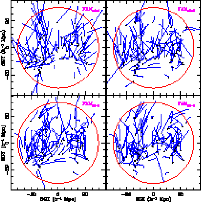
Figure 1:   2D projected reconstructed FAM orbits for different values of $N_{f}$. The black dots represent the final (present) positions for each object. The solid lines indicate the trajectories followed by the objects as a function of time. The top-left panel shows FAM reconstructed orbits with $N_{f}=1$ (Zel’dovich approximation). The top-right with $N_{f}=2$, the lower-left $N_{f}=3$ and the lower-right $N_{f}=6$.

In line with the above, the Zel’dovich approximation proved a highly versatile tool for the analysis of the cosmic matter flows. It was successfully applied to the nonlinear situation of mixed boundary conditions – tested and calibrated using $N$-body simulations – by Nusser et al. (1991) and Nusser & Dekel (1992). However, its validity remains restricted to the early stages of nonlinearity at which there is still a linear and direct relation between velocity and gravity field. Once matter inside the emerging structures starts to reach densities so high that local interactions become dominant, the Zel’dovich scheme quickly ceases to lose its applicability. Once matter elements start to cross each each others path the interaction between the nonlinear matter concentrations within the realm of the contracting structure will more and more deflect the orbits away from their initial linear trajectory. The linear kinematics of the Zel’dovich approximation will therefore no longer be able to follow the orbits of the matter elements. Higher order approximations based on perturbation theory have been advocated in order to follow such more advanced nonlinear circumstances. However, the improvement over simple first order Zel’dovich approximation turns out to be quite limited and not warranting the effort invested at each successive perturbation step. This is particularly so as with the onset of nonlinearity the rate at which successive perturbative orders terms become significant rapidly accelerates.

3.2 Least Action Principle in Cosmology

In more advanced nonlinear circumstances we encounter a more generic dynamical situation than a simple initial value problem. Typically, one seeks to compute the velocity field consistent with an observed density structure at the present epoch or, reversely, one deduces the density from the measured peculiar galaxy velocities. In the case of generic systems, the dynamical evolution represents a mixed boundary condition problem. This implies the system to be sufficiently constrained by complementing the incomplete dynamical information regarding the initial conditions with that pertaining to the dynamical state of the system at a different epoch. While $N$-body codes are particularly concerned with the ideal circumstances usually embodied in terms of initial value problems, a different kind of technique needs to be invoked to exploit the typical mixed boundary information yielded by observations.

A more profound and direct exploitation of the available information to follow the physics of such a cosmological nonlinear system was forwarded by Peebles (peebles89 (1989), peebles90 (1990)). He pointed out that finding the orbits that satisfy initial homogeneity – and by implication vanishing initial peculiar velocities – and match the (present-day) observed distribution of mass tracers constitutes a mixed-boundary value problem. Such problems lend themselves naturally to an application of Hamilton’s principle. This naturally leads to the formulation of the Least Action Principle (also known as “Numerical Action Method”), based on a variational analysis of the action $S$ of an isolated system of $M$ particles, which at a cosmic expansion factor $a(t)$ is given by

$$S\ =\ \int_{0}^{t_{0}}Ldt\ =\int_{0}^{t_{0}}dt\ \sum_{i}\ [{1\over 2}m_{i}a^{2}{\dot{\bf x}}_{i}^{2}-m_{i}\,\phi({\bf r}_{i})\ ]\ ,$$ (6)

in which $L$ is the Lagrangian for the orbits of particles with masses $m_{i}$ and comoving coordinates $x_{i}$ and corresponding peculiar gravitational potential $\phi({\bf x})$. For a system of particles interacting by gravity alone, embedded within a uniform cosmological background of density $\rho_{b}(t)$, this yields the following explicit expression for the action $S$,

$$S\ =\ \int_{0}^{t_{0}}dt \ \Bigl{[}\, \sum_{i}\,{m_{i}a^{2}\over 2}\left({d{\bf x}_{i}\over dt}\right)^{2}+\ {G\over a}\sum_{i\not=j}{m_{i}m_{j}\over|{\bf x}_{i}-{\bf x}_{j}|}+$$ (7)

$$\ +\ {2\over 3}\pi G\rho_{b}a^{2}\sum m_{i}{\bf x}_{i}^{2}\,\Bigr{]}$$

The exact equations of motion for the particles are then obtained from finding the stationary trajectories amongst the variations of the action $S$ subject to fixed boundary conditions at both the initial and final time.

Confining oneself to a feasible approximate evaluation in this Least Action Principle approach, one describes the orbits of particles, ${\bf x}_{i}(t)$, as a linear combination of suitably chosen universal functions of time with unknown coefficients specific to each particle presently located at a position ${\bf x}_{i,0}$. For instance, by using the linear growth mode $D(t)$ as time variable (Giavalisco et al. giav93 (1993), Nusser & Branchini nusbran (2000)), one can parametrize the orbit ${\bf x}_{i}(D)$ of a particle as

$${\bf x}_{i}(D)\ =\ {\bf x}_{i,0}\ +\ \sum_{n=1}^{N_{f}}\ q_{n}(D)\ {\bf C}_{i,n}\ ,$$ (8)

where the functions $q_{n}(D)$ form a set of $N_{f}$ time-dependent basis functions. The factors ${\bf C}_{i,n}$ are then a set of free parameters, whose value is determined from evaluating the stationary variations of the action.

The functions $q_{n}(D)$ satisfy both two orbital constraints, necessary and sufficient to define solutions in agreement with evolution in the context of the Gravitational Instability theory for the formation of structure in the Universe: $q_{n}(1)=0$ ensures that at the present time the galaxies are located at their observed positions ${\bf x}_{i}(1)={\bf x}_{i,0}$ and $\lim_{D\to 0}D^{3/2}q_{n}(D){\bf\theta}(D)=0$ guarantees vanishing peculiar velocities at early epochs which, in turns, ensures initial homogeneity.

3.3 Fast Action Minimization

The successful application of the Least Action Principle towards probing the kinematics and dynamics of an evolving cosmological system depends to a large extent on the specific implementation. This will be dictated by the characteristics of the physical system. In order to enable a meaningful LAP analysis of large samples of galaxies, like the Local Universe samples studied in this work, an optimized procedure is necessary for dealing with the large number of objects. Nusser & Branchini (nusbran (2000)) developed an optimized version of Peebles’ original LAP formalism, the Fast Action Minimization method. The various optimization aspects of the FAM implementation proved to be crucial for our purposes. The relevant optimization hinges on four major aspects of the FAM scheme.

The first FAM improvement involves the choice of time basis functions $q_{n}(D)$. Its convenient choice of time basis functions yields a simple expression for the action of the system and for its derivatives with respect to ${\bf C}_{i,n}$. Both quantities relate to the internal gravity term ${\bf g}_{int}$ of the system. Once the action and its derivatives are evaluated numerically, the minimum of the action is determined by means of the conjugate gradient method (Press et al. press (1992)). The orbits of the system are then fully specified through the set of parameters ${\bf C}_{i,n}$ found in correspondence to the minimum.

Closely related to the first aspect is that of tuning the choice of the time basis functions $q_{n}(D)$ such that only a limited number $N_{f}$ of basis functions is needed to successfully parameterize the orbits of the system. This is in particular beneficial to the the physical configuration we are studying here, involving Megaparsec scale dynamics characterized by quasi-linear or mildly nonlinear motions.

Note that using the growth factor $D$ as time variable makes the equations of motions almost independent of the value of $\Omega_{m}$ (Nusser and Colberg 1998). As a consequence FAM orbits and peculiar velocities in a generic $\Omega_{m}$ universe can be obtained by appropriate scaling those assuming a flat cosmology.

A final major aspect of the FAM implementation involves the efficient computation of the internal (self-consistent) gravity ${\bf g}_{int}$ from the particle distribution in the sample. To this end, the gravitational forces acting on the particles at the different epochs are computed by means of the TREECODE technique (Bouchet & Hernquist bouchet (1988)). By proceeding in this fashion, the FAM method is able to reconstruct the orbits of $\approx 10^{4}-10^{5}$ mass tracing objects back in time. This makes FAM numerically fast enough to perform a large number of orbit reconstructions, essential for performing the intended statistical analysis presented in the following sections.

In this work we use $N_{f}=6$ basis functions to parameterize the orbits, choosing a tolerance parameter $tol=10^{-4}$ to search for the minimum of the action $S$ and setting a softening parameter of $0.27h^{-1}{\rm Mpc}$ to smooth the gravitational force in the TREECODE. Orbit searching in dynamically relaxed systems is a difficult exercise since one has to choose among the many solutions found at the extrema of the action. However, since the purpose of FAM is to investigate large scale dynamics dominated by coherent flows rather than virial motions, our evaluations translates into an orbit search restricted to solutions which do not deviate too much from the Hubble flow i.e. to the simplest orbits that represents the minima of the action. Therefore, we set the initial guess for ${\bf C}_{i,n}$ according to linear theory prescription and search for the minimum of the action to avoid multiple solutions found a stationary points which typically describe passing orbits (Peebles peebles94 (1994)). We have checked that this choice of parameters is optimal in the sense that decreasing $tol$, increasing $N_{f}$ or changing the input set of ${\bf C}_{i,n}$ does not modify the final results appreciably.

Distortions in the resulting FAM-predicted peculiar velocities mainly arise from two systematic artifacts (Branchini, Eldar & Nusser branchini02 (2002)). One is the discrete sampling of the mass distribution within $V_{int}$. The second, and overriding one, is the failure of FAM in reproducing the virial motions within high-density regions that is a direct consequence of having considered solutions that represents perturbations to the Hubble flow. This deficiency of the FAM reconstructions is clearly illustrated by the residual velocity vector maps (see eq. 20) in Fig. 7 and Fig. 8 (bottom row). These show the velocity vector differences between the “real” measured, i.e. $N$-body, velocities and the corresponding FAM reconstructions (here based on either the galaxy distribution in a $30h^{-1}{\rm Mpc}$ central region or the extended $100h^{-1}{\rm Mpc}$ region). The maps show how the largest residuals are the ones found in the high density regions: although the FAM₃₀ and FAM₁₀₀ velocity fields do show pronounced velocities near these regions they are not the proper “real” virialized velocities they should have been. The residual fields thus underline the fact that FAM’s inaptitude to deal with regions characterized by large virial motions. Instead, in those situations it will lead to a false prediction of coherent inward streaming velocities, an effect pointed out by Nusser & Branchini (nusbran (2000)) and which can be also noted in our images when carefully studying them.

Finally, for practical reasons, since we are merely interested in measuring the effect of external gravity fields we make a further simplifying hypotheses. We ignore redshift distortion effects by working in real space In this respect, we should point out that extensions of the action principle method allowing a direct processing of redshift space information have been proposed and shown to work (Phelps phelps2000 (2000), Phelps phelps2002 (2002), also see Sharpe et al. sharpe (2001)).

3.4 The role of biasing

In this work we perform orbit reconstructions by assuming that all the mass of the systems is associated to point mass objects. More explicitly, we are making two different hypotheses. The first one is that we are able to identify a set of objects that trace the underlying mass density field in an unbiased way. The second one is that the internal structure of these objects is irrelevant for our reconstruction purposes.

The first assumption hardly applies to real galaxies that are most likely to be biased tracers of the mass distribution, as indicated by the relative bias between galaxies with different luminosities, colors and morphological type (Loveday et al. 1995). However, if galaxies and mass particles share the same velocity field so that the biasing relation remains constant along the streamlines, then the problem can be easily circumvented by specifying the biasing scheme at the present epoch (Nusser and Branchini 2000).

Within the standard lore of galaxies embedded in a virialized halo of dark matter that grow through hierarchical merging of smaller systems, neglecting the internal structure of objects is an assumption that is best justified a posteriori by showing how well Numerical Action methods can reproduce N-body velocities. Although the goodness of this assumption has been quantified by a number of numerical tests (e.g. Nusser and Branchini (2000) and Branchini Eldar & Nusser (2002)) little effort has been devoted to understand why numerical action methods can accurately reconstruct the velocity field of a large N-body simulation.

One of the reason for this success is that only $\sim 5\%$ of the points used in our reconstructions, that were randomly selected from the N-body simulation, belong to virialized regions where FAM reconstruction fails. Fortunately, the locality of this “virial effect” allows us to partially circumvent this problem by applying a modest spherical tophat smoothing of $2h^{-1}{\rm Mpc}$ to the FAM-predicted velocities. This tophat filter has been specifically important for the quantitative aspects of our study, where such systematic problems may sort distorting conclusions. This smoothing has been invoked in quantitative comparisons between FAM and $N$-body velocities presented in this work, in particular in the regression analyses.

Little is known about the ability of numerical action methods to reconstruct the orbits of virialized systems. Indeed, when applied to extended objects rather than point masses, numerical action methods follow a single center of mass point per virialized objects, completely neglecting its merging history. Some argument can be given to back our choice of neglecting the internal structure of virialized objects. First of all, after tracing back the merging history of virialized halos in N-body experiments a simple visual inspection reveals that particles ending up in the same halo at z=0 are contained within regions with simple boundaries at high redshifts. As a consequence, high order terms in the gravity potential about the halo center of mass are probably rather small. This probably minimize the role of major mergers whose rate for galaxy-size halos peaks in the redshift range 2-4 (Volonteri, Haardt and Madau 2003) while peculiar motions mostly develop at $z<2$ (Branchini and Carlberg 1994). These qualitative arguments clearly need to be confirmed by appropriate numerical analyses similar to that of Branchini and Carlberg (1994) but extending out to scales of cosmological interest.

3.5 Ordered reconstructions

To obtain an idea of the level of improvement obtained through the use of successively higher order FAM evaluations, Figure 1 depicts 2D projections of the corresponding FAM particle orbit reconstructions within a local spherical volume of $\approx 30h^{-1}{\rm Mpc}$. The black dots indicate the positions for each object in the sample, while the lines emanating from each dot represent the computed trajectories followed by these objects as they moved towards their present location. The illustrated configuration is taken from one of constructed mock catalogs, and resembles that of the Local Universe (see section 5.2.1). Each successive FAM reconstruction is based on the same (present-day) particle distribution. The four frames correspond to successively higher order FAM approximations, involving an increasing number $N_{f}$ of basis functions $q_{n}(D)$. The top-left panel shows FAM reconstructed orbits with $N_{f}=1$, which in fact corresponds to the conventional first order Zel’dovich approximation and thus represent the orbits that would have been obtained by the PIZA method (Croft & Gaztañaga croftgazt (1997)). These are followed by panels with $N_{f}=2$ (top right), $N_{f}=3$ (bottom left) and $N_{f}=6$ (bottom right). They show a clear and steady improvement towards the $N_{f}=6$ FAM evaluation. Testing proved that even higher order computations did not yield improvements significant enough to warrant the extra computational effort.

In summary, the galaxy orbits in our Local Universe environment are found at a minimum of the action which is not too far, yet different, from linear theory predictions. The FAM technique thus yields a significant modification of the recovered galaxy orbits and peculiar velocities for configurations that evolved well beyond the linear regime (see e.g. Figure 1). Potentially its ability to deal with nonlinear circumstances might even prove of benefit to recover sets of cosmological initial conditions satisfying nonlinear observational constraints at the present day, which indeed has been suggested by Goldberg & Spergel goldsperg (2000).

3.6 LAP and External forces

The original cosmological Least Action Principle formulation by Peebles ( peebles89 (1989)) considered a fully self-consistent, i.e. isolated, system of point masses. For practical reasons, the original implementation had to be restricted to systems of at most a few dozen objects. Almost exclusively, the Local Group of galaxies formed the focus of these LAP studies (Peebles peebles89 (1989), peebles90 (1990), peebles94 (1994), Dunn & Laflamme dunnlaf93 (1993)).

While these studies did indeed yield a substantial amount of new insight into the dynamical evolution of the Local Group, the issue of incorporating the dynamical influence exerted by external mass concentrations remained a major unsettled question. External forces do represent a significant component of the dynamics of the Local Group, as had been shown by Raychaudhury & Lynden-Bell ( raychlynd (1989)). They established beyond doubt that the Local Group cannot be considered a tidally isolated entity, and demonstrated that the Local Group is acted upon by an appreciable quadrupolar tidal force. The resulting tidal torque appears to be responsible for the large angular momentum of the Local Group as a whole, as Dunn & Laflamme (dunnlaf93 (1993)) showed in an elegant and pioneering analysis using orbits computed by the LAP variational method. They confirmed that the tidal influence of the external matter distribution is indeed essential to explain its present angular momentum.

In the course of time various strategies emerged to include external dynamical influences. The nature of these methods are mainly set by the character of the physical system under consideration, and to some extent was dependent on the available computational resources. Three strategies are outlined below.

3.6.1 Directly Including External Masses

To incorporate the external tidal influence within the LAP analysis the work by Peebles (peebles89 (1989), peebles90 (1990), peebles94 (1994)), Peebles et al. peebles2001 (2001) and Dunn & Laflamme (dunnlaf93 (1993)) attempted to identify a few principal external mass concentrations which would be responsible for the major share of the external gravitational influence. While in his first LAP study Peebles (peebles89 (1989)) considered the Local Group mainly as an isolated system, sequel studies (Peebles peebles90 (1990), Peebles et al. peebles2001 (2001)) attempted to assess the possible external influence by neighbouring matter concentrations. In Peebles peebles90 (1990) he attempted to condense the external tidal force into two nearby mass concentrations, the Sculptor and Maffei group, each modeled as a single mass. Both were incorporated as 2 extra particles, with properly scaled masses, within the action $S$ in order to take them along in a fully self-consistent variational evaluation. A similar approach was followed by Dunn & Laflamme (dunnlaf93 (1993)), be it that they included five galaxies/groups in the local cosmic neighbourhood which arguably contribute a significant torque on the Local Group. Also in a later application (Peebles et al. peebles2001 (2001)) this approach was followed, be it with an extensive outer region between $4h^{-1}_{75}$Mpc and $20h^{-1}_{75}$Mpc whose mass distribution was condensed into a coarse sample of some 14 major external objects.

This “self-consistent” strategy is feasible to pursue within the context of the original, computationally intensive, LAP implementation. This approach may therefore be followed in LG resembling situations in which a few objects suffice to represent the main aspects of a system’s dynamical evolution. On the other hand, cosmic systems of a considerably larger scale than the Local Group would in general be too demanding for. Supercluster sized regions, with scales of up to a few tens of Megaparsec, count many more individual objects than a galaxy group. These systems have also not yet reached a formation stage so advanced that they have already largely decoupled from the global Hubble expansion, so the resulting external gravitational influence is usually the shared responsibility of a large number of external matter concentrations. Accounting for the large-scale tidal field would quickly become prohibitively expensive in terms of the computational effort for conventional LAP analyses.

3.6.2 Inserting External Tidal Potential

An alternative strategy is to incorporate the external gravity in the LAP scheme via an approximate expression for the external contribution. This may be most directly achieved by inserting an extra external tidal potential term $\Phi_{tidal}(t)$ in the action $S$ (eqn. 6). As on sufficiently large, Megaparsec, scales we may expect this term to evolve according to linear gravitational instability perturbation growth,

$${\displaystyle\Phi_{tidal}(t)}\ =\ D_{\phi}(t)\ {\displaystyle\Phi_{tidal}(t_{0})}\ =\ {D(t)\over a(t)}\ {\displaystyle\Phi_{tidal}(t_{0})},$$ (9)

in which $\Phi_{tidal}(t_{0})$ is the tidal term at the present cosmic epoch and $D_{\phi}=(D/a)$ the linear growth term for the gravitational potential (the growth factor $D_{\phi}$ and cosmic expansion factor $a(t)$ are set to be equal to unity at the present epoch, $D(t_{0})=a(t_{0})=1.$). Thus, instead of evolving it self-consistently along with the considered system, the external field is determined at one epoch – usually the present one – and then incorporated as an extra linearly growing gravity field term $\Phi_{tidal}(t)$ in the action $S$:

$$S\ =\ \int_{0}^{t_{0}}dt \ \Bigl{[} \sum_{i}\,{\displaystyle m_{i}a^{2}\over\displaystyle 2}\left({\displaystyle d{\bf x}_{i}\over\displaystyle dt}\right)^{2}+\ {\displaystyle G\over\displaystyle a}\sum_{i\not=j}{\displaystyle m_{i}m_{j}\over\displaystyle|{\bf x}_{i}-{\bf x}_{j}|}+$$ (10)

$$\ +\ {\displaystyle 2\over\displaystyle 3}\pi G\rho_{b}a^{2}\sum m_{i}{\bf x}_{i}^{2}\ -\Phi_{tidal}(t)\,\Bigr{]}\,.$$

There are various possibilities to compute the tidal potential term $\Phi_{tidal}$, usually from the current mass distribution. One option is to compute it directly from a sample of $M_{ext}$ external objects which is deemed responsible and representative for the major share of the external tidal force field,

$$\Phi_{tidal}(t_{0})\ =\ \sum_{i}\ m_{i}\ \left\{{\displaystyle G\over\displaystyle a}\,\sum_{j=1}^{M_{ext}}{\displaystyle m_{j}\over\displaystyle|{\bf x}_{i}-{\bf y}_{j}|}\right\}\ .$$ (11)

Note that none of these external objects ($j=1,\cdots,M_{ext}$) is taken into account as far as the action of the system and the computation of their orbits is concerned, except for their “passive” role in determining $\Phi_{tidal}$. An alternative approach is to insert an approximate analytical expression for $\Phi_{tidal}$, in particular one including the dipolar and quadrupolar contributions, ${\bf d}$ and ${\bf T}$, to the tidal potential,

$$\Phi_{tidal}(t_{0})\ =\ \sum_{i}\ {\bf d}\cdot{\bf x}_{i}\ +\ {1\over 2}\,{\bf x}_{i}\cdot{\bf T}\cdot{\bf x}_{i}\ .$$ (12)

Equivalently, one may chose to insert the corresponding expressions directly into the expression for the derivative of the action with respect to an expansion coefficient, $\partial S/\partial C^{\alpha}_{i,n}=0$, evidently equal to zero within this variational approach.

The first, “direct”, procedure (eqn. 11) was followed by Shaya, Peebles & Tully (shaya (1995)), who for the purpose of studying the velocity field within the surrounding $30h^{-1}{\rm Mpc}$ modelled the relevant external mass distribution after the distribution of rich Abell clusters from Lauer & Postman (laupost (1994)). To some extent, Sharpe et al. (sharpe (2001)) operated along the same lines, be it that they added the resulting tidal term directly to the reconstructed velocities produced by the LAP procedure. However, while in principle exact, such a concentrated and static mass distribution may involve considerable uncertainties and can be highly sensitive to the uncertainties in the location of a few dominant point masses. As this spatial point distribution is supposed to form a suitable model for the underlying large scale matter distribution this may be even more worrisome.

Potentially more elegant may therefore be the modelling of a smooth tidal field along the line of the second procedure (eqn. 12), as suggested by Schmoldt & Saha (schmoldtsaha (1998)). The corresponding dipolar and quadrupolar term may then be based on the best available determinations of these parameters. On the other hand, when the LAP volume is comparatively large, the analytical approximation may represent an oversimplification of the force field, neglecting potentially important local variations within the external force field.

3.6.3 Selfconsistent and Direct FAM approach

The indirect “potential” approach which we described above (eqn. 11 or eqn. 12) may not properly account for the temporal evolution of the external field in the case of nonlinearly evolving systems. The formalism assumes a static, merely linearly evolving, gravitational potential. However, the matter concentrations which generate the external tidal forces will themselves get displaced as the cosmos evolves. These displacements may be relatively minor for distant masses, but for the more nearby entities this may be entirely different. A detailed treatment of the external mass distribution will be necessary when the influence of the nearby external objects on the evolution of small “interior” regions is comparable to or even dominant over the selfgravity of the region. It will be equally crucial to follow the detailed whereabouts of nearby matter concentrations in the case of a large “interior” region in which a marked contrast between the central regions and the outer realms may result in a significantly different dynamic evolution.

This prompted us to follow an alternative and direct approach, a fully self-consistent strategy in which also the external matter concentrations are accounted for in the computation of the system of evolving particle orbits. Alongside that in the “local” region for which we seek to reconstruct the velocity field, also the system of objects in the exterior regions ($30h^{-1}{\rm Mpc}<r<100h^{-1}{\rm Mpc}$) are considered. Non-uniform manifestations of the external influence can only be included by pursuing such a direct and systematic approach. It is only through the availability of the FAM technology that we were enabled to do so for a Megaparsec system consisting of a large number of objects.

Table 1: $N$-body simulation parameters. Column 1: cosmological model. Column 2: $\Omega_{0}$ mass density parameter. Column 3: $\Lambda$, cosmological constant parameter. Column 4: $\Gamma$, power spectrum shape parameter. Column 5: $\sigma_{8}$, density perturbation amplitude spectral normalization. Column 6: size of the computational box in $h^{-1}{\rm Mpc}$. Column 7: number of particles in the simulations.

Cosmology	$\Omega_{0}$	$\Lambda$	$\Gamma$	$\sigma_{8}$	boxlength	Nobj
$\Lambda$CDM	0.3	0.7	0.25	1.13	345.6	1923
$\tau$CDM	1.0	0.0	0.25	0.55	345.6	1923

4 Cosmological scenarios

The mock catalogs on which we apply our Fast Action Minimization analysis are extracted from $N$-body simulations in two different cosmological settings. Their characteristics, in terms of their relevant parameters, are listed in Table LABEL:table:parameters. The table also lists the simulation specifications. The first scenario is a flat $\Lambda$CDM model with a cosmological constant term $\Omega_{\Lambda,0}\leavevmode\nobreak\ =\leavevmode\nobreak\ 0.7$ ($\Omega_{0}=0.3,\,\Omega_{0}\leavevmode\nobreak\ +\leavevmode\nobreak\ \Omega_{\Lambda,0}=1.0,\,\Gamma=0.25,\,n=1$). The second model is a $\tau$CDM Einstein-de Sitter ($\Omega_{0}=1.0,\,\Omega_{\Lambda,0}=0,\Gamma=0.25,n=1$) model, motivated by the decaying particle model proposed by Bond & Efstathiou (bondef91 (1991)). Both scenarios were chosen to be viable with respect to the current observational constraints, implying similarities in many overall properties and appearances, yet with some significant differences with respect to their dynamical repercussions. This may provide indications on whether the galaxy motions in our local cosmic neigbourhood do contain information on the structure formation scenario.

In both cases the amplitude of density fluctuations is normalized on the basis of the observed abundance of rich galaxy clusters in the local universe. This abundance depends on the magnitude of the matter field fluctuations on the mass scale characteristic for galaxy clusters. This translates into a dependence on the amplitude of density fluctuations on cluster scales modulated by the mean global matter density. A variety of studies (e.g. White, Efstathiou & Frenk wef93 (1993), also see Eke, Cole & Frenk eke (1996)) found that in order to yield the present-day cluster abundance the amplitude of density fluctuations in spheres of radius $8h^{-1}{\rm Mpc}$, $\sigma_{8}$, and $\Omega_{0}$ are related by

$$\sigma_{8}=0.55\Omega_{0}^{-0.6}\,,$$ (13)

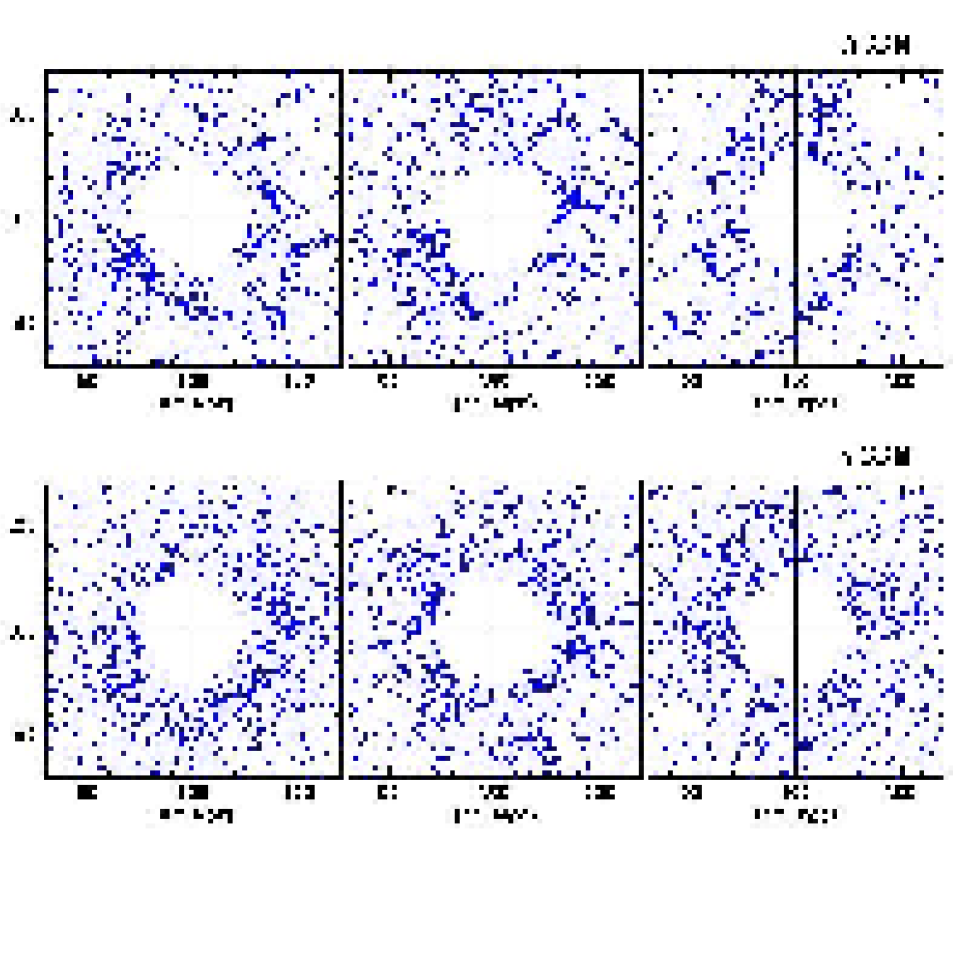
Figure 3: Central slices through a mock galaxy catalog realization. Depicted is the galaxy distribution in the external ($r>30\leavevmode\nobreak\ h^{-1}{\rm Mpc}$) volume. For each catalog, we show the $x-y$ (left), $x-z$ (centre) and $y-z$ (right) plane. Top row: $\Lambda$CDM mock catalog; Bottom row: $\tau$CDM catalog.

The resulting power spectra are depicted in Figure 2 (top left). On all scales, the density fluctuations in the $\tau$CDM scenario, represented by the dotted lines (for both $P(k)$ (green lines) and $k^{3}P(k)$ (blue lines)), are less pronounced than those of the $\Lambda$CDM scenario: the two power spectra have a similar shape and differ by a simple scaling factor over the entire wavelength range. Visually, this is immediately reflected in the stark differences between the spatial galaxy distribution in the resulting mock catalogs. Figure 3 provides such a visual comparison. It shows the “external” PSC$z$ catalog mimicking galaxy distribution in three mutually perpendicular central slices in the case of the $\Lambda$CDM scenario (top row), together with the same set of frames for a $\tau$CDM mock galaxy catalog (bottom row). On all scales, the $\tau$CDM galaxy distribution looks considerably more uniform than that in the $\Lambda$CDM Universe. Not only is the clustering of galaxies in the $\Lambda$CDM scenario more pronounced, it also delineates considerably larger structures, a manifestation of the power spectrum’s amplitude at the corresponding large wavelengths.

Because the higher average matter density in the $\Omega_{0}=1$ $\tau$CDM Universe does almost fully compensate for the lower amplitude of the density fluctuations the resulting gravity and velocity perturbation fields in the $\Lambda$CDM and $\tau$CDM scenarios are very similar. The velocity power spectra $k^{3}P_{v}(k)$ are shown in the bottom lefthand panel of Figure 2: their functional dependence is the same over the entire wavelength range. The larger mass corresponding to a given density excess in the $\tau$CDM Universe evidently effects a stronger gravitational force. The resulting large scale motions scale as $f(\Omega_{0})\propto\Omega_{0}^{0.6}$. This happens to be almost exactly the inverse of the average density perturbation amplitude scaling (eq. 13), which is proportional to $\Omega_{0}^{-0.6}$ (eqn. 13). While this is exactly the factor involved in the normalization of the power spectrum, in terms of $\sigma_{8}$, the lower level of density fluctuations gets precisely compensated by the higher amount of mass involved with them. This can be directly observed from the velocity power spectra $P_{v}(k)$ for the two scenarios (Fig. 2, lower lefthand frame). The velocity power spectra for both scenarios are exactly equal over the entire wavelength range, both in functional dependence as well as in amplitude. Note that also the gravity perturbations in the $\Lambda$CDM scenario are substantially stronger than those in the $\tau$CDM cosmology: because they scale with ${\scriptscriptstyle 3\over\scriptscriptstyle 2}\Omega H_{0}^{2}$ and the amplitude of the density perturbations, which according to eq. 13 is $\propto\Omega^{0.6}$, the average peculiar gravitational acceleration is proportional to $\Omega^{0.4}H_{0}^{2}$.

The comparison between $k^{3}P(k)$ (Fig. 2, top panel, blue lines) and $k^{3}P_{v}(k)$ (Fig. 2, bottom panel) in the same figure shows the shift of the velocity perturbations, with respect to the density perturbations, towards a more large-scale dominated behaviour. This follows directly from the continuity equation, connecting the velocity and density perturbations such that the velocity power spectrum relates to $P(k)$ through $P_{v}(k)\propto P(k)\,k^{-2}$.

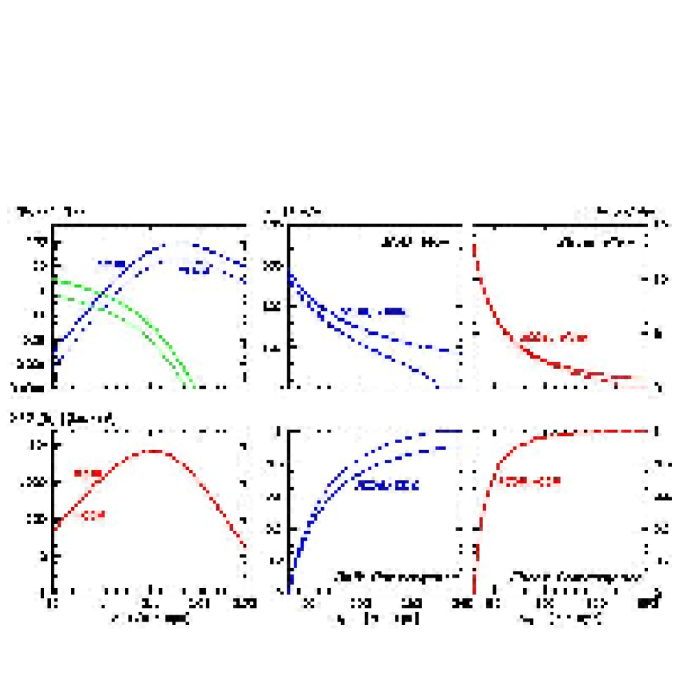
Figure 2: Spectral characteristics for the two studied cosmological scenarios. Upper left: Power spectrum $P(k)$ (green lines) and $k^{3}P(k)$ (blue lines), for the $\Lambda$CDM (continuous lines) and $\tau$CDM (dotted lines) cosmological scenarios used in this study. Lower left: velocity power $k^{3}P_{v}(k)$, the amount of velocity power per logarithmic waveband interval. Upper centre: expected bulk flow velocities ($\ {\rm km\leavevmode\nobreak\ s^{-1}}$) over a spherical (tophat) volume of radius $R_{TH}$. The solid line is the real theoretical prediction, the dashed one concerns the restricted power spectrum represented in the simulation box. Centre low: the convergence of the bulk flow, defined according to eqn. 16. Upper right: Expected shear flow $(\ {\rm km\leavevmode\nobreak\ s^{-1}Mpc^{-1}})$ over a spherical (tophat) volume of radius $R_{TH}$. Similar to bulk flow, the solid line concerns the full theoretical power spectrum while the dashed corresponds to the restricted power spectrum represented in the simulation box. Lower right: convergence of the shear flow, defined according to eqn. 16. Note that for the righthand frames the corresponding ordinate axis are the ones on the righthand side of the plotbox, while for the central frames it is the one on its lefthand side.

The large-scale behaviour of the (linear) velocity perturbation field immediately illuminates the difficulty in tracing the full array of matter inhomogeneities responsible for the cosmic motions within a specific cosmic region. To account for all noticeable contributions it is necessary to probe out to large depth. This is manifestly evident for the first order component in the externally induced flow, the “bulk flow” $v_{bulk}$. A measure for the expected bulk flow within a (tophat) spherical region of size $R_{TH}$,

$${\bf v}_{bulk}({\bf x})\,\equiv\,\int_{V}{\rm d}{\bf x}^{\prime}\,{\bf v}({\bf x}^{\prime})\,W_{TH}({\bf x}-{\bf x}^{\prime},R_{TH})\,,$$ (14)

is represented by the (root square) average value $\sigma_{v}$, whose value may be inferred from the Fourier integral

$$\sigma_{v}(R_{\rm TH}) \,=\, H_{0}f(\Omega_{0})\ \sigma_{-1}$$

$$\,\equiv\, H_{0}f(\Omega_{0})\ \sqrt{\int{\displaystyle{\rm d}{\bf k}\over\displaystyle(2\pi)^{3}}\,P({\bf k})\,{\hat{W}}_{TH}^{2}({\bf k})\,k^{-2}}\,.$$

In these relations, $W_{TH}({\bf x},R_{TH})$ and ${\hat{W}}_{TH}({\bf k})$ are the expressions for the tophat window filter, spatially and in Fourier space, and ${\bf\sigma_{-1}}$ is the spectral moment $\sigma_{j}$ for $j=-1$ (see Bardeen et al. bbks (1986), henceforth BBKS).

How substantial the large scale origin of the bulk flow is may be readily appreciated from figure 2 (top centre). Because the linear character of fluctuations on large scales, the spectral $\sigma_{v}$ (eq. 4) does provide a reasonable order-of-magnitude estimate of the magnitude of the large-scale bulk motions. The figure shows the estimated bulk flow amplitudes, $\approx\sigma_{v}$, as a function of the (tophat) window radius: the bulk flow is clearly a large scale phenomenon, converging only very slowly towards large spatial scales. In both the $\Lambda$CDM scenario and the $\tau$CDM scenario the externally induced bulk flow on a scale of $30h^{-1}{\rm Mpc}$ will be in the order of $200\ {\rm km\leavevmode\nobreak\ s^{-1}}$. Of this overall bulk flow, more than $100\ {\rm km\leavevmode\nobreak\ s^{-1}}$ has to be ascribed to inhomogeneities on scales exceeding $200h^{-1}{\rm Mpc}$ ! When assessing the motions in a local volume of $30h^{-1}{\rm Mpc}$ radius, in terms of relative external contributions, inhomogeneities on a scale larger than $100h^{-1}{\rm Mpc}$ still contribute more than $25\%$ of the total while the ones larger than $200h^{-1}{\rm Mpc}$ are still responsible for more than $10\%$ (see Fig. 2, centre bottom). We should therefore expect to find substantial external contributions in the $\Lambda$CDM and $\tau$CDM simulations. Note that this relative contribution to the bulk flow, the “bulk convergence”, is defined as the relative contribution by matter perturbations within a radius $R_{TH}$ to the externally induced bulk flow on a scale of $30h^{-1}{\rm Mpc}$ (the size of the NBG volume):

$${\cal F}_{\rm bulk}\,\equiv\,1\,-\,{\displaystyle\sigma_{v}(R_{TH})\over\displaystyle\sigma_{v}(30h^{-1}{\rm Mpc})}\,.$$ (16)

The second order aspect of the velocity field which we seek to study is the induced velocity shear $s_{ij}$,

$$s_{ij}\,\equiv\,{\displaystyle 1\over\displaystyle 2}\left\{{\partial v_{i}\over\partial x_{j}}+{\partial v_{j}\over\partial x_{i}}\right\}-{\displaystyle 1\over\displaystyle 3}(\nabla\cdot{\bf v})\,\delta_{ij}\,.$$ (17)

Also the velocity shear reveals interesting and distinguishing differences between the $\Lambda$CDM and the $\tau$CDM scenario. In the linear regime the expected magnitude of the shear tensor $s_{ij}$, on a tophat scale $R_{TH}$, may be evaluated through its direct proportionality to the tidal shear ${\cal T}_{ij}$. Quantifying $s_{ij}$ by means of its (root square ) average $\sigma_{s}$ (van de Weygaert & Bertschinger rienbert (1996)), we find

$$\sigma_{s}\,=\,H_{0}f(\Omega_{0})\,\sigma_{0}(R_{TH})\,\sqrt{\displaystyle 1-\gamma^{2}\over\displaystyle 15}\,$$ (18)

in which the (dimensionless) spectral parameter $\gamma\equiv\sigma_{1}^{2}/\sigma_{0}\,\sigma_{2}$ is defined through the $0^{th}$, $1^{st}$ and $2^{nd}$ spectral moments $\sigma_{j}$ (see BBKS bbks (1986)). The predictions for the two cosmological scenarios are shown in topright frame of Fig. 2. With respect to the bulk flow there is a marked difference in coherence scale: the major contributors to the tidal shear are located at considerably closer distances than the sources of the bulk flow (fig. 2, cf. lower right with lower centre). Most of the shear inducing matter inhomogeneities are found within a radius of $100h^{-1}{\rm Mpc}$, accounting for more than $95\%$ of its value (fig. 2, lower right). On a scale of $30h^{-1}{\rm Mpc}$ we expect an external tidal shear of $\approx 7\ {\rm km\leavevmode\nobreak\ s^{-1}Mpc^{-1}}$ for both the $\Lambda$CDM scenario and the $\tau$CDM model.

5 Mock catalog Construction and Analysis

5.1 $N$-body simulations

The two $N$-body simulations used in this work were carried out by Cole et al. (cole (1998)) within the context of an extensive study of PSCz catalogue resembling galaxy mock samples in a large variety of cosmological structure formation scenarios. They consist of $192^{3}$ particles in a computational box of $345.6\leavevmode\nobreak\ h^{-1}{\rm Mpc}$. They are dynamically evolved using an AP$3$M code in which the force is smoothed with a softening parameter of $0.27\leavevmode\nobreak\ h^{-1}{\rm Mpc}$.

The purpose of this study is a demanding task for truely representative $N$-body simulations. The $N$-body simulations should provide an optimal compromise between a high mass resolution on the small scale side and, on the large-scale side, a cosmic volume large enough to be dynamically representative. The large dynamic range requirement involves a mass resolution refined enough to resolve mass entities comparable to galaxies. This translates into an average inter-particle separation that needs to be smaller or comparable to that of galaxies in real observational catalogues. On the other hand, the simulations have to extend over a cosmic volume which is large enough to incorporate the major share of the gravitational influence exerted by the inhomogeneous cosmic matter distribution. Given the slow convergence of the bulk flow and its large coherence scale this is particularly challenging, and will be in the order of several hundreds of Megaparsec (see discussion in the previous section and fig. 2). Although hardly any current $N$-body simulations would fully fulfill the dynamic range requirements, the used $N$-body simulations do appear sufficiently adequate for a meaningful investigation of the relevant systematic trends and effects. This remains true in a qualitative sense, even though on the basis theoretical arguments (see e.g. Fig. 2) and observational indications (e.g. Hudson et al. hudsv (2004)) we know there may be substantial bulk flow contributions stemming from even larger spatial scales.

In this respect it is important to note is that the mock catalog realizations in this work are constrained by the finite size of the simulation box. The practical repercussions of being confined to a limited simulation volume may be inferred from the dashed curves in Fig. 2. They show the corrections to the expected bulk flow and velocity shear predictions (solid curves) when only the inhomogeneities in the restricted volume of the $345.6\leavevmode\nobreak\ h^{-1}{\rm Mpc}$ simulation box are incorporated. Because perturbations on scales exceeding the fundamental scale of the box are absent, the realized power spectrum has a rather sharp and artificial large-scale cutoff: the limited boxsize $L_{box}$ implies a cutoff in the power spectrum at low wavenumber $k_{box}=2\pi/L_{box}$. From Fig. 2 we can conclude that this correction is particularly apt for the bulk flow, predictions for the velocity shear seem hardly affected. As a consequence, on scales over $\approx 100\leavevmode\nobreak\ h^{-1}{\rm Mpc}$ the bulk flows in the realized $N$-body simulations will be severely repressed and far from representative. Although large-scale mode adding procedures have been proposed to partially remedy this situation (Tormen & Bertschinger torbert (1996) and Cole cole97 (1997)), our $\tau$CDM and $\Lambda$CDM simulations did not include such MAP (mode adding procedure) extensions. Conclusions with respect to the convergence of the FAM reconstructed velocity flows should therefore be referred to with respect to the suppressed velocity power spectrum indigenous to our $N$-body simulations (notice that this dynamic range issue is truely cumbersome to nearly any study attempting to assess velocity flows in computer simulations).

5.2 Mock Catalog Construction

From the full $N$-body simulations we extract mock catalogs made to resemble the local Universe. The $\Lambda$CDM and $\tau$CDM $N$-body simulations are processed through specified observational masks to imprint the required characteristics on the resulting mock catalogs. We distinguish two types of mock catalogs. From each $N$-body simulation we extract ten different “local” mock catalogs mimicking the NBG catalogue and, with these “local” samples representing their interior, ten different “extended” samples resembling the PSC$z$ catalogue.

The “local” class of mock samples is meant to sample the mass distribution within a $30\leavevmode\nobreak\ h^{-1}{\rm Mpc}$ region in and immediately around the Local Supercluster. These catalogs constitute volume-limited galaxy samples mimicking the Nearby Galaxy Catalog of Tully (tullycat (1988)). Mock catalogs of the second type are designed to account for the mass distribution out to distances of $100\leavevmode\nobreak\ h^{-1}{\rm Mpc}$. These “extended” samples represent flux-limited samples, for which we take the IRAS PSC$z$ galaxy catalog (Saunders et al. saunders (2000)) as template. The PSCz sample is not only ideal for our purposes in that it covers one of the largest volumes of the Universe amongst the available galaxy redshift surveys, but also in that it concerns a survey covering a large fraction of the sky and involves a well-defined uniformity of selection. Assuming that on large linear scales IRAS galaxies define an unbiased tracer of the underlying dark matter, Hamilton etal hamilton2000 (2000) found that its real-space power spectrum is consistent with that of a COBE-normalized, untilted, flat $\Lambda$CDM model with $\Omega_{m}=0.3$ and $\Omega_{\Lambda}=0.7$.

In both flux-limited and volume limited samples the mass of mock galaxies have been rescaled to the value of $\Omega_{m}=0$ of the parent N-body simulations, listed in Table LABEL:table:parameters.

In Table 2 we have listed the main characteristics of all mock catalogs used in this work. .

Table 2: Characteristics of the mock catalogs. Column 1: label of the catalog. Column 2: cosmological model. Column 3: for each mock catalog type: number of generated catalogs. Column 4: average number of particles $\langle N_{obj}\rangle$ in each catalog. Column 5: external radius of the catalog in units of $h^{-1}{\rm Mpc}$.

Cosmology	Set	Number of	$\langle N_{obj}\rangle$	Maximum
		catalogs		radius
$\Lambda$CDM	NBG	10	2740	30
	PSC$z$	10	10900	100
$\tau$CDM	NBG	10	2803	30
	PSC$z$	10	11207	100

In constructing the mock samples galaxies were identified with N-body particles selected randomly, exclusively according to the catalog selection criteria. Therefore, we did not attempt to include bias descriptions to model possibly relevant differences in the spatial distribution of dark matter and galaxies. This is different from the original use of the simulations (Cole et al. cole (1998)), in which various bias descriptions were invoked to construct artificial galaxy samples whose two-point correlation function and large-scale power spectrum largely matched that of the APM survey (Maddox et al. apmmaddox (1996)). The analysis of the small-scale nonlinear power spectrum of the PSCz by Hamilton & Tegmark ( hamilton2002 (2002)) even implies the bias on small scales to be very complex, involving a scale-dependent galaxy-to-mass bias. We, however, prefer not to include an extra level of modelling prescriptions. Our interest concerns the kinematics and dynamics of the matter distribution in the Local Universe, and the velocities of galaxies are thought to reflect these almost perfectly: they are mere probes moving along with the underlying dark matter flows, irrespective of their particular bias relation with respect to the dark matter distribution. The sole strict assumption is therefore that of having no velocity bias (Carlberg et al. carl90 (1990)), which on the large-scale Megaparsec scales at hand should be a more than reasonable approximation.

5.2.1 Mock NBG catalogs

The mock NBG catalogs are obtained by extracting spherical volumes of $30h^{-1}{\rm Mpc}$ from the $N$-body simulation particle distribution. The positions of the spheres in the parent simulations are not random but chosen to mimic as close as possible the characteristics of a Local Group look-alike region. Therefore, each mock catalog is centered on a particle moving at a speed of $625\pm 25$ km s^-1, residing in a region in which the shear within $5h^{-1}{\rm Mpc}$ is smaller than 200 km s^-1, where the fractional overdensity measured within the same region ranges between -0.2 and 1.0.

The velocity vector of the central particles defines a Galactic coordinate system and a Zone of Avoidance. Particles within the Zone of Avoidance are removed and substituted with a population of synthetic objects distributed using a random-cloning technique (Branchini et al. branchini99 (1999)). The Zone of Avoidance [ZA] in the mock samples is designed to mimic that of the PSC$z$ catalog (Saunders et al. saunders (2000)) and is smaller than the one of the real NBG catalog (Tully tullycat (1988)).

Each spherical region contains on average $2\times 10^{4}$ particles. This set of particles is randomly resampled in order to produce an unbiased catalog of around 2800 objects, a number that matches that of the galaxies in the real NBG catalog (Table 2). This procedure preserves, within shot noise errors, density fluctuations and thus does not alter the orbit reconstruction.

These NBG mimicking mock catalogs define volume-limited galaxy samples, so that the number of objects within a distance $x$ therefore increases as $x^{3}$. This is indeed what the resulting realizations yield, as may be discerned from the central part of the corresponding histogram in Figure 4 ($x\leq 30h^{-1}{\rm Mpc}$).

5.2.2 Mock PSC$z$ catalogs

The second set of mock catalogs was obtained by carving out spherical regions of radius $100h^{-1}{\rm Mpc}$ from the $N$-body simulations. Each of these new mock samples is centered on the same central position as that of corresponding NBG mock catalogs, with which they share the objects within the central $30h^{-1}{\rm Mpc}$.

While the central $30h^{-1}{\rm Mpc}$ region coincides with the NBG mock sample, the particle distribution in the external region ($30h^{-1}{\rm Mpc}<x<100h^{-1}{\rm Mpc}$) is supposed to mimic that of galaxies in the flux-limited IRAS PSC$z$ catalog. To achieve this the objects beyond $30h^{-1}{\rm Mpc}$ were selected from the $N$-body particle samples according to the PSC$z$ selection function used by Branchini et al. (branchini99 (1999)):

$$\psi(x)=Ax^{-2\alpha}\left(1+\frac{x^{2}}{x_{\ast}^{2}}\right)^{-\beta}\quad\textrm{if }x>x_{s}\ .$$ (19)

In this expression $x$ is the distance of the galaxy in $h^{-1}{\rm Mpc}$, while the parameters have the values $\alpha=0.53$, $\beta=1.8$, $x_{s}=10.9h^{-1}{\rm Mpc}$, and $x_{\ast}=84h^{-1}{\rm Mpc}$ (Branchini branchini99 (1999)). The selection function $\psi(x)$ defines the relative number density of the galaxy sample with respect to the number density of the $N$-body particle simulation. While the number density of PSC$z$ galaxies is equal to that of the particles in the simulation at $10.9h^{-1}{\rm Mpc}$, the amplitude $A$ of $\psi(x)$ is normalized such that $\psi(10.9)=1$.

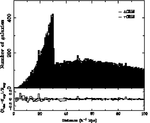
Figure 4: Object counts as a function of distance in the PSC$z$ mock catalogs. Upper panel: the two histograms show the average counts in the mock samples for the $\tau$CDM and $\Lambda$CDM cosmological models. The continuous line show the expected counts. Lower panel: the histograms show the fractional difference between the observed and expected counts averaged over all PSC$z$ mock samples in the two cosmological models explored.

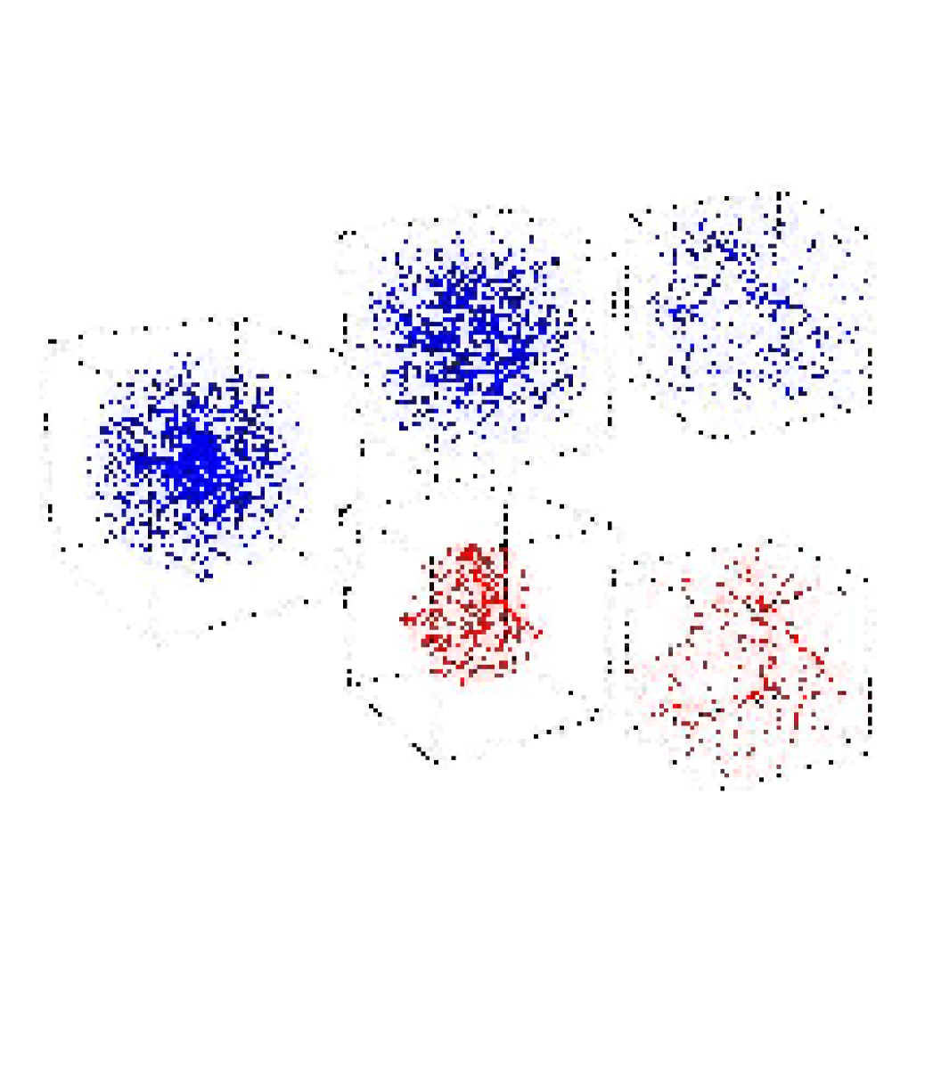
Figure 5: Compilation of cubic subregions and various mock subsamples of the object distribution in one of the $\Lambda$CDM PSC$z$ mock catalogs. The full mock catalog of objects, the PSCz look-alike volume and the NBG look-alike volume out to a radius of $100h^{-1}{\rm Mpc}$, is shown in the large lefthand cubic box (with size $200h^{-1}{\rm Mpc}$). The boxes along the top row and those along the bottom row represent mutually exclusive object samples. The lower ones represents the inner cosmic region ($x<30h^{-1}{\rm Mpc})$, the top row represent a corresponding part of the exterior PSCz region ($30h^{-1}{\rm Mpc}<x<100h^{-1}{\rm Mpc}$). Emanating from the complete cubic volume and running along the top row are two successive boxes which zoom in on the external PSCz mock catalog objects, with cubic sizes of $160h^{-1}{\rm Mpc}$ (middle right cube) and $80h^{-1}{\rm Mpc}$ (lower right cube) respectively. The lower row of two cubic volumes the central (inner) NBG mimicking object sample. The full inner sample, comprising a sphere of radius $30h^{-1}{\rm Mpc}$ is shown in the lower central cubic volume, whose size of $80h^{-1}{\rm Mpc}$ is equal to the central PSCz box, while the righthand cube focuses in on the $40h^{-1}{\rm Mpc}$ size central region.

Two additional steps concern the treatment of “Zone of Avoidance” objects and the evening of the matter density throughout the full external sample volume. A first step is the processing of sampled objects in the Zone of Avoidance such that the resulting sample conforms to a reality resembling situation. The ZA “removal$+$substitution” is implemented in the same way as in the case of the NBG mock catalog construction, with the replacement achieved with the same random-cloning technique. Finally, in order to guarantee a uniform average mass density throughout the volume, the mass of the objects in the flux-limited external object sample ($30h^{-1}{\rm Mpc}<x<100h^{-1}{\rm Mpc}$) has been scaled by the inverse of the selection function $\phi(x)$.

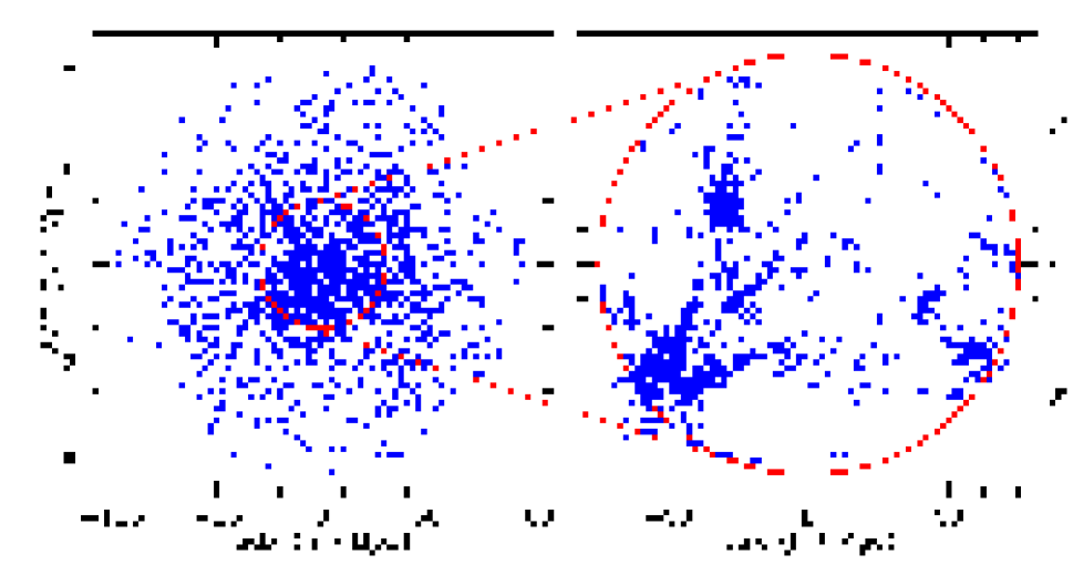
Figure 6: 2D projection of the particle distribution in one of the $\Lambda$CDM PSC$z$ mock catalogs (left panel). The inner circle divides the NBG look-alike volume limited region from the PSC$z$ flux limited one. The right panel show the 2D projected velocities in a slice of 10$h^{-1}{\rm Mpc}$ cut through the inner part of the catalog.

5.2.3 Mock catalog realizations

From both figure 5 and figure 6 one can obtain an impression of the spatial context of the local NBG mock sample within the wider environment of the surrounding $100h^{-1}{\rm Mpc}$ PSC$z$ sample. To visually appreciate the selection criteria of the catalogs, and their interrelationship, figure 5 shows a three-dimensional view of one set of the $\Lambda$CDM mock catalogs, extracted from the particle distribution in the $N$-body simulation of structure formation in a $\Lambda$CDM scenario. Emanating from the full PSC$z$ + NBG mimicking galaxy samples in the top righthand cube is a row of two cubes showing the content of the external PSC$z$ mock catalog (righthand) and the content of the central NBG mock catalog (lefthand). Figure 6 elaborates on this, and shows the projected particle distribution in the same PSC$z$ + NBG mock catalog (left panel) while focusing in on the central region (right panel). The circle (left panel) indicates the boundary of the volume-limited region comprised by the mock NBG galaxy sample, which in the right panel has been enlarged to show the corresponding velocity field within this NBG region. Velocities of objects within a 10$h^{-1}{\rm Mpc}$ thick slice are shown by means of arrows whose size is proportional to the amplitude of the galaxy velocity components within this slice.

As a matter of test, we checked the distance distribution of the resulting mock galaxy samples. The histograms of the resulting mock catalog distributions are shown in Figure 4. The upper part of Figure 4 shows the number of galaxies – averaged over all PSC$z$ mock catalogs for both two cosmological models – as a function of distance $x$ over the full range $x\leq 100h^{-1}{\rm Mpc}$. Clearly visible is the discontinuity at $30h^{-1}{\rm Mpc}$, marking the transition from volume-limited NBG-like region to the PSC$z$-like flux-limited outer region. For comparison, the solid line shows the theoretically expected counts (Eq. 19). The generated mock samples appear to match the expected distance distribution rather well. This is further underlined by the fractional difference between observed and expected counts, ${\rm N}_{\rm obs}/{\rm N}_{\rm exp}-1$, shown in the lower part of Figure 4. The fractional difference between mock samples displays a perfect featureless scatter pattern: Poisson noise free of systematic effects.

5.3 Mock Catalog Analysis

5.3.1 FAM velocity field reconstructions

On the basis of the FAM reconstructions of the galaxy velocities and the comparison with the true velocities – i.e. those in the original $N$-body simulation – we assess to what extent the matter distribution within the confines of each different mock galaxy sample does contribute to the total velocity of the galaxies. In these idealized circumstances of the $N$-body world the galaxy positions and velocities are known to perfect accuracy, thus circumventing the need to investigate the effects of measurement errors and deceptive systematic biases in the galaxy peculiar velocities. This should provide us with a better understanding of the nature and magnitude of genuine physical influences.

Three different velocities are accorded to each galaxy located within the “local” spherically shaped $30h^{-1}{\rm Mpc}$ NBG region. The first velocity is that of the “true”, $N$-body velocity. For each of the in total 20 NBG mimicking galaxy mock catalogs, the FAM reconstructions produce two additional velocity estimates. One FAM velocity results from the application of the FAM analysis to the restricted inner $30h^{-1}{\rm Mpc}$ NBG-like region itself. The second FAM based velocity is obtained on the basis of the FAM analysis on the extended, “full”, $100h^{-1}{\rm Mpc}$ PSC$z$ survey resembling sample (in which the “local” NBG sample occupies the interior central region). In the following, we will indicate these FAM velocities by the names of FAM₃₀ and FAM₁₀₀ velocities.

5.3.2 FAM₃₀ versus FAM₁₀₀ reconstructions

The mutual comparison between each of the three different galaxy velocities – the FAM₃₀, the FAM₁₀₀ and the full $N$-body velocities – is expected to yield abundant information on the dynamics and development of the structure in the interior $30h^{-1}{\rm Mpc}$ region:

The FAM₃₀ velocities are the galaxy velocities which would have been the product of the combined gravitational interaction of – solely – the matter concentrations within the central $30h^{-1}{\rm Mpc}$ volume. Any deficiency with respect to the “real” $N$-body velocity of each galaxy has to be ascribed to the gravitational impact of matter inhomogeneities outside the local NBG region.

By tracing the mass distribution further out to a distance of $100h^{-1}{\rm Mpc}$, invoking the matter distribution in the complete PSC$z$ mimicking mock samples, we will then evaluate the extent to which matter inhomogeneities within a 100$h^{-1}{\rm Mpc}$ scale are able to account for the motions within the local 30$h^{-1}{\rm Mpc}$ region. From this we can infer in how far the external influence over the local region can be ascribed to matter fluctuations situated between a radius of 30$h^{-1}{\rm Mpc}$ and 100$h^{-1}{\rm Mpc}$.

In this study we also have to take into account the fact that a single 30$h^{-1}{\rm Mpc}$ region cannot be considered representative for the whole Universe, and generic conclusions on the basis of the kinematics within a single 30$h^{-1}{\rm Mpc}$ volume cannot be drawn. This is also true for the the NBG mock samples in this work, even though they were selected according to some strict criteria (see section 5.2). Analysis and conclusions will therefore be based on a straightforward average over the 10 different $30h^{-1}{\rm Mpc}$ mock samples which were constructed for each cosmological scenario. The dispersion in the extracted parameter values will provide a reasonable estimate for their significance.

5.3.3 Analysis of Reconstructions

The basic product of the FAM reconstructions are velocity maps, in essence a velocity vector at the location of each galaxy in the sample. Our analysis consists of three different but complementary tracks. The first and most straightforward one is the visual inspection of the resulting velocity vector maps. It provides a direct impression of the extent to which a FAM reconstructed field reproduces the true velocities. Also, it will provide a direct impression of a spatial coherence in the differences between true and reconstructed field, which is an incisive way to uncover systematic contributions like e.g. a bulk flow component.

The second examination is a strictly local analysis, a pure point-to-point comparison between the velocities predicted by the FAM reconstructions on the one hand and the “true” $N$-body velocity of the same object on the other hand. To some extent, the analysis by means of scatter plots is the most direct and objective quantitative comparison between two fields. Various velocity related quantities will be assessed in this fashion. Note that these localized comparisons cannot address the presence of spatial coherence in the cosmic flows (even though they may uncover systematic effects caused by external influences).

Finally, the third track is targeted towards a factual description of the spatial coherence within the velocity fields or, rather, in the residual fields between the “true” velocities and the reconstructed velocities. Systematic trends in these residual fields are interpreted as manifestations of external forces. Of these we shall determine the first-order – bulk flow – and second order – velocity shear – components.

6 FAM velocity vector maps

For reasons of consistency and to achieve optimal transparency the illustrated velocity vector maps in the following discussion all concern the same mock sample of NBG calculations. For the illustration of the FAM₃₀ (Fig. 7) and the FAM₁₀₀ (Fig. 8) reconstructions we use one of the $\Lambda$CDM $30h^{-1}{\rm Mpc}$ NBG mock catalogs. It is the same galaxy sample that was shown in 3-D in Fig. 5 and in projection along the “x-y” plane in Fig. 6.

The vector maps in Figure 7 and Fig. 8 depict the projections of the raw unsmoothed galaxy velocities, for galaxies within a central slice of $10h^{-1}{\rm Mpc}$. The size of the arrows is proportional to the amplitude of the peculiar velocity component within this slice, each arrow starting at the location of the galaxy. Both figures consist of three successive rows. The velocity maps in the first row correspond to the “real” world of the $N$-body simulation. The second row depicts the velocity maps for the FAM reconstructions, the FAM₃₀ reconstruction in Fig. 7 and the FAM₁₀₀ reconstruction in Fig. 8. The last row shows the resulting residual velocity vector fields,

$${\bf v}_{\scriptstyle{\rm res}}\equiv{\bf v}_{\scriptstyle{\rm FAM}}-{\bf v}_{\scriptstyle{\rm Nbody}}\,,$$ (20)

the vector difference between the $N$-body velocities and the corresponding FAM velocity reconstructions, [$N$-body - FAM₃₀] and [$N$-body - FAM₁₀₀].

Each row has three panels, containing the vector maps in the three mutually perpendicular “central” slices. Each plane is identified by means of the index combination “x-y”, “x-z” or “y-z” (top figure), the index pair identifying the horizontal and vertical axis along which the panel is seen. Imagining these three planes passing through the centre of the $30h^{-1}{\rm Mpc}$ NBG volume provides a spatial impression of the full 3-D velocity field. Note that here the choice of Cartesian coordinate system does not have any special significance, arbitrarily set by the axes of the total $345.6h^{-1}{\rm Mpc}$ simulation box (the “fundamental” box) from which the mock catalogs were distilled. This is unlike vector maps (e.g. Fig. 13) in some later sections.

6.1 $N$-body sample: the “observed” velocities

The velocity vectors in the top row vector maps depict the “real” $N$-body velocities of the “galaxies” located within the three “central” slices (the same for Fig. 7 and Fig. 8). The galaxy distribution is characterized by a few dense, massive and virialized clumps, visible as high concentrations of large and randomly directed velocity vectors. The truely massive concentration visible in the lower left of the $x-y$ panel is part of a superstructure extending beyond the boundaries of the NBG region. It represents a major and dominant source for the motions in this area. This may be appreciated from the observed velocity flow towards this clump and the overall distortion of the flow in its vicinity. The large configuration visible in the “y-z” slice contains several dense compact regions embedded in a ridge-like structure running curvedly from the lower righthand corner to a location slightly left from the centre. At least partially related to this mass concentration in and around the ridge is the bulk flow along the right-to-left direction.

Overall, the “x-y” and “y-z” vector maps indicate the presence of a dominant coherent “bulk flow” pattern which can be traced throughout the whole NBG volume. By coincidence, the orientation of the coordinate axes is such that the direction of the bulk flow is almost perfectly aligned along the “y”-axis: for this particular mock sample the “y”-axis does represent a physically significant direction defined by the streaming pattern itself. The bulk flow seems to be directed towards some (fictitious) point outside the local $30h^{-1}{\rm Mpc}$ region.

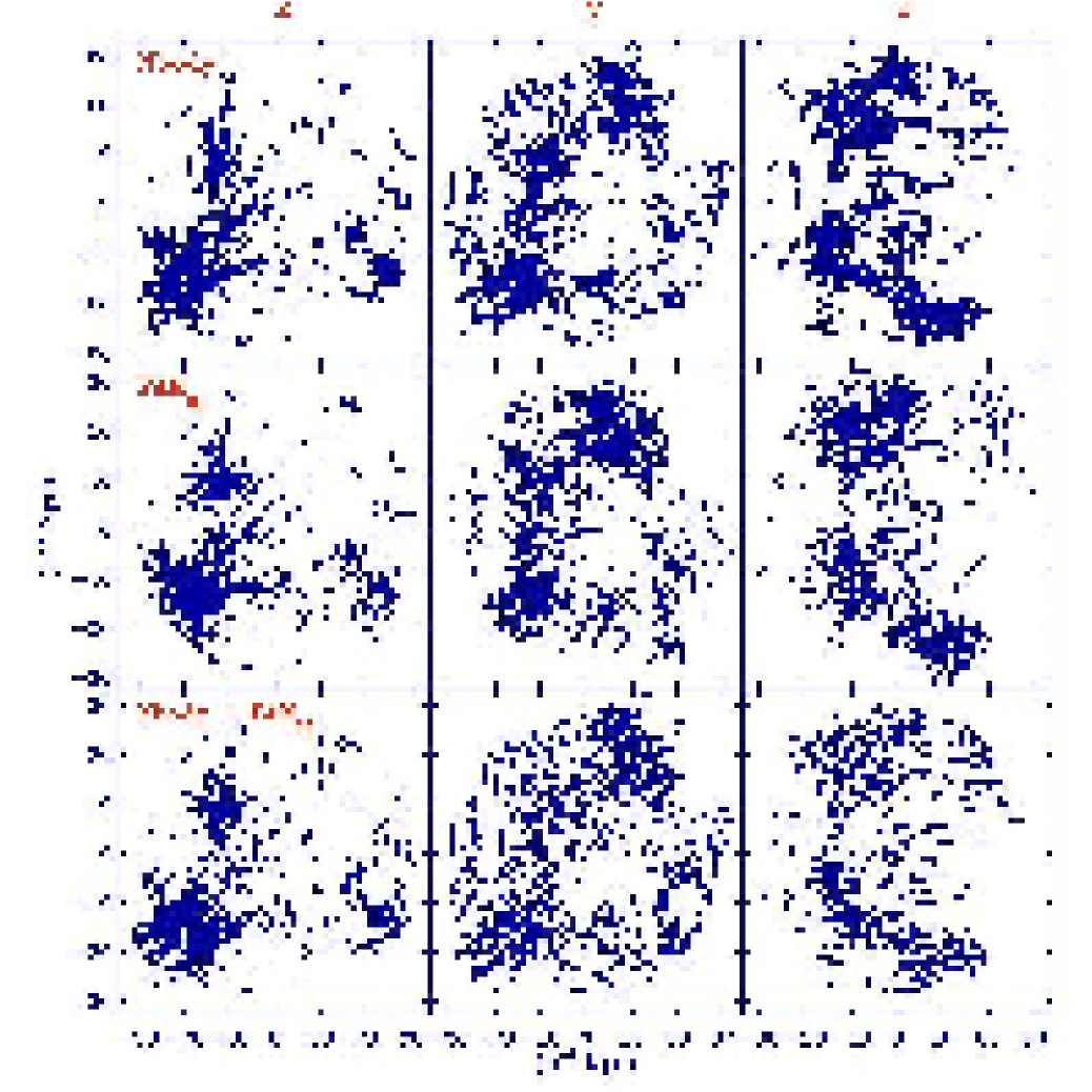
Figure 7: 2D projected, unsmoothed velocities at each particles position in one of the NBG-$\Lambda$CDM mock catalogs. Each row contains three frames, corresponding to the central $y-z$, $x-z$ and $x-y$ plane through the point sample. Bottom row: projected $N$-body velocities. Central row: projected FAM₃₀ velocities. Bottom row: residual $N$-body-FAM₃₀ velocities.

A dominant and conspicuous coherent flow pattern also characterizes the $x-z$ velocity vector map. While the flow in the two other planes seems to be almost exclusively dominated by a bulk flow, here the pattern has a more complex geometry, readily recognizable as a typical “velocity shear” pattern. The specific shearing motion in this plane consists of a compressional component along the top lefthand to lower righthand direction, in combination with a dilational stretch along the perpendicular direction from the lower lefthand towards upper righthand corner.

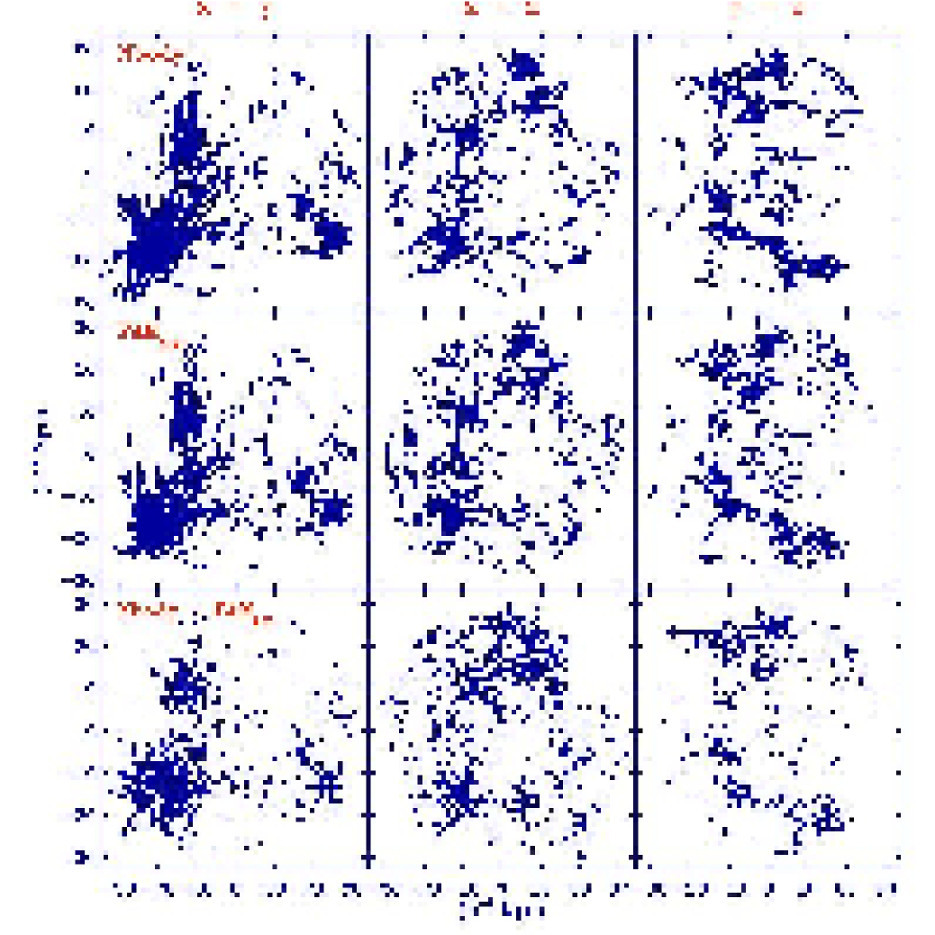
Figure 8: Same as Fig. 7, for the PSCz based FAM₁₀₀ reconstructions. Shown are the 2D projected, unsmoothed velocities at each particles position in the central NBG mimicking volume of the full PSCz-$\Lambda$CDM mock catalogs, the same region as depicted in Fig. 7. Each row contains three frames, corresponding to the central $y-z$, $x-z$ and $x-y$ plane through the point sample. Bottom row: projected $N$-body velocities. Central row: projected FAM₁₀₀ velocities. Bottom row: residual $N$-body-FAM₁₀₀ velocities.

6.2 NBG samples: FAM₃₀ velocity vector maps

The role of the local cosmic matter distribution on the motions in the local Universe is assessed on the based of the “FAM₃₀ velocities”. They are the peculiar velocities computed by FAM on the basis of the local matter distribution, supposedly reflected by the galaxies within the NBG catalogs. The corresponding reconstructed velocities are shown in the second panel row of Figure 7. With their final position as boundary condition, each velocity vector is located at the same galaxy position as in the $N$-body maps (top row). Note that the vector maps in Figure 7 and Figure 8, and also the later ones in Fig 12, Fig 13 and Fig 14, show the pure unsmoothed velocity vectors (and do not “correct” for the virialized regions).

The FAM₃₀ velocity maps are distinctly different from the corresponding $N$-body velocity maps (top row): a coherent flow pattern is almost entirely absent. The FAM₃₀ reconstructions obviously did not recover the strong bulk flow observed in the $N$-body velocity maps, nor the striking shear pattern in the $x-z$ plane. Because the FAM₃₀ velocity field reconstructions solely relate to the matter distribution within the inner 30$h^{-1}{\rm Mpc}$ NBG region, this indicates that the major share of coherent bulk flow and the velocity shear are due to the matter distribution outside the central 30$h^{-1}{\rm Mpc}$. This is most readily apparent in the velocity residual maps [$N$-body - FAM₃₀], the difference between the $N$-body and the FAM₃₀ velocity vector fields (bottom row of Fig. 7). In the residual field [$N$-body - FAM₃₀] we recognize the same characteristic flow patterns, strong spatial correlation, long-range coherence and overall morphology as in the full $N$-body velocity field. This represents convincing evidence for the external origin of the large-scale “bulk” and “shear” component in the local velocity flow.

Prominently visible in the residual velocity field is the strong bulk flow along the “y”-axis. Overall, the spatial pattern of the residual bulk flow appears to reproduce that of the $N$-body flow field. However, some minor yet significant differences between the residual and the full $N$-body bulk flow can be discerned. The amplitude of the corresponding velocities in the residual map is somewhat smaller than the equivalent $N$-body velocities: apparently part of the bulk flow is induced by the local NBG matter distribution. This does not seem to be true for the velocity shear: the shear patterns in the “x-z” plane of the residual and $N$-body velocity fields are almost identical (except for the virialized motions in high-density clumps). Apparently, the velocity shear component is almost exclusively due to external matter distribution. As a locally flattened matter configuration would induce an internal shear flow, this appears to imply a local matter distribution whose geometry is hardly flattened or elongated.

Closer inspection of the FAM₃₀ velocity field provides a more detailed view of the small-scale flow pattern mentioned above. In the “x-y” plane the large-scale ($N$-body) bulk flow has virtually completely disappeared. Instead, the dominant motion in the “x-y” plane is a streaming flow towards a prominent matter concentration within this region (lower left). On the other hand, in the “y-z” slice a trace of the $N$-body bulk flow along the “y” axis remains, be it that the corresponding velocities have considerably smaller amplitudes than their $N$-body counterparts. These local motions appear to be effected by the matter located along the lower ridge, supporting the impression that this feature is a local extension or outlier of the large-scale matter configurations responsible for the full bulk flow. Examination of the panels in Fig. 5 and Fig 6 indeed seems to suggest that the density ridge in the lower half of the “y-z” plane is indeed connected to structures just outside the NBG volume, while this perhaps may be true for the massive matter clump in the “x-y” plane too. This may not come as a surprise: the local matter distribution will to some extent be correlated with the external matter configuration so that the locally induced bulk flow is expected to reflect at least partially the full $N$-body bulk flow.

In summary, the inability of the FAM₃₀ reconstruction to recover the large-scale bulk flow and velocity shear is a consequence of the fact that they are a result of the action of the mass distribution on scales larger than the internal $30h^{-1}{\rm Mpc}$ size region while the FAM₃₀ velocities are entirely and self-consistently determined by the mass distribution within this interior region. The residual [$N$-body - FAM₃₀] maps, which are a model for the possible findings of a real-world observational campaign, provide the most elucidating illustration of their “external” origin. Even though they do provide convincing evidence for their external nature, they do not provide sufficient information to infer the identity and nature of the main source of the flow patterns. In principle, however, we may deduce a substantial amount of information on the basis of a careful quantitative analysis: the work by Lilje, Yahil & Jones (lilje (1986)) still sets a prime example. To this end, we will investigate the external matter distribution in the PSC$z$ $100h^{-1}{\rm Mpc}$ sized regions.

As a final note, we point to the rather artificial nature of velocity vectors in the vicinity of the massive clump in the “x-y” slice as indicative for the self-consistent nature of the FAM reconstructions. Its location near the edge of the NBG volume even appears to have generated the rather contrived infall motions along the rim of the NBG sphere.

6.3 PSC$z$ samples: FAM₁₀₀ velocity vector maps

The contribution by the relatively nearby external matter agglomerations, within a distance of $100h^{-1}{\rm Mpc}$, to the motions in the local Universe is investigated on the basis of the “FAM₁₀₀ velocities”. FAM produces these peculiar galaxy velocities on the basis of the galaxy sample in the full mock PSC$z$ galaxy sample, extending out to $100h^{-1}{\rm Mpc}$ around the center of our local region. The corresponding reconstructed velocities are shown in the second panel row of Figure 8. It is the analogy for the “FAM₁₀₀ velocities” of Figure 7, and concerns the same $30h^{-1}{\rm Mpc}$ central region (the NBG region is the central subregion of the PSC$z$ mimicking catalog). The FAM₃₀ maps showed the dominant influence of externally induced forces on the motions in the local 30$h^{-1}{\rm Mpc}$ NBG region: on the basis of the FAM₁₀₀ maps we seek to assess whether the major share of the responsible external matter agglomerations may be identified within the realm of a PSC$z$ like volume.

Comparison of the first and the second row of panels in Fig. 8 shows the large degree of similarity between the FAM₁₀₀ velocities (panels 2^nd row) and the $N$-body velocities (panels top row). Unlike the FAM₃₀ maps in Fig. 7 we find that the FAM₁₀₀ maps successfully reproduce most of the large-scale behaviour and most of the finer details of the $N$-body velocity field. The degree of similarity is particularly evident in the corresponding residual velocity field [$N$-body - FAM₃₀] (bottom row panels). With the exception of the high-density virialized regions the residual velocities are very small and mostly randomly oriented: no significant spatial correlations and spatial coherence can be detected.

The detailed similarity between the $N$-body and the FAM₁₀₀ maps shows that it is sufficient to take account of the mass distribution out to $100h^{-1}{\rm Mpc}$ for explaining, in considerable detail, the velocity flows in the local NBG volume. Moreover, the detailed rendering of the velocity field by FAM is a convincing demonstration of the capacity of the FAM technique to accurately describe the dynamics implied by the observed local galaxy distribution. The quantitative comparisons in the following sections will provide ample support to this claim.

Of course, the above conclusion is partially related to the realizations of the cosmological scenarios we have studied. The behaviour of the power spectrum $P(k)$ on large scales will considerably influence the generality of our findings. A power spectrum with more power on large scales would modify our findings: potentially it may be so that we need a representation of the matter distribution out to larger radii than $100h^{-1}{\rm Mpc}$. In this respect it is important to note that the used $N$-body velocity fields do not have any contributions from wavelengths larger than $\approx 175h^{-1}{\rm Mpc}$ (both for $\tau$CDM as well as $\Lambda$CDM simulations, see Fig. 2). This merely for the technical reason of the simulation box imposing an upper limit to the scale on which we can represent $P(k)$. The extent to which this may influence our conclusions may be readily appreciated from Figure 2 (right column, top and bottom panel: compare solid lines with dashed ones). The velocity field perturbations of $\tau$CDM and $\Lambda$CDM carry out considerably further than the fundamental scale of the simulation box, in particularly affecting the resulting bulk flows.

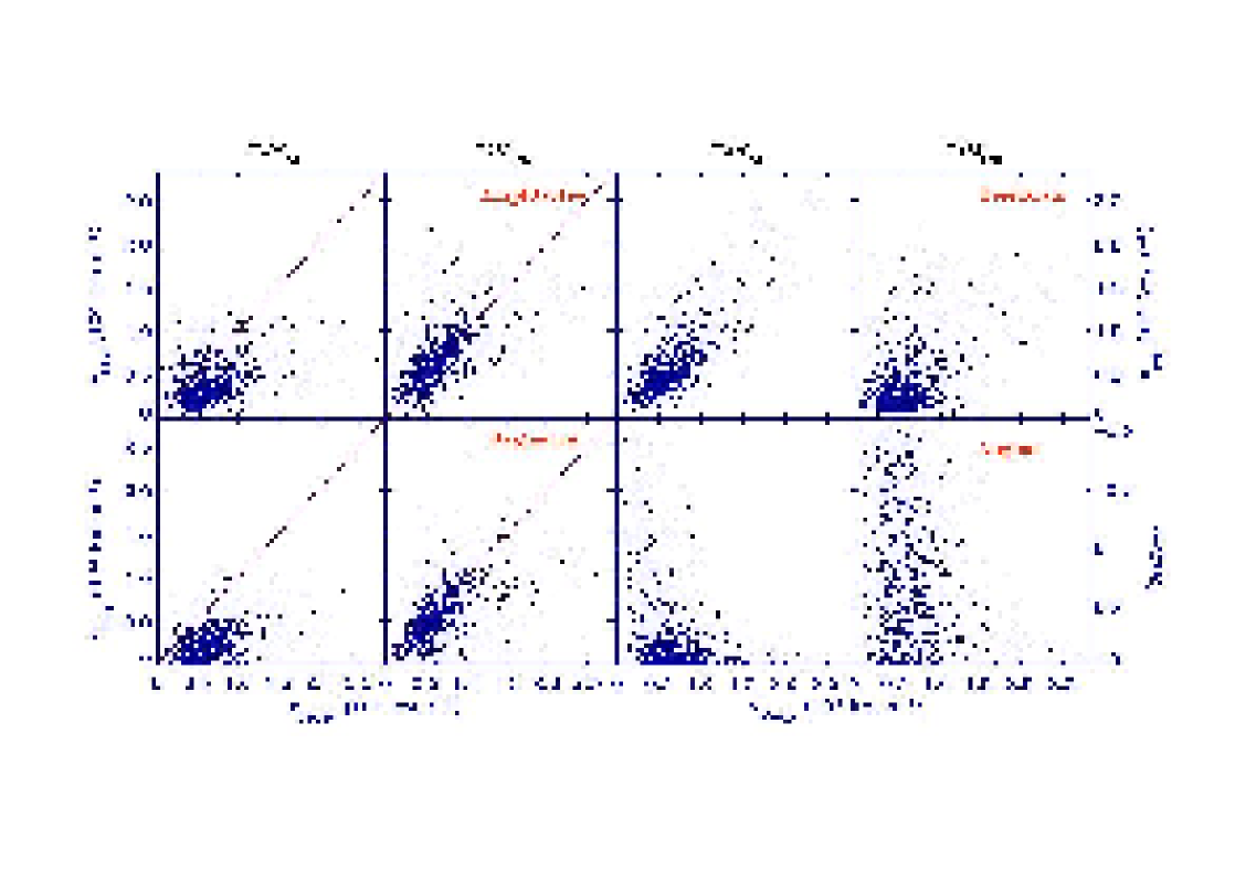
Figure 9: Point-to-point comparison (scatter plot) of four quantities related to FAM reconstructed velocities and the corresponding “real” object velocity in the underlying $N$-body samples. The $N$-body realization, and the mock sample, concern the $\Lambda$CDM scenario. For each quantity two panels are shown: the lefthand one is the one for FAM₃₀ reconstruction, the righthand one for the FAM₁₀₀ reconstruction. Top lefthand: the amplitude of the velocities. Top righthand: residual velocity amplitudes FAM-$N$-body. Bottom lefthand: FAM velocity component projected along the $N$-body velocity. Bottom righthand: angle $\theta$ between FAM velocity and $N$-body velocity, in terms of $\mu=\cos(\theta)$.

7 Point-to-point comparison

Scatter diagrams are used to assess the point-to-point comparisons between quantitative aspects of the “real” galaxy velocities in the original $N$-body samples and the computed velocities in the FAM₃₀ and FAM₁₀₀ reconstructions. This analysis is meant to be a direct, in principal local, assessment of systematic trends in the velocity flows in volume of the NBG sample. The comparisons involve a component of the “true” $N$-body velocity (abscissa) versus the equivalent quantity for either the FAM₃₀ or FAM₁₀₀ velocities, or of the corresponding residuals (ordinate). Since the objects had been artificially added to the Zone of Avoidance, any particles inside this region (see sec. 5.2.2) are excluded from these diagrams.

7.1 Systematics

If we neglect the small-scale sources in the deficiencies of FAM reconstructions, the differences between FAM₃₀ and FAM₁₀₀ scatter plots are mainly to be ascribed to the corresponding differences in the external gravitational influence acting over the two corresponding sample volumes. In the external gravitational influence the the corresponding leading velocity terms are the bulk flow ${\rm v}_{\scriptstyle{\rm bulk}}$ and the velocity shear $s_{ij}$,

$$v_{\scriptstyle{\rm Nbody},i}\,\approx\,v_{\scriptstyle{\rm FAM},i}\,+\,v_{\scriptstyle{\rm bulk},i}\,+\,\sum_{j=1}^{3}\,{s}_{ij}\,x\hat{x}_{j}\,+\,\ldots$$ (21)

In the above $i,j$ denotes the Cartesian component indices. The vectors $\hat{x}_{j}$ represent the vector components along the Cartesian $j$ direction of the spatial unity vector oriented along the object position vector ${\bf x}$. Following this definition, $x\hat{x}_{j}$ is the $j$-component of the position vector ${\bf x}$, with $x$ the distance of the object.

Systematic differences in FAM velocity-$N$-body velocity scatter diagrams are therefore to be attributed to differences in bulk flow, shear and possibly higher order contributions. Because each of these large-scale phenomena will manifest themselves in distinctly different ways, we seek to identify them from the scatter diagrams. An horizontal offset in the scatter diagram would be the trademark for a bulk flow component. Velocity shear would manifest itself as a distinctly characteristic correlation between residuals and velocities, although the prominence of this signal will be dictated by shear magnitude, configuration, and orientation with respect to the reference system (as is true for the bulk flow). In reality, the situation will be more intricate. Subtle correlations between small-scale and large-scale contributions will bring about a change in the slope of the scatter diagram of FAM reconstructed velocity components against their full $N$-body values (see 7.3.2).

7.2 Velocity Scatter Diagrams Analysis

Scatter diagrams are presented in three successive figures. The depicted scatter diagrams all relate to a $\Lambda$CDM mock catalogue, and each of these point-to-point analyses relates to a different aspect of the velocity field reconstructions. Figure 9 contains four different panels, of which each contains two scatter diagrams: FAM₃₀ versus $N$-body quantity (left) and the equivalent FAM₁₀₀ versus $N$-body quantity (right). The diagrams in Fig. 10 focus on the correlations between these quantities and the scatter around regression relations. The figure addresses three velocity-related quantities, each taking one column of each 2 panels: the top one for the comparison of the FAM₃₀ components with their $N$-body counterparts, and the same for the FAM₁₀₀ components in the bottom frame.

Table 3: Results of the linear regressions in the tests with the mock catalogs. Col. 1: Cosmological model. Col. 2: Component Col. 3: label of the set. Col. 4: the average Spearman (non-parametric) correlation coefficient Col. 5: average linear correlation index of the best fitting line and its $1\sigma$ scatter. Col. 6: average zero point of the best fitting line and its $1\sigma$ scatter. Col. 7: average slope of the best fitting line and its $1\sigma$ scatter. Col. 8: average dispersion around the fit and its $1\sigma$ scatter

Cosmology	Component	Set	$R_{Spear}$	$R_{lin}$	$a_{0}$	$a_{lrg}$	$\sigma_{lrg}$
					(km s-1)		(km s-1)
	$\mid v\mid$	FAM30	0.54 $\pm$ 0.11	0.56  $\pm$ 0.11	-29.43  $\pm$  84.28	0.66  $\pm$ 0.21	198  $\pm$  73
		FAM100	0.68 $\pm$ 0.12	0.62  $\pm$ 0.16	83.38  $\pm$ 156.39	0.85  $\pm$ 0.26	212  $\pm$  89
$\Lambda$CDM	$v_{\parallel}$	FAM30	0.43 $\pm$ 0.14	0.37  $\pm$ 0.20	-198.21  $\pm$ 173.86	0.65  $\pm$ 0.30	251  $\pm$ 114
		FAM100	0.59 $\pm$ 0.23	0.52  $\pm$ 0.29	-135.98  $\pm$ 242.78	0.99  $\pm$ 0.40	281  $\pm$ 158
	$v_{i}$	FAM30	0.54 $\pm$ 0.20	0.48  $\pm$ 0.29	19.35  $\pm$ 140.90	0.66  $\pm$ 0.25	240  $\pm$ 130
		FAM100	0.71 $\pm$ 0.27	0.61  $\pm$ 0.31	5.96  $\pm$   78.94	0.86  $\pm$ 0.23	233  $\pm$ 107
	$v_{res,i}$	FAM30	0.65 $\pm$ 0.11	0.66  $\pm$ 0.11
		FAM100	0.40 $\pm$ 0.14	0.47  $\pm$ 0.19
	$\mid v\mid$	FAM30	0.56 $\pm$ 0.05	0.59  $\pm$ 0.05	-54.10  $\pm$  67.09	0.84  $\pm$ 0.18	203  $\pm$  57
		FAM100	0.66 $\pm$ 0.10	0.59  $\pm$ 0.13	-146.58  $\pm$ 140.40	1.34  $\pm$ 0.26	289  $\pm$  80
$\tau$CDM	$v_{\parallel}$	FAM30	0.52 $\pm$ 0.09	0.48  $\pm$ 0.15	-313.16  $\pm$ 134.10	1.04  $\pm$ 0.24	272  $\pm$ 100
		FAM100	0.63 $\pm$ 0.14	0.55  $\pm$ 0.19	-430.59  $\pm$ 302.29	1.60  $\pm$ 0.46	360  $\pm$ 171
	$v_{i}$	FAM30	0.68 $\pm$ 0.13	0.63  $\pm$ 0.15	-4.75  $\pm$ 107.95	0.80  $\pm$ 0.19	221  $\pm$  81
		FAM100	0.79 $\pm$ 0.17	0.69  $\pm$ 0.13	27.60  $\pm$  70.70	1.12  $\pm$ 0.11	255  $\pm$  87
	$v_{res,i}$	FAM30	0.55 $\pm$ 0.15	0.57  $\pm$ 0.13
		FAM100	0.22 $\pm$ 0.13	0.27  $\pm$ 0.14

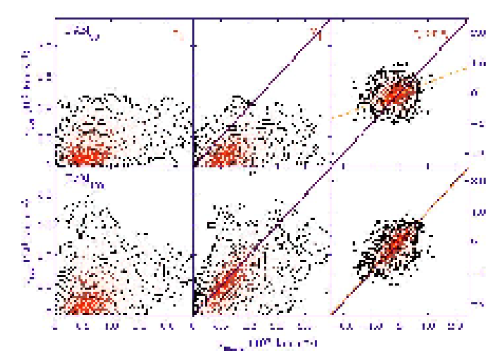
Figure 10: Point-to-point comparison (scatter plot) of FAM velocity decompositions wrt. the corresponding $N$-body velocity of the involved $\Lambda$CDM mock sample. Both the parallel projection $v_{\parallel}$ (centre frames) as well as the perpendicular projection $v_{\perp}$ along the $N$-body velocity direction are analyzed. Top row: FAM₃₀ reconstruction against $N$-body velocity equivalent. Bottom row: FAM₁₀₀ reconstruction against $N$-body velocity equivalent. Lefthand column: $v_{\parallel}$. Central column: $v_{\perp}$. Righthand column: The $x$ component of the velocity, $v_{x}$. The solid line in the righthand column frames indicates the identity line $v_{x,FAM}=v_{x,N-body}$. The dashed line indicates the best linear fit. Evidently, the FAM₃₀ deviate systematically from the identity line. The point scatter density is characterized by the contours, indicating iso-density surfaces. See Table 3.

A straightforward comparison is that between the Cartesian velocity components $v_{i}$ of the FAM reconstructed velocities and the $N$-body velocities (Fig 10, righthand column). Complementary regressions involve coordinate system independent aspects of galaxy velocities. These involve the velocity amplitude $|v_{\scriptstyle{\rm FAM}}|$ (Fig. 9, top lefthand panel), the component of each FAM velocity parallel to the corresponding $N$-body velocity, $v_{\parallel}$ ($\equiv$ v_proj), and the additional perpendicular component $v_{\perp}$ (Fig 10, first column). Misalignments between the real $N$-body velocity and the FAM velocity reconstructions should indicate in how far a reconstruction has been failing to take into account all relevant gravitational forces along the path of a particle. Systematic misalignments reveal themselves in the scatter diagram of the angle $\theta$ between the FAM velocity and the galaxies’ $N$-body velocity ${\bf v}_{\scriptstyle{\rm Nbody}}$ (in Fig. 9 we plot $\mu\equiv\cos(\theta)$, bottom righthand panel). In terms of the character and systematics of the underlying physics and dynamics the residual velocities, [$N$-body - FAM], represent highly informative aspects in our analysis. They are assessed in (Fig. 9, top righthand panel) and Figure 11.

The significance and strength of correlations between the $N$-body and FAM velocity components in the scatter diagrams are analyzed by means of a linear regression and correlation analysis. To circumvent excessive pollution of the computed parameters by the virialized motions in high-density regions (see sect. 3.3), the galaxy velocity components in these regression analyses involve $2h^{-1}{\rm Mpc}$ tophat filtered velocity fields. The resulting numerical values of the correlation parameters are listed in Table 3. Table 3 is organized in two separate sections, one for the regression analysis results of the $\Lambda$CDM mock samples (top section) $\tau$CDM samples (bottom section). For both the $\Lambda$CDM and the $\tau$CDM section we list the results for four velocity related quantities, each separately for the FAM₃₀ and the FAM₁₀₀ reconstructions.

The presence of significant correlations between FAM reconstructions and their $N$-body counterparts is evaluated on the basis of the nonparametric Spearman correlation coefficient $R_{Spear}$. The linear regression parameter $R_{lin}$ quantifies the linearity of the relation. Prevailing in most situations, the linear regression parameters are used to characterize the relation between reconstructed and real $N$-body velocities: the zero-point (offset) $a_{0}$, the slope $a_{lrg}$ and the dispersion $\sigma_{lrg}$ around the linear regression relation. We assume equal errors in FAM and $N$-body velocities, as both are affected by similar shot noise errors (while $2h^{-1}{\rm Mpc}$ top hat smoothing significantly reduces the impact of virial motions on FAM velocity predictions). In addition, we also list the rms scatter of the parameters, estimated on the basis of the results for the 10 different mock catalogs (for each of the four different configurations).

7.3 Inventory

7.3.1 Velocity Amplitude

In the top lefthand frame of Fig. 9 the FAM₃₀ and FAM₁₀₀ velocity amplitudes are compared with their $N$-body counterpart $|v_{\scriptstyle{\rm Nbody}}|$. The FAM₃₀ diagram differs considerably from the FAM₁₀₀ diagram: the FAM₃₀ velocities are systematically smaller than their FAM₁₀₀ counterparts. Also, while the latter have a strong one-to-one correlation to the $N$-body velocities, the FAM₃₀ diagram shows a systematic offset with respect to this relation (the solid line) and a somewhat larger scatter.

While the FAM₁₀₀ diagram tapers out to higher velocities and even shows a few points with $|v_{\scriptstyle{\rm FAM}}|>2000\ {\rm km\leavevmode\nobreak\ s^{-1}}$, there is a firm ceiling of $|v_{\scriptstyle{\rm FAM}}|\approx 1300\ {\rm km\leavevmode\nobreak\ s^{-1}}$ for the FAM₃₀ velocities. It is a direct reflection of the FAM₃₀ reconstructions missing out on the gravitational force contributions by the external mass distribution. The asymmetric nature of the scatter in both diagrams is due to particles in high density regions.

To a good approximation, the correlation between the FAM₁₀₀ velocity amplitudes and $|v_{\scriptstyle{\rm Nbody}}|$ is that of a linear identity relation: the solid line, $|v_{\scriptstyle{\rm Nbody}}|=|v_{\scriptstyle{\rm FAM}}|$, forms a good fit to the scatter diagram (see Table 3: $a_{lrg}\rightarrow 1$). The significantly higher value of Spearman’s correlation coefficient (Table 3: $R_{Spear}\approx 0.68$ vs. $R_{Spear}\approx 0.54$ for FAM₃₀) indicates and confirms the visual impression of Fig. 8) of the tight correspondence between the FAM₁₀₀ and $N$-body vector velocity fields. The FAM₃₀ results stand in marked contrast: the majority of the FAM₃₀ velocities have a systematically lower amplitude than their $N$-body counterparts. It results in a relation with a significantly shallower slope than that of the identity relation $|v_{\scriptstyle{\rm Nbody}}|=|v_{\scriptstyle{\rm FAM}}|$ (also see table 3): objects with a higher velocity have a larger discrepancy. The contribution by the missing large-scale velocity component ${\bf v}_{\rm lss}$ to the amplitude of the FAM velocity includes a cross-term ($-{\bf v}_{\rm Nbody}\cdot{\bf v}_{\rm lss}$), a term dependent on the velocity ${\bf v}_{\rm Nbody}$ of the galaxy. Most of the missing large-scale velocity component ${\bf v}_{\rm lss}$ is due to the absence of a bulk flow term in the FAM₃₀ reconstructions. Subtle and/or higher order external gravitational effects play an additional role: the velocity vector diagrams did already reveal that the presence of shear should be one of the main contributors (cf. eq. 21).

When comparing the $\Lambda$CDM FAM velocity amplitudes with those of the $\tau$CDM reconstructions it is evident that in the case of the FAM₃₀ reconstructions the latter adhere considerably better to the corresponding $N$-body values. The linear fitting slope $a_{lrg}$ (see table 3) is considerably closer to unity for the $\tau$CDM samples than for the $\Lambda$CDM samples. Over a 30$h^{-1}{\rm Mpc}$ volume the external density inhomogeneities in the $\Lambda$CDM cosmology will induce considerably higher bulk flows than the more moderate $\tau$CDM perturbations, which is entirely in line with the theoretical expectation (fig 2). In the case of the FAM₁₀₀ reconstructions the qualitative differences are far less prominent. On the scale of $\sim 100h^{-1}{\rm Mpc}$ the mass distribution in both the $\tau$CDM and $\Lambda$CDM simulation volumes have converged to homogeneity and no major bulk flows are to be expected.

7.3.2 Velocity Decompositions

In the two righthand frames of Fig. 10 we show the scatter diagrams for the x-component of the FAM₃₀ (top) and FAM₁₀₀ velocities (bottom). Although with a significant level of scatter, the FAM₁₀₀ diagram can be fitted quite well by a straight line with a slope close to unity (linear regression line: dashed,unity line: solid). That the equivalent FAM₃₀ diagram may also be fitted by a straight line, be it with a slope significantly smaller than unity is not entirely straightforward. It stems from an intricate interplay between the small scale velocity field and its larger scale contributions, which in most circumstances are not uncorrelated (Berlind, Narayanan & Weinberg bernarw2000 (2000)).

Table 3 lists the linear regression parameters. Although the average best fitting slopes for the FAM₁₀₀ velocities are either larger ($\tau$CDM) or smaller ($\Lambda$CDM) than unity, the deviation from unity is considerably smaller than that for the FAM₃₀ velocities, well within the $\sim 1\sigma$ uncertainty interval. In all, these regression results do adhere to the expected and noted trend of FAM₁₀₀ velocities accounting for practically all contributions to the local velocity field and FAM₃₀ velocities systematically neglecting significant external contributions. Notice that the scatter around the regression lines for the FAM₃₀ and FAM₁₀₀ reconstructions is of comparable magnitude (as may be inferred from the superposed number density contours).

While the choice of any Cartesian coordinate system is an arbitrary one we have also addressed the decomposition of the particle velocities in one defined by the system itself. The FAM velocities are decomposed in a component projected along the corresponding $N$-body velocity, $v_{proj}$ (or $v_{\parallel}$) and the complementary perpendicular component, $v_{\perp}$. The second column of figure 10 contains the scatter diagrams for the parallel component of the FAM₃₀ (top) and FAM₁₀₀ (low) velocities. Qualitatively, the behaviour of both diagrams resembles that of the velocity amplitude scatter diagrams in fig. 9. A $1-1$ relation between FAM₁₀₀ velocities and $N$-body velocity amplitude represents a reasonable fit (solid line: slope $a_{lrg}\approx 0.99$). The FAM₃₀ diagram not only appears to deviate strongly from such a $1-1$ relation, it may even fail to fit any linear relation. Also, none of the projected FAM₃₀ velocity components appears to supersede a value of $\approx 1200\ {\rm km\leavevmode\nobreak\ s^{-1}}$. Given the fact that the equivalent FAM₁₀₀ component even surpasses values of $\approx 2000\ {\rm km\leavevmode\nobreak\ s^{-1}}$, this confirms the systematic deficiency of the gravitational field in the FAM₃₀ evaluations.

From the scatter diagrams for the perpendicular FAM velocity components, $v_{\perp}$, one can infer that almost all systematic effects are confined to the parallel components $v_{\parallel}$. For both FAM₃₀ and FAM₁₀₀ the complementary perpendicular component lacks a systematic correlation with the $N$-body velocity. It mainly represents unrelated scatter, with a magnitude concentrated around values of $\sim 200-250\ {\rm km\leavevmode\nobreak\ s^{-1}}$. The only difference between the FAM₃₀ and FAM₁₀₀ reconstructions is that for the latter $v_{\perp}$ involves considerably higher values, reflecting the higher amplitude of the FAM₁₀₀ velocities. FAM₃₀ velocities, on the other hand, involve stronger misalignments (section 7.3.3).

7.3.3 Velocity Alignments

Misalignments between the reconstructed FAM velocities and the $N$-body velocity vectors are the result of a few effects. A major source is that of localized small-scale effects. These are not expected to lead to systematic offsets: they will have a noisy character and reflect random motions in highly nonlinear environments, in particular those of dense virialized regions. Because these have no preferred direction, they behave like randomly oriented “residual” velocities wrt. to the real $N$-body velocities of galaxies. Of an entirely different nature are misalignments stemming from the systematic neglect of the external gravitational forces. Because the resulting residual velocity vectors comprise systematic components along one or a few preferred directions, a distinctly anisotropic distribution is the result. This reflect itself as a systematic trend for total $N$-body galaxy velocities to be aligned along the residual velocity components.

For both the FAM₃₀ and FAM₁₀₀ reconstructions we computed the angles between the $N$-body velocity vector and the FAM velocities. The lower righthand panel in Figure 9 confirms that the alignments of “residuals” and total velocity is indeed considerably stronger for the FAM₃₀ reconstructions than the FAM₁₀₀ ones. The figure plots, for each galaxy in the sample, the misalignment angle $\theta$ (or, rather, $\mu=\cos(\theta)$) versus the $N$-body velocity magnitude $v_{\scriptstyle{\rm Nbody}}$. For the FAM₁₀₀ velocities we see a near isotropic distribution of angles. With the exception of a minor concentration near perfect alignment, $\cos(\theta)=1$, the distribution is sweeping out nearly uniformly over the full range of $\mu\equiv\cos(\theta)=1\rightarrow-1$. If at all there is a trend in velocity amplitude, it appears to be the weak tendency for large velocities to be better aligned.

The above results reflect the observation that FAM₁₀₀ residual velocities do mainly consist of small-scale random effects. The FAM₃₀ residuals form a telling contrast. They are heavily aligned along the full $N$-body velocities, with a very strong concentration near $\theta=0$. Although occasionally there are serious misalignments, their occurrence diminishes rapidly towards large $\theta$. When they occur it almost exclusively concerns small velocities, mostly corresponding to serious misalignments between the locally induced velocity and the added external velocity component.

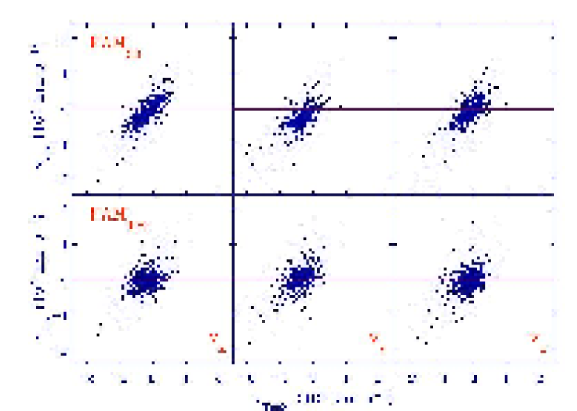
Figure 11: point-to-point comparison (scatter plot) of the Cartesian components of the residual velocity ${\bf v}_{FAM}-{\bf v}_{Nbody}$ components against corresponding $N$-body velocity ${\bf v}_{Nbody}$. From left to right: $v_{x}$, $v_{y}$ and $v_{z}$. Top row: FAM₃₀ reconstructed velocity. Bottom row: FAM₁₀₀ reconstructed velocity.

7.3.4 Velocity Residuals

The residuals accumulate all systematic physical effects as well as random artifacts. They are therefore an excellent source of information on the dynamical role of matter concentrations in the various galaxy sample volumes. If there are large external contributions to the galaxies’ velocity these will constitute a major part of the residuals. On the other hand, if most of those influences are contained within the sample volume treated by FAM, the residuals may mainly reflect localized nonlinearities and artifacts of the FAM method. Scatter diagrams involving the residual velocities will indicate systematic trends and are well suited for elucidating the character and underlying dynamics of external influences.

Figure 11 elaborates on this observation. In two successive rows, the top one for the FAM₃₀ reconstructions and the bottom one for the FAM₁₀₀ reconstructions, it displays the residuals ${\bf v}_{res}$ for each of the three Cartesian velocity components, $v_{x}$, $v_{y}$ and $v_{z}$. Each panel plots the velocity component residual as a function of the corresponding $N$-body velocity component.

The mark of a bulk velocity is a constant offset of the scatter diagram, a translation of all FAM velocities by a constant term. This is indeed what is observed in the FAM₃₀ $v_{y}$ scatter diagram: the vast majority of points is located beneath the $v_{y}=0\leavevmode\nobreak\ \ {\rm km\leavevmode\nobreak\ s^{-1}Mpc^{-1}}$ line. It is a telling confirmation of the impression yielded by the corresponding velocity vector fields in Fig. 7. The velocity vector field revealed the presence of strong bulk flow oriented almost perfectly along the $y$-axis: clearly visible in the $N$-body velocity field, hardly present in the corresponding FAM₃₀ velocity field, and representing a major component of the residual field [$N$-body - FAM₃₀]. When turning to the equivalent FAM₁₀₀ diagram, the indicative offset for a bulk flow has almost completely disappeared. This implies that the source(s) for the bulk flow should be found within the region between $30h^{-1}{\rm Mpc}$ and $100h^{-1}{\rm Mpc}$. The equivalent $v_{x}$ and $v_{z}$ FAM₃₀ residual scatter diagrams do confirm the visual impression of there hardly being a bulk flow contribution along the $x$- and $y$-directions.

Additional systematic behaviour is readily apparent in Fig 11: the diagrams show an almost linear increase of residual velocity with $N$-body velocity. Also, we find that the $v_{x}$ scatter is skewed towards negative $v_{res}$ values while the $v_{z}$ diagram is skewed towards positive $v_{res}$ values. In the equivalent FAM₁₀₀ scatter diagrams the linear increase of $v_{res}$ and the asymmetry in the $v_{x}$ and $v_{z}$ diagram has almost disappeared: the dense core of points has turned into a compact and nearly horizontal bar symmetrically distributed around the $v_{res}=0\ {\rm km\leavevmode\nobreak\ s^{-1}}$ line. To a large extent this is explained by the much smaller contribution of external tidal shear to the flows over $100h^{-1}{\rm Mpc}$ volumes (cf. Fig. 2).

The mark for external shear is a near linear increase of residual velocities as a function of their $N$-body (or measured) velocity. Depending on the location ${\bf x}$ of a galaxy within the sample volume and with respect to the shear configuration its participation in a shear flow will involve a velocity component $v_{s}\equiv\sum s_{ij}x_{j}$. This may involve a negative or a positive contribution. With such shear contributions representing a non negligible component to the total velocity, its systematic contribution to a largely random local residual signal reshuffles the velocities such that on average the largest velocity involves the largest residual contribution.

With prominent large-scale bulk and shear motions at large, the FAM₁₀₀ residual scatter diagram has largely transformed into a featureless and purely random point distribution. The residuals mainly involve uncorrelated small-scale effects and are nearly independent of the amplitude of the $N$-body velocity. Some additional artifacts are seen upon closer inspection: the presence of diffuse “S”-shaped point clouds in both the FAM₃₀ and FAM₁₀₀ residual diagrams, tapering off towards a steep tail at both the negative and positive side of the plots.

The corresponding scatter diagrams for the velocity residual amplitudes $|{\bf v}_{\scriptstyle{\rm res}}|=|{\bf v}_{\scriptstyle{\rm FAM}}-{\bf v}_{\scriptstyle{\rm Nbody}}|$ represents a summary of the systematic trends (Fig. 10). The FAM₃₀ velocity residuals show a near linear increase as a function of the $N$-body velocity, starting with an offset, indicative of the ingredients of bulk and shear flow in the residuals. The lack of any clear correlation between $|{\bf v}_{\scriptstyle{\rm res}}|$ and $|{\bf v}_{\scriptstyle{\rm Nbody}}|$ in the case of the FAM₁₀₀ residuals confirms the absence of such systematic components. More clearly than in the case of the individual Cartesian components, the presence of local nonlinear motions may be discerned from the extensive surrounding clouds of outliers.

7.4 Power Spectrum Dependence

The contrast between FAM₃₀ and FAM₁₀₀ scatter diagrams is more pronounced in the case of the $\Lambda$CDM mock catalogs than in those assembled for the $\tau$CDM universes. This clearly reflects the fact that within the $\Lambda$CDM scenario cosmic structure is characterized by a larger coherence scale. It implies the presence of larger and more coherent structures whose size exceeds $30h^{-1}{\rm Mpc}$. Their combined gravitation impact will yield a stronger systematic impact in the velocity-velocity comparisons. On the other hand, the dispersions listed in table 3 also show that it would hardly be possible to infer information on the cosmological scenario on the basis of one individual realization. The large dispersion around the average slopes, in particular in the case of the $\Lambda$CDM Universe, show that the magnitude of the external dynamical effects may vary appreciably as a function of the location of the (mock) NBG sample within the simulation box. Local measurements will therefore be unable to separate cosmological effects from those stemming from local variations.

7.5 Nonlinearities

The point-to-point diagrams discussed above all contain a substantial level of scatter around the inferred regression relations. With a few exceptions the scatter of velocity quantities is in the order of $\sim 200-250\ {\rm km\leavevmode\nobreak\ s^{-1}}$, for both the $\Lambda$CDM as well as the $\tau$CDM FAM reconstructions. The main source for this scatter are the virial motions in the high density and mildly nonlinear environments. Also shot noise provides a substantial additional contribution. In the case of small filter radii, another source of scatter is formed by spurious very close pairs of points in the parent $N$-body catalog which for artificial reasons failed to collapse into a single object (Branchini, Eldar & Nusser branchini02 (2002)). Scatter may also be due to higher order multipole components in the external gravity field. An inspection of the particle configurations and the velocity vector maps does unmistakably show significant systematic variations on top of dipolar and quadrupolar components. However, tests restricting the analysis to points in the central regions of the sample produced no substantial decrease in level of scatter. This seems to argue for a minor role of such contributions.

8 Bulk Flow and Tidal Shear:
     Velocity Flow Multipole Components

In the previous sections we have found that in order to obtain a good representation of the local cosmic velocity field it is necessary to take into account the external gravitational influence. This was accomplished through the incorporation of the fully detailed external mass distribution contained in the (flux-limited) galaxy catalogs. This involved the galaxy distribution out to distances of $100h^{-1}{\rm Mpc}$. The reconstructions showed that modelling of velocity fields by FAM with the inclusion of matter concentrations on such large scales is indeed rewarding.

In nearly all situations where the local volume $V_{int}$ is suitably large, the small-scale details of the external mass configuration are rather irrelevant for constructing an appropriate model of the flows in the local Universe. An appropriate approximate expression for the the gravitational potential $\Phi_{ext}({\bf r})$ inside the internal volume $V_{int}$ due to the surrounding external matter distribution follows from its expansion in multipole contributions. Assuming a spherical local volume with radius $R_{int}$, the potential $\Phi_{ext}$ may be written in terms of a multipole expansion of spherical harmonics $Y_{lm}(\theta,\phi)$ (see e.g. Jackson jackson (1975))

$$\Phi_{ext}({\bf r}) \,=\, -\,\int_{R_{int}}^{\infty}\,{\displaystyle G\rho({\bf x}^{\prime})\over\displaystyle|{\bf x}-{\bf x}^{\prime}|}\,d{\bf x}^{\prime}$$

$$\,=\, -\,\sum_{l=0}^{\infty}\,\sum_{m=-l}^{m=l}\,{\displaystyle 4\pi G\over\displaystyle 2l+1}\,{\cal Q}_{lm}\,Y_{lm}(\theta,\phi)\,r^{l}\,,$$

in which the multipole moments ${\cal Q}_{lm}$ relate to the external density field $\rho({\bf x}^{\prime})$ as

$${\cal Q}_{lm}\,=\,\int_{r}^{\infty}\,\rho({\bf x}^{\prime})\,r^{\prime l-3}\,Y_{lm}^{*}(\theta^{\prime},\phi^{\prime})\,d{\bf x}^{\prime}\,.\\$$ (23)

Most contributions to the external gravity ${\bf g}_{ext}$ will be confined to these dipole and quadrupole components, induced by the corresponding large-scale constellations in which the surrounding matter concentrations have grouped themselves. Here we will assess the approximation in which the potential expansion (eqn. 8) is restricted to the monopole term $l=0$, the dipole term $l=1$ and the quadrupole term $l=2$,

$$\Phi_{ext}({\bf r})\,\approx\,\Phi_{0}({\bf r})\,+\,\Phi_{1}({\bf r})\,+\,\Phi_{2}({\bf r})\\$$

with

$$\Phi_{l}({\bf r})\,=\,-\,\sum_{m=-l}^{m=l}\,{\displaystyle 4\pi G\over\displaystyle 2l+1}\,{\cal Q}_{lm}\,Y_{lm}(\theta,\phi)\,r^{l}\,.$$ (24)

To explore the nature of the external component in the total gravitational field in the Local Universe we proceed by probing it through the resulting peculiar velocity field. The amplitude of higher order terms may be assumed to be so small that one cannot expect to deduce any significant value, given the sizeable errors in the available galaxy peculiar velocity datasets, we may expect this to be a reasonable approximation. We investigate the velocity field by decomposing the residual velocity field – i.e. the component in the velocity field which could not be accounted for in the FAM₃₀ reconstruction and supposedly induced by external influences – into its multipole components. Once we have determined the bulk flow component and shear tensor components in the tidal velocity field, we will assess whether we can indeed relate this to the external gravitational (“tidal”) influence within the local Universe.

Restricting the description of the external gravitational influence to the first few orders of its multipole expansion has several advantages. The large-scale external dipole and quadrupole gravity perturbations retain a largely linear character, simplifying the velocity field analysis and thus retaining the direct linear relation between gravity and velocity field. Also, by discarding its small-scale fluctuating contributions a physically more transparent image of the velocity field is obtained. This allows a straightforward relation and translation towards the corresponding large-scale pattern of the surrounding mass distribution. A final practical issue of some importance is the fact that the dipole and quadrupole characterization is particularly suited for an implementation in FAM. Restricting the external force field to these moments alleviates the need to take into account a large sample of external galaxies. Not only is the latter computationally expensive, in practice it is even not always feasible.

8.1 Velocity Field Multipole Decomposition

In the multipole analysis we restrict ourselves to the externally induced velocity components, ${\bf v}_{ext}$, which in the following we frequently designate by the term “tidal”. For each object, the “tidal” velocity vector is determined by subtracting the internally induced velocity field, ${\bf v}_{int}$, from the object’s full velocity. The latter is usually the $N$-body velocity of the mock galaxy, although we will assess the possibility of using the FAM₁₀₀ velocity as a reasonable alternative. The internal velocity ${\bf v}_{int}$ is deduced by evaluating, through our FAM computations, the impact of the internal matter distribution within the internal catalog volume $V_{int}$. The resulting (residual) peculiar velocity vector ${\bf v}_{ext}$ field may then be expressed in terms of a Taylor series description as function of spatial position ${\bf x}$.

For the practical implementation, we follow the general scheme described by Kaiser (kaiser (1991)). The velocity field Taylor expansion is truncated at the quadratic term and is restricted to the dipole and quadrupole moments (and a minor monopole term). The tidal velocity field ${\bf v}_{ext}$, is then modeled by the the first two components, a bulk flow vector, ${\tilde{u}}_{i}$, and a quadratic shear tensor contribution, ${\tilde{s}}_{ij}$,

$$v_{ext,i}={\tilde{u}}_{i}+{\tilde{s}}_{ij}x\hat{x}_{j},\qquad{\rm where}\qquad i,j=\{1,2,3\}\ ,$$ (25)

in which $i,j$ denotes the Cartesian component indices. As in eqn. 21, the vectors $\hat{x}_{j}$ represent the vector components along the Cartesian $j$ direction of the spatial unity vector oriented along the object position vector ${\bf x}$. Using these notations, we can easily reconfigure eqn. 25 and express the $i$-component of the velocity of object $n$ into a product of the vectors $F_{n,I}$ and $V_{Ii}$,

$$v_{n,i}=\sum_{I=1}^{4}F_{n,I}({\bf x})V_{Ii}$$

Field	Cosmology	$v_{bulk}$	$s$	$s_{1}$	$s_{2}$	$s_{3}$
Configuration		(km s-1)
	$\Lambda$CDM	313  $\pm$ 65	13.3  $\pm$ 3.8	8.8  $\pm$ 3.6	0.6  $\pm$ 2.5	-9.4  $\pm$ 2.3	(km s-1 Mpc-1)
	$\tau$CDM	216  $\pm$ 57	13.6  $\pm$ 4.6	8.9  $\pm$ 3.1	1.1  $\pm$ 2.0	-10.0  $\pm$ 3.7
$N-$body – FAM30
	$\Lambda$CDM		399  $\pm$ 115	264  $\pm$ 107	19  $\pm$   76	-283  $\pm$   70	(km s-1)
	$\tau$CDM		409  $\pm$ 137	267  $\pm$   92	33  $\pm$   60	-300  $\pm$ 110
	$\Lambda$CDM	81  $\pm$ 51	3.7  $\pm$ 1.2	2.6  $\pm$ 0.9	-0.2  $\pm$ 0.8	-2.4  $\pm$ 1.0	(km s-1 Mpc-1)
	$\tau$CDM	121  $\pm$ 54	4.8  $\pm$ 1.1	3.4  $\pm$ 1.0	0.0  $\pm$ 0.8	-3.3  $\pm$ 0.8
$N-$body – FAM100
	$\Lambda$CDM		110  $\pm$ 36	78  $\pm$   27	-6  $\pm$ 25	-72  $\pm$   30	(km s-1)
	$\tau$CDM		145  $\pm$ 33	101  $\pm$  30	-1  $\pm$ 23	-100  $\pm$  23
	$\Lambda$CDM	317  $\pm$ 89	14.0  $\pm$ 4.6	9.4  $\pm$ 4.0	0.5  $\pm$ 2.9	-9.9  $\pm$ 3.0	(km s-1 Mpc-1)
	$\tau$CDM	245  $\pm$ 60	15.3  $\pm$ 4.3	9.8  $\pm$ 2.5	1.4  $\pm$ 2.9	-11.2  $\pm$ 3.8
FAM100 – FAM30
	$\Lambda$CDM		421  $\pm$ 138	281  $\pm$ 120	15  $\pm$  86	-296  $\pm$   91	(km s-1)
	$\tau$CDM		458  $\pm$ 128	293  $\pm$   75	42  $\pm$  87	-335  $\pm$ 115
	$\Lambda$CDM	81  $\pm$ 51	2.4  $\pm$ 1.3	-0.6  $\pm$ 1.7	-0.2  $\pm$ 1.4	0.9  $\pm$ 1.3	(km s-1 Mpc-1)
$N-$body - FAMmpl
	$\tau$CDM	121  $\pm$ 54	2.9  $\pm$ 0.8	-0.6  $\pm$ 1.6	-0.5  $\pm$ 1.6	0.9  $\pm$ 1.7

Table 4: Average results for the tidal bulk amplitude and shear eigenvalues. The errors represent the $1\sigma$ scatter around the average value. Col. 1: Tidal field region where the velocity components were computed. The first two sections refer to the tidal field computed from the $N$-body – FAM models. In the third section the external tidal influences are determined by the large region modeled on FAM₁₀₀ instead of the $N-$body samples. The fourth region refers to the residual field between $N-$body and FAM_mpl after the external contributions have been accounted for in the FAM modeling: FAM₃₀ + tidal bulk + tidal shear (see text sec. 8.2 and sec. 8.5 for details). Col. 2: Cosmological model. Col: 3: bulk flow, $v_{bulk}$. Col: 4: shear eigenvalue amplitude, $|s|$. Col: 5: $s_{1}$ eigenvalue (stretching). Col. 6: $s_{2}$ eigenvalue (middle). Col. 7: $s_{3}$ eigenvalue (compressional).

Figure 12: Velocity Field Multipole Decomposition: the total $N$-body velocity field, involving the same one as in Fig. 13 and Fig. 14, decomposed into its four different components. The coordinate system is that defined by the tidal shear tensor, see Fig. 13. At each row we depict the velocities in the $(x-y)$, $(x-z)$ and $(y-z)$ plane. Top: the locally induced velocity, approximated by the FAM₃₀ realization. Second row: the monopole component, a result of the slight local expansion due to its underdensity wrt. the global Universe. Third row: the bulk flow, of which most is concentrated in the $(x-y)$ and $(y-z)$ plane. Fourth row: the shear flow component.

in which the data 4-vector $F_{I}$ and the velocity field component 4-vector $V_{Ii}$ are defined as

$$F_{n,I} = \{1,x\hat{x}_{1},x\hat{x}_{2},x\hat{x}_{3}\}$$

$$V_{Ii} = \{{\tilde{u}}_{i},{\tilde{s}}_{i1},{\tilde{s}}_{i2},{\tilde{s}}_{i3}\}\ .$$ (26)

The “dipolar” bulk flow components ${\tilde{u}}_{i}$ and “quadrupolar” velocity shear components ${\tilde{s}}_{ij}$ can then be obtained by solving for the vectors $V_{Ii}$ on the basis of a fitting analysis (to be precise, ${\tilde{s}}_{ij}$ also includes a minor residual “monopole” expansion/contraction term). We accomplish this by computing for each Cartesian component $i$ the values for the multipole elements ${\tilde{u}}_{i}$ and ${\tilde{s}}_{ij}$ which minimize $\chi^{2}$

$$\chi^{2}=\sum_{n=1}^{N_{objs}}\Big{(}v_{n,ext,i}-\sum_{I}F_{n,I}({\bf x})V_{Ii}\Big{)}^{2}\ ,$$ (27)

to be evaluated on the basis of the data sample of $N_{obj}$ objects at locations ${\bf x}_{n}$ and with inferred “external” velocities ${\bf v}_{n,ext}$. The bulk flow and velocity shear in the externally induced velocity component ${\bf v}_{ext}$, along with a residual expansion term,

$$v_{ext,i}\,\approx\,v_{exp,i}+v_{bulk,i}\,+\,v_{shear,i}$$ (28)

will follow directly from the inferred values of the 4-vector components $V_{Ii}$:

$$v_{exp,i} \,=\, {1\over 3}\,Tr({\tilde{s}})\,x\hat{x}_{i}$$

$$v_{bulk,i} \,=\, {\tilde{u}}_{i}\,;\qquad\qquad v_{shear,i}\,=\,\sum_{j=1}^{3}\,{\tilde{s}^{\prime}}_{ij}x\hat{x}_{j}$$ (29)

in which $Tr(s)$ is the trace of the tensor $s_{ij}$ and ${\tilde{s}^{\prime}}_{ij}$ the traceless shear tensor

$$Tr({\tilde{s}}) \,\equiv\, {\tilde{s}}_{11}+{\tilde{s}}_{22}+{\tilde{s}}_{33}$$

$${\tilde{s}^{\prime}}_{ij} \,=\, {\tilde{s}}_{ij}-{1\over 3}Tr({\tilde{s}})\,\delta_{ij}\,.$$ (30)

8.2 Velocity Multipole Analysis: results

The results of our analysis are summarized in Table 4. It lists the average quantities for the tidal bulk flow and shear components for the two cosmological scenarios discussed in this work. The table has been organized in four (horizontal) sections. Each corresponds to another “differential” velocity field, the difference between two differently processed velocity fields.

For both the $\Lambda$CDM and the $\tau$CDM model each of the quoted values in Table 4 involve the average and standard deviation determined on the basis of ten different realizations. This adds up to 8 configurations, two cosmologies per section. For each of the 8 configurations, in the third column the table lists the dipole component of the external velocity field, the bulk flow $v_{bulk}$. Subsequently, the velocity shear is specified in terms of the three eigenvalues $s_{1}$, $s_{2}$ and $s_{3}$ of the traceless shear tensor. This is preceded in the fourth column by the amplitude $s$ of the shear. Note that shear is quoted in two units. First, units of $\ {\rm km\leavevmode\nobreak\ s^{-1}Mpc^{-1}}$, followed by the equivalent velocity differential in $\ {\rm km\leavevmode\nobreak\ s^{-1}}$ over a volume of $30h^{-1}{\rm Mpc}$ radius. The intention of the latter is to offer a directly appreciable comparison between the relative importance of bulk flow and shear contributions.

Each of the four sections specifies the values of the computed dipole and quadrupole moments of the velocity field of the corresponding sample. The first section relates to a multipole analysis of the differential velocity field between the full $N$-body velocity field and the FAM₃₀ velocity reconstructions of the inner $30h^{-1}{\rm Mpc}$ region, $N$-body - FAM₃₀. The resulting residual velocity field has been generated by the mass distribution beyond a radius of $30h^{-1}{\rm Mpc}$. On these linear scales the inferred dipole and quadrupole components of the velocity field may be directly related to the moments of the surrounding mass distribution.

The second section of Table 4 does the same for the larger $100h^{-1}{\rm Mpc}$ region. The outcome of similar analyses are presented in the third and fourth section. The third section repeats the analysis of the first section, except that the external tidal influences are determined on the basis of the difference between the FAM velocity reconstructions within the large $100h^{-1}{\rm Mpc}$ region and the inner $30h^{-1}{\rm Mpc}$ region. Earlier, in Section 6.3, we have found that the major share of the origin of the external tidal field is confined to this region and that it therefore may well be determined from the residuals between FAM₁₀₀ and FAM₃₀. The comparison between the inferred multipole moments of the velocity differences between FAM₁₀₀-FAM₃₀ in the third section and those in the first section are therefore expected to be rather similar, any systematic differences originating in tidal effects generated beyond a radius of $100h^{-1}{\rm Mpc}$. The fourth section in Table 4 refers to the values of the residual tidal velocity field between $N$-body – FAM_mpl, the FAM sample after having accounted for the missing external tidal contributions, FAM₃₀ + tidal bulk + tidal shear (see sec. 8.5). If indeed all significant contributions can be characterized by their dipolar and quadrupolar contributions, the multipole values in this section are expected to be negligible.

8.3 Velocity Multipole Contributions: Maps

For a direct visual appreciation of the various multipole contributions to the tidal velocity field we assess the “tidal” velocity field $N$-body - FAM₃₀, the velocity field generated by the mass distribution beyond a radius of $30h^{-1}{\rm Mpc}$, for one of the $\Lambda$CDM catalogs. The presented maps concern the same $\Lambda$CDM catalog as those presented in the maps of Figures 7. The map of the projection of this “tidal” velocity flow onto three central planes is shown in the top row of Figure 13.

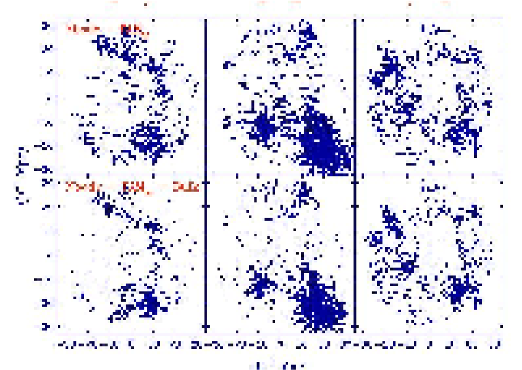
Figure 13: 2D projected peculiar (residual) velocities for the same mock catalog as in Fig. 7 and Fig. 8 in three perpendicular central planes of $10h^{-1}{\rm Mpc}$ width. The coordinate frame is rotated such that the bulk flow velocity is oriented along the $x$-direction. Within the plane perpendicular to the $x$-axis, the $y$ and $z$ axes are chosen arbitrarily. First row: the residual velocity (ie. tidal velocity) $N-$body - FAM₃₀. Second row: residual velocities after subtraction bulk flow component. The resulting residual field is clearly dominated by a shear pattern, most notably in the $y-z$ plane.

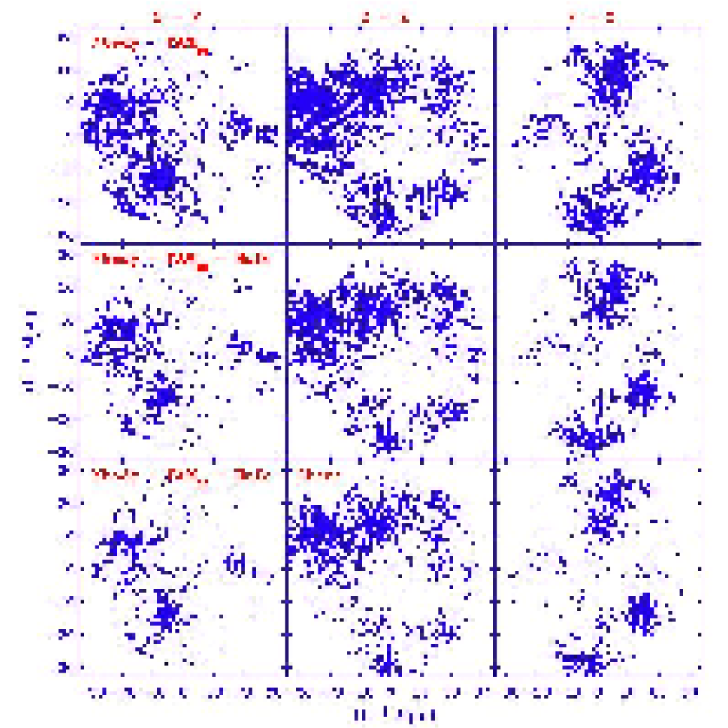
Figure 14: 2D projected peculiar velocities for the same mock catalog as in Fig. 7 and Fig. 8 in three perpendicular central planes of $10h^{-1}{\rm Mpc}$ width. The coordinate frame is defined by the three eigenvectors of the shear tensor. The $x$-axis is aligned along the direction of the largest (stretching) eigenvalue, the $y$-axis is aligned along the middle eigenvalue and the $z$-axis along the smallest (compressional) eigenvalue. The first two rows are the same as Fig. 13, within the “shear reference system”. The third row depicts the final residual field after subtraction of the quadrupolar shear component.

8.3.1 Dipolar component: bulk flow

The externally generated velocity flow is dominated by its bulk flow component. This is in general true for both cosmologies. The large impact of the bulk flow over the local 30$h^{-1}{\rm Mpc}$ volume can be immediately inferred from the values in the first section of Table 4, revealing contributions in excess of $200\ {\rm km\leavevmode\nobreak\ s^{-1}}$.

To facilitate visual appreciation of this observation we have have reoriented the reference system in Figure 13 such that the $x$-axis is oriented along the bulk flow. While the original Cartesian system is an arbitrary one and thus lacks a physical context, the “bulk flow reference system” confines the inferred bulk flow ${\tilde{u}}$ exclusively to the $x$-direction. As a result there are no bulk flow components in the corresponding $y$- and $z$-direction (note that within the $y-z$ plane their direction is arbitrarily defined). The pre-eminence of the bulk flow component can be immediately seen in the $x-y$ and $x-z$ frames in the top row of Figure 13. Note that the same velocity maps, mostly so the $y-z$ frame, reveal a clear shear pattern.

8.3.2 Quadrupolar component: velocity shear

Seeking to assess the quadrupolar term in the external velocity field we first remove the remaining expansion term from ${\tilde{s}}_{ij}$. Diagonalization of the resulting traceless shear tensor ${\tilde{s}^{\prime}}_{ij}$ yields the shear eigenvalues and eigenvectors. The eigenvalues $s_{1}$, $s_{2}$ and $s_{3}$ are indicative for the strength of the tidal force field induced by the surrounding matter distribution, while the principal directions of this quadrupolar velocity perturbation field are indicated by the corresponding eigenvectors ${\hat{e}}_{s,i}$.

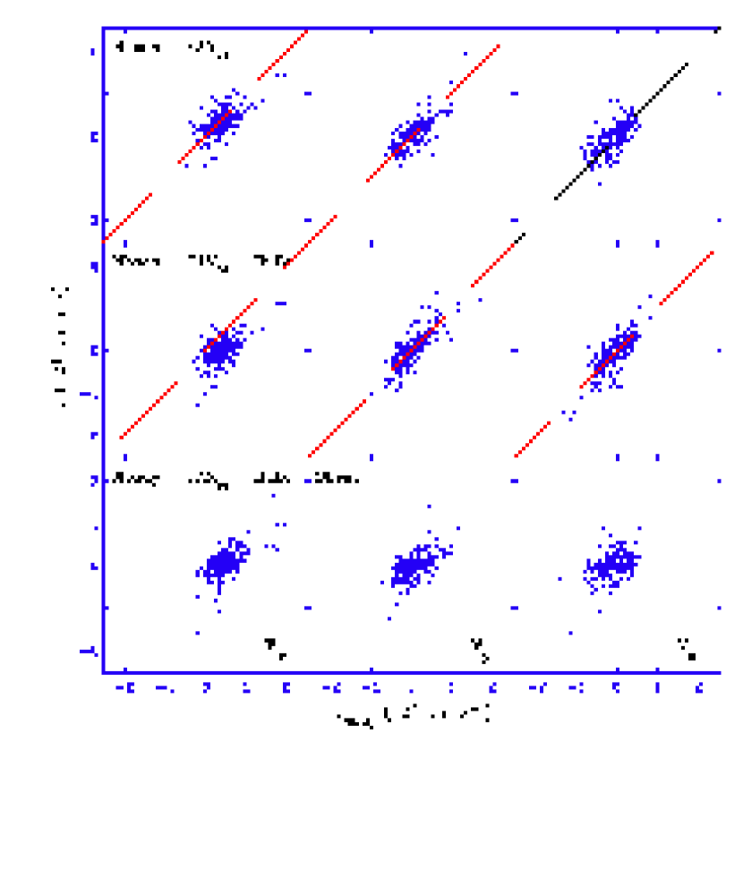
Figure 15: point-to-point comparison between the three successive residual velocities and the corresponding mock catalog $N$-body velocity. The three panels in each row correspond to the $x$, $y$ and $z$ velocity components. The coordinate system is the “shear reference system”. Top row: the tidal velocity field $N$-body-$FAM$. Middle row: residual velocity field after subtraction bulk flow. Bottom row: residual velocity field after subtraction of both tidal bulk and shear components.

The “shear ellipsoid”, the quadratic surface defined by the shear tensor ${\tilde{s}^{\prime}}_{ij}$ with principal axes aligned along the eigenvectors and with axis size set by the corresponding eigenvalue $s_{i}$, defines a natural reference system to assess the tidal shear flow field. The coordinate axes of this “shear reference frame” are identified with the orthonormal basis defined by the (normalized) eigenvectors. The $x$-axis is chosen to be aligned along the major axis of the “shear ellipsoid”, the direction defined by the largest (positive) eigenvalue $s_{1}$ and directed along the strongest dilational (stretching) motion incited by the external tidal field. Likewise the $z$-axis is chosen to coincide with the lowest (negative) eigenvalue $s_{3}$, aligned along the strongest “compressional” component of the tidal velocity flow. This leaves the $y$-axis as the one coinciding with the intermediate eigenvalue $s_{2}$.

The imprint of the shearing motions can be discerned within the $y-z$ plane and, most prominently, along the “x-z” projection of the “bulk flow reference system”. After subtraction of the bulk flow component, i.e. $N$-body-FAM₃₀-$v_{bulk}$, the quadrupolar component of the externally induced velocity flow represents its principal constituent (Fig. 13, lower row). This is confirmed by the values quoted in Table 4 for the shear contribution. In particular when stated in the velocity equivalent unit of $\ {\rm km\leavevmode\nobreak\ s^{-1}}$ these shear values suggest that the quadrupolar shear contributions are of a comparable magnitude to those of the bulk flow. The maps in the lower row of Figure 13 suggest that there are strong dilational and compressional motions within the $y-z$ plane. By contrast, the shear motions in the $x$-direction appear to be uncommonly weak. Given the “bulk flow reference system”, it implies that for this particular realization we see a bulk flow directed almost perpendicular to the shear flow motions.

Cosmology	$R_{Spear}$	$R_{lin}$	$a_{0}$	$a_{lrg}$	$\sigma_{lrg}$
			(km s-1)		(km s-1)
$\Lambda$CDM	0.62  $\pm$  0.17	0.58  $\pm$  0.22	-4.03  $\pm$  75.45	0.83  $\pm$  0.20	246  $\pm$  134
$\tau$CDM	0.75  $\pm$  0.11	0.71  $\pm$  0.14	-9.31  $\pm$  30.19	0.93  $\pm$  0.13	219  $\pm$   86

Table 5: Average final results for the $N-$body velocities $vs.$ the corrected FAM₃₀ after adding to it the tidal Bulk and Shear contributions. The errors represent the $1\sigma$ scatter around the average value. Col. 1: Cosmological model. Col. 2: non parametric (Spearman) correlation coefficient. Col. 3: linear correlation index. Col. 4: zero point of the best linear fit. Col. 5: slope of the best fitting line. Col. 6: dispersion around the fit.

Figure 14 depicts the same $\Lambda$CDM mock sample as presented in Figs. 7, 8 & 13, here in the “shear reference frame”. The top row shows the full externally induced flow field, $N$-body - FAM₃₀, in this reference system. The tidal shear flows are almost exclusively confined to the $x-z$ plane. This is most evidently illustrated in the central row of frames showing the velocity field without its bulk flow component: hardly any systematic flow is noticeable in the $y$-direction of the intermediate shear eigenvalue.

8.4 Multipole Scale Dependence

When turning to the external influences over a large $100h^{-1}{\rm Mpc}$ region, we may conclude from the second section of the table that most of the external contributions are accounted for, both bulk flow and shear are at least a factor of 3-4 smaller than for the inner $30h^{-1}{\rm Mpc}$ region. The third and fourth section show that the explicit contributions from the regions between $100h^{-1}{\rm Mpc}$ and $30h^{-1}{\rm Mpc}$ and those beyond $100h^{-1}{\rm Mpc}$ are indeed significantly different, those beyond $100h^{-1}{\rm Mpc}$ tending towards zero contributions and as far as the shear is concerned almost an order of magnitude smaller than the equivalent contributions by the $30-100h^{-1}{\rm Mpc}$ region.

A similar graphical assessment involving the FAM₁₀₀ reconstructions emphasizes the minor significance of tidal contributions stemming from density fluctuations beyond a radius of $100h^{-1}{\rm Mpc}$. No coherent velocity pattern can be recognized in the residual velocity field between full $N$-body and FAM₁₀₀ reconstruction. The comparison between this residual velocity field with the velocity maps including the contributions of the inferred bulk flow and shear flow do hardly show any difference. In all cases the velocity fields are dominated by the same thermal motions.

8.5 Multipole Velocity Flow Model

Following our argument that the externally induced velocity flow within the inner $30h^{-1}{\rm Mpc}$ mainly consists of a bulk flow and shear contribution, we may expect that the effect of the external gravity field can be sufficiently accounted for by adding these components to a local velocity field model based on the mass distribution in and around the Local Superclusters.

By separating the “internal” FAM velocity field from the “external” multipole contributions of the (monopole,) dipole and quadrupole components of the “tidal” velocity field and adding the two, we obtain a total “FAM-multipole” model velocity ${v_{fam-mpl,i}}$,

$$v_{fam-mpl,i}\,\approx\,v_{FAM,i}\,+\,v_{exp,i}+v_{bulk,i}\,+\,v_{shear,i}$$ (31)

A visual impression of the extent of the successive multipole contributions may be obtained from Fig. 12. The vector plots of the four velocity contributions to $v_{fam-mpl}$ (Eq. 31) are depicted in four successive rows, each within the mutually perpendicular three central slices (wrt. the shear reference system). The top row concerns the FAM₃₀ velocity field reconstruction, followed successively by the expansion/contraction term (monopole), the bulk flow (dipole) and velocity shear (quadrupolar).

From fig. 13 and fig. 14 we conclude that the differences between the “full” $N$-body velocities and $v_{fam-mpl}$, the total sum of the internal FAM₃₀ and external dipole and quadrupole contributions, do not appear to show systematic trends as it can be noticed from the residual bulk and shear components in section 4 of Table 4. Wherever there are large deviations, these are mainly confined to the high density virialized regions.

8.6 Point-to-Point Comparison

A quantitative quality assessment of the “FAM-multipole” model is offered by the point-to-point comparison between the full $N$-body velocity and its difference with respect to the successive modes of the “FAM-multipole” velocity in Fig. 15. The $v_{x}$, $v_{y}$ and $v_{z}$ of the various velocity components refer to the “bulk flow reference system”. The top row, plotting $v_{Nbody}$ vs. the residual $N$-body-FAM₃₀, reveals the expected systematic differences due to missing externally induced contributions. Given the fact that the bulk flow in this reference system is confined to the $x$-component, we may note the uniform systematic shift of the $x$ residuals with respect to the zeropoint $(v_{Nbody},v_{res})=(0,0)$ (top lefthand frame). The subsequent addition of the dipolar bulk flow contribution to FAM₃₀ leads to a systematic downward uniform vertical shift of $N$-body-FAM₃₀-Bulk (middle row Fig. 15): also the residuals in the $x$-direction now center on $v_{res}=0$ (note that by virtue of the bulk flow the $N$-body velocities in the $x$-direction are also skewed to values larger than $v_{Nbody}=0$).

The three point-to-point diagrams in the middle row of Fig. 15 show that even while the bulk flow is taken into account systematic motions remain in all three directions. The point-to-point comparisons still follow a strong correlation with respect to the the $N$-body  velocities. It mainly involves the presence of the quadrupolar velocity shear component (in addition to a minor ingredient contributed by the monopole expansion/contraction term). This can be immediately inferred from the comparison between the diagrams in the central and lower row of Fig. 15: once the quadrupole component “Shear” has been added to the “FAM₃₀+Bulk” velocities the systematic effects seem to have largely vanished. What remains in the residuals is mainly random scatter, centered on the $v_{res}=0\ {\rm km\leavevmode\nobreak\ s^{-1}}$ line, with some exceptional outliers originating in the virialized regions.

We have quantified the point-to-point comparisons by performing linear regressions similar to those presented in Section 7. Table 5 summarizes the results of this comparison for all catalog samples for both cosmologies. In both cosmological models the slope of the best fitting line is consistent with unity at $\sim 1\sigma$ confidence level. As expected, the scatter around the fit is similar to that of all previous analyses (see Table 3). Offsets around the zero-point are consistent with zero, although with a large dispersion. The strength of the point-to-point correlations has increased considerably with respect to their FAM₃₀ counterpart (Table 3) and it is very similar to the FAM₁₀₀ case.

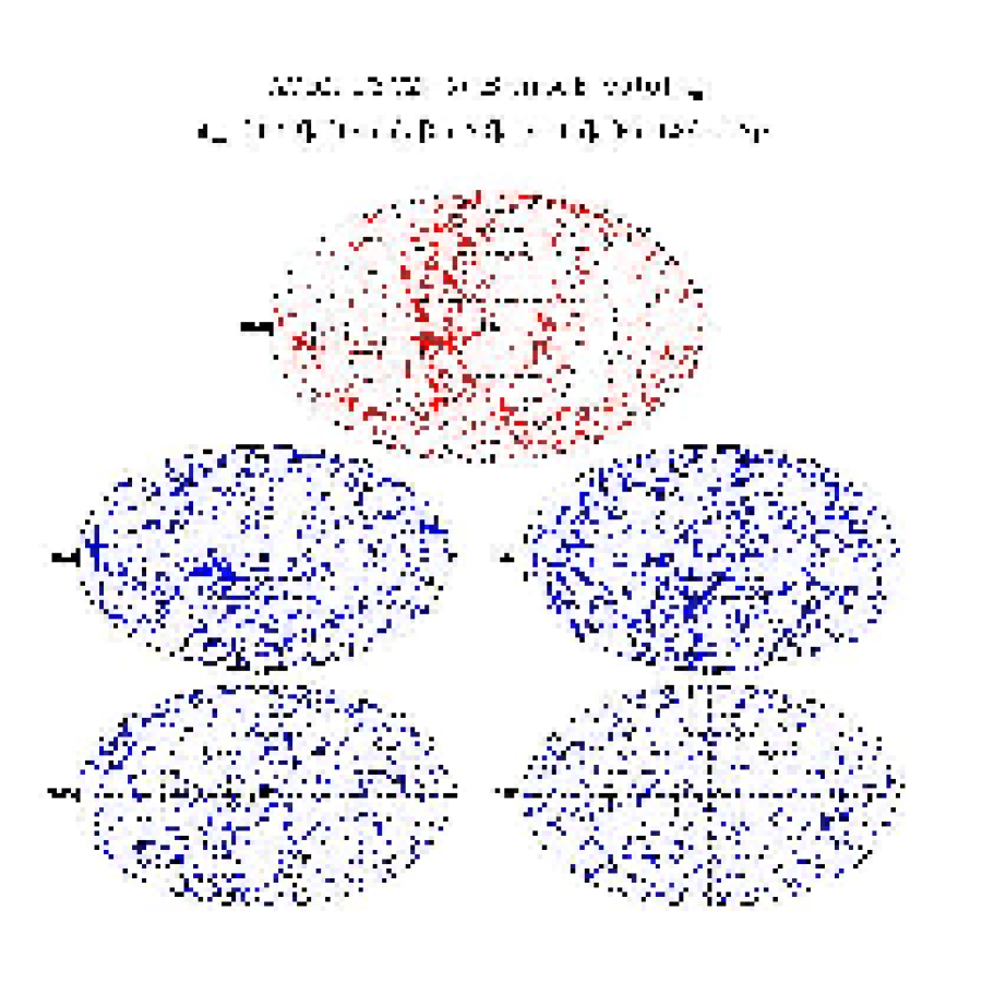
Figure 16: Aitoff projections of the galaxy distribution of a NBG + PSC$z$  $\Lambda$CDM catalog. The top-most panel shows the corresponding NBG distribution, $d_{sur}=[0,30]h^{-1}{\rm Mpc}$. The subsequent panels depict the external galaxy distribution enclosed by the shells defined by survey depth $d_{sur}=[30-55]h^{-1}{\rm Mpc}$, $d_{sur}=[55-70]h^{-1}{\rm Mpc}$ $d_{sur}=[70-85]h^{-1}{\rm Mpc}$ and $d_{sur}=[85-100]h^{-1}{\rm Mpc}$.

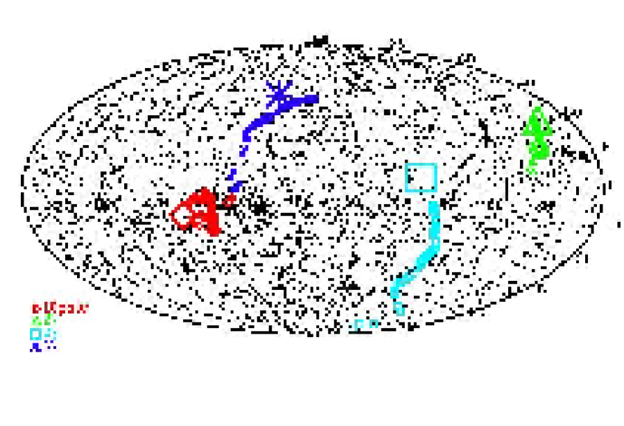
Figure 17: Sky distribution of galaxies in external shell of survey depth $d_{sur}=30-100h^{-1}{\rm Mpc}$. This galaxy distribution should reflect the mass distribution inducing the local tidal velocity flow. By means of symbols we have indicated the track of the gravity dipole and quadrupole eigenvector directions (cf. eqn. 35 and eqn. 36) on the sky, by radially expanding outward the survey depth $d_{sur}$ in steps of $1h^{-1}{\rm Mpc}$, from $d_{sur}=30h^{-1}{\rm Mpc}$ to $d_{sur}=100h^{-1}{\rm Mpc}$. For comparison the same symbol, but then enlarged, indicates the directions for the corresponding bulk velocity and velocity shear eigenvector directions. Diamond: dipole. Triangle: stretching component shear. Square: middle component shear. Star: compressional component shear.

8.7 Surrounding Matter Distribution: Tidal Source

The surrounding external matter distribution is the source for the tidal velocity field which we inferred in the previous sections. For various purposes we wish to relate the computed dipolar bulk flow and quadrupolar shear flow components to the surrounding matter distribution which induced them.

The induced tidal velocities involve spatial scales ranging from $30h^{-1}{\rm Mpc}$ to $100h^{-1}{\rm Mpc}$. Over this range the linear theory of gravitational instability holds to good approximation. This translates into a direct linear relationship between induced velocity ${\bf v}_{ext}$ and the cumulative external gravitational force ${\bf g}_{ext}$,

$${\bf v}_{ext}({\bf x},t)\,=\,{\displaystyle 2f(\Omega,\Lambda)\over\displaystyle 3H\Omega}\,{\bf g}_{ext}({\bf x},t)\,,$$ (32)

with $f(\Omega,\Lambda)$ the linear velocity growth factor. This linear relationship also holds for every component of the velocity and gravity fields, and thus also for the individual dipolar and quadrupolar components of the externally induced velocity field. They are directly proportional to equivalent dipole and quadrupolar components of the gravity field:

$${\bf v}_{bulk}({\bf x},t) \,=\, \,\,\,\,{\displaystyle 2f(\Omega,\Lambda)\over\displaystyle 3H\Omega}\,\,{\bf g}_{bulk}({\bf x},t)$$

$$s_{ij}({\bf x},t) \,=\, -{\displaystyle 2f(\Omega,\Lambda)\over\displaystyle 3H\Omega}\,\,{\cal T}_{ij}({\bf x},t)$$ (33)

with the (external) gravitational tidal shear tensor ${\cal T}_{ij}$ is defined as (see van de Weygaert & Bertschinger rienbert (1996)),

$${\cal T}_{ij}\,=\,{\displaystyle\partial^{2}\Phi_{tidal}\over\displaystyle\partial x_{i}\partial x_{j}}\,.$$ (34)

Notice that because of its external nature, the term ${\displaystyle 1\over\displaystyle 3}\nabla^{2}\Phi_{tidal}\,\delta_{ij}$ is always equal to zero.

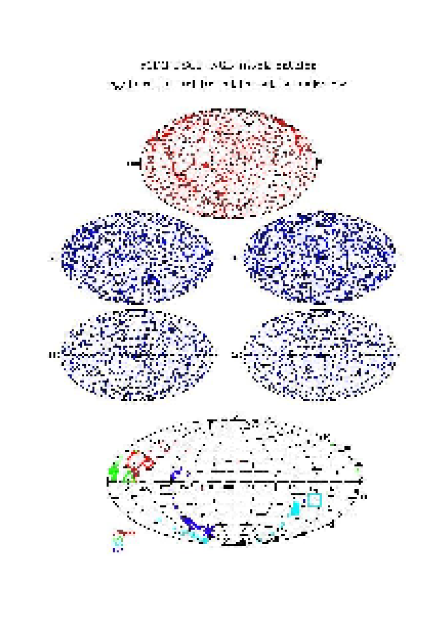
Figure 18: Aitoff projections of the galaxy distribution of a NBG + PSC$z$  $\tau$CDM catalog. The top-most panel shows the corresponding NBG distribution, $d_{sur}=[0,30]h^{-1}{\rm Mpc}$. The subsequent 4 panels depict the external galaxy distribution enclosed by the shells defined by survey depth $d_{sur}=[30-55]h^{-1}{\rm Mpc}$, $d_{sur}=[55-70]h^{-1}{\rm Mpc}$ $d_{sur}=[70-85]h^{-1}{\rm Mpc}$ and $d_{sur}=[85-100]h^{-1}{\rm Mpc}$. Bottom panel: convergence gravity dipole and quadrupole. By means of symbols we have indicated the track of the gravity dipole and quadrupole eigenvector directions (cf. eqn. 35 and eqn. 36) on the sky, by radially expanding outward the survey depth $d_{sur}$ in steps of $1h^{-1}{\rm Mpc}$, from $d_{sur}=30h^{-1}{\rm Mpc}$ to $d_{sur}=100h^{-1}{\rm Mpc}$. For comparison the same symbol, but then enlarged, indicates the directions for the corresponding bulk velocity and velocity shear eigenvector directions. Diamond: dipole. Triangle: stretching component shear. Square: middle component shear. Star: compressional component shear.

Ideally, we would like to infer the external tidal potential $\Phi_{tidal}$ directly from the galaxy distribution in a sufficiently large surrounding region. This is specifically true for its dipolar and quadrupolar moments, with the intention to insert these terms directly into the expression for the FAM potential (eqn. 12 and eqn. 10). The required externally induced bulk flow velocity and velocity shear should be the result. The comparison of the FAM computed velocities for the local volume, in combination with the computed tidal velocities (Sec. 8.2), and the observed and measured velocities would then enable us to determine the amount of mass and average density in the local volume.

To determine the gravitational influence of the surrounding matter distribution, we set out to assess the sky distribution of galaxies in the local NBG volume, out to $r_{NBG}=30h^{-1}{\rm Mpc}$, along with the external mass distribution in radial shells out to a distance $r_{PSCz}\leq 100h^{-1}{\rm Mpc}$. A prominent dipolar matter configuration in the sky distribution will translate into a strong bulk gravity force. Similarly, quadrupolar anisotropies will translate into an effective tidal shear force. In figure 16 we have plotted the galaxies in one of our $\Lambda$CDM mock catalogs in five successive distance shells. Aitoff projections of the angular positions of the galaxies, as seen from the centre of the local NBG volume, provide an impression of the level of anisotropy in the mass distribution at successive radii.

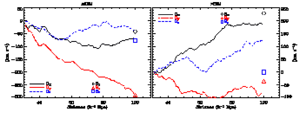
Figure 19: Cumulative gravity dipole and tidal gravity shear. As a function of survey depth $d_{sur}$ the Cartesian components of the gravity dipole, $g_{x}$, $g_{y}$ and $g_{z}$ is followed (in equivalent velocity unit $\ {\rm km\leavevmode\nobreak\ s^{-1}}$). The symbols at $d_{sur}$ indicate the corresponding velocity dipole. Lefthand panel: $\Lambda$CDM. Righthand panel: $\tau$CDM.

The first sky plot (top sphere) depicts the sky position of the galaxies in the local NBG-mimicking mock sample. It involves a highly flattened distribution, perhaps reminiscent of the Supergalactic Plane. The four subsequent shells correspond to successive cuts through the PSCz mimicking samples, at sampling depths $d_{sur}=[0-30],\,[30-55],\,[55-70]$ and $[85-100]\,h^{-1}{\rm Mpc}$. The first and direct observation is the diminishing sample density as a function of survey depth, in accordance with the selection function (eqn. 19). Structure is most prominent in the first shell, at $d_{sur}=[30-55]\,h^{-1}{\rm Mpc}$ (central left sphere). The structure contained in this shell also shows a clear affiliation with the matter distribution in the local NBG volume. The compact massive concentration at $l\approx 220^{\circ}$ is clearly connected to a dense region in the local “plane”. A superficial inspection of the angular galaxy distribution reveals the presence of strong dipolar and quadrupolar components, effecting considerable tidal forces. Note that both external shells display a rather strong concentration of galaxies in their southern hemisphere, in the vicinity of $l\approx 180-200^{\circ}$. Similar but weaker contributions can also be recognized from the galaxy distribution in the shell between $d_{sur}\approx 70-85h^{-1}{\rm Mpc}$. Beyond $d_{sur}>85h^{-1}{\rm Mpc}$, however, the angular pattern appear to be considerably less pronounced. This is in line with the earlier findings that there were hardly noticeable tidal contributions from large distances.

To see to what extent the depicted galaxy distribution can indeed be held responsible for most of the inferred tidal bulk flow and tidal shear, we have determined the corresponding bulk force ${\bf g}_{bulk}$ (eqn. 4) and tidal shear ${\cal T}_{ij}$ (eqn. 5) evoked by the external galaxy distribution ($r>30h^{-1}{\rm Mpc}$). Since we do not have a continuous density field but the positions of a finite number of objects in our galaxy flux-limited and full mass distribution catalogs, the bulk acceleration on the LG is computed from the discrete equivalent. For a sample of galaxies at locations ${\bf x}_{i}$, with an average number density $n$ of selected objects, this leads to

$${\bf g}_{bulk}\,=\,{\displaystyle H\,f(\Omega,\Lambda)\over\displaystyle 4\pi n}\,\sum_{i}\,{1\over\displaystyle\psi(x_{k})}\,{\displaystyle{\bf x}_{k}\over\displaystyle|{\bf x}_{k}|^{3}}\,.$$ (35)

where $\psi(x_{k})$ is the sample selection function at distance $x_{k}$, whose inverse functions as weighting factor. For practical reasons, comparison with the inferred bulk flow ${\bf v}_{bulk}$, we have translated the bulk acceleration into equivalent velocity units by means of the transformation $Hf(\Omega,\Lambda)/{3\over 2}\Omega H^{2}$. The equivalent “discrete” expression for the external tidal shear is

$${\cal T}_{ij}\,=\,{\displaystyle H\,f(\Omega,\Lambda)\over\displaystyle 4\pi n}\,\sum_{i}\,{\displaystyle 1\over\displaystyle\psi(x_{k})}{\displaystyle 3\,x_{ki}\,x_{kj}\over\displaystyle|{\bf x}_{k}|^{5}}\,.$$ (36)

For the $\Lambda$CDM mock galaxy sample depicted in Fig 16 we determine the gravity dipole by computing for a set of spherical external shells the resulting bulk flow acceleration (eq. 35) and the gravity quadrupole by computing external tidal shear (eq. 36). Recently, a similar approach was followed by Teodoro et al. teod2004 (2004). The spherical shell volumes are defined by an inner radius $r_{inn}=30h^{-1}{\rm Mpc}$ and an outer radius $r_{out}$. The width of the shell is gradually enlarged by increasing $r_{out}$ from $r_{out}=30h^{-1}{\rm Mpc}$ to $r_{out}=100h^{-1}{\rm Mpc}$. The convergence of the resulting gravity dipole direction on the sky can be observed in Fig. 17. The small red diamonds are consistently located near $l\approx 230^{\circ}$, and converge at a sky location close to the direction of the velocity dipole (large red diamond). To get an idea of the amplitudes involved, Fig. 19 (top panel) shows the development of the cumulative gravity dipole as a function of external distance $d_{sur}$ ($30h^{-1}{\rm Mpc}<d_{sur}<100h^{-1}{\rm Mpc}$). By means of symbols the corresponding velocity dipole, for each of the three directions $x$, $y$ and $z$, are inserted at the outer radius of $d_{sur}\approx 100h^{-1}{\rm Mpc}$. Note that we have restricted ourselves to a case study example. A more extensive and proper assessment, including a proper error estimate of both gravity dipole and quadrupole as well as the bulk and shear flow, is beyond the scope of the present argument. This issue, involving the shot noise influence on gravity dipole and quadrupole and the role of FAM uncertainties on the velocity flow components, will be treated in more detail in a forthcoming study.

We see that in the $x$-, $y$ and $z$-directions of the gravity and velocity dipoles are in reasonable agreement, within a margin of $\approx 30\ {\rm km\leavevmode\nobreak\ s^{-1}}$. This observation justifies our expectation that the dipole can be estimated to sufficient accuracy from the surrounding external galaxy distribution. The dipole may then be estimated from the surrounding external galaxy distribution, so that the latter can be invoked to correct for the influence of the external tidal field in the dynamics of the local volume.

The situation is comparable for the cumulative tidal shear, in terms of its three eigenvalues and eigenvectors. Also the gravity quadrupole appears to converge relatively smoothly towards the velocity shear. This may be inferred from the plotted directions of the eigenvectors ${\hat{\bf e}}_{{\cal T}1}$, ${\hat{\bf e}}_{{\cal T}2}$ and ${\hat{\bf e}}_{{\cal T}3}$ of the tidal shear ${\cal T}_{ij}$. They are indicated by means of three symbols, the triangle corresponding to the stretching component ${\cal T}_{1}$, the star the middle component ${\cal T}_{2}$ and the square the compressional component ${\cal T}_{3}$. The tidal shear tensor wanders extensively across the “sky” as we push the outer radius of the external shell outward, as is shown by the paths of the corresponding eigenvectors. Interestingly, once the shell radius starts to approach $100h^{-1}{\rm Mpc}$, each of the eigenvectors appear to converge near the location of the corresponding stretching, central and compressing velocity shear tensor eigenvectors. However, also here we notice significant deviations in individual cases.

For comparison, we can appreciate the role of the external tidal field on local dynamics for the case of the $\tau$CDM cosmology. Figure 18 combines the galaxy sky distribution for a $\tau$CDM mock galaxy sample, in the same radial shells as in Fig. 16. The final frame shows the Aitoff projection of the gravity dipole and gravity quadrupole eigenvectors for a set of gradually increasing radial shells. From the galaxy sky distribution in the four slices at sampling depths $d_{sur}=[0-30],\,[30-55],\,[55-70]$ and $[85-100]\,h^{-1}{\rm Mpc}$ we notice that these involve considerably more isotropic distributions. Hardly any prominent patterns can be discerned in the sky distribution. This is expressed in a more erratic wandering of gravity dipole and quadrupole directions (lower frame, fig. 16). This also implies a more substantial contribution of shot noise effects. The latter represent a major source for deviations between the velocity dipole and shear flow quadrupole and the gravity dipole and quadrupole. The smaller coherence length of the $\tau$CDM fluctuations and the more randomly oriented contributions by the individual external matter concentrations may therefore be directly related to the lower level of coincidence between velocity and gravity directions than in the case of the more prominent anisotropies in the $\Lambda$CDM cosmology. In this, we have to realize that the amplitude of dipole and quadrupolar contributions between the two scenarios are not too different (cf. table 5). The less prominent anisotropies in the $\tau$CDM catalogues are therefore compensated by a higher average matter density.

8.8 Multipole Components: Summary

The above results reassure the fact that the external tidal field can be well characterized by its main multipole components, the bulk flow and velocity shear. In terms of multipole amplitude convergence, these results show a better agreement for the $\Lambda$CDM model than for the $\tau$CDM one. This is due to the intrinsic characteristics of both cosmic models. As has been discussed in Section 4, and may be directly appreciated from Fig. 2, the relatively lower amplitude of the $\tau$CDM perturbations is compensated by a higher mass content. It leads to an equally strong external gravitational influence. On the other hand, the smaller spatial coherence of density features in the $\tau$CDM scenario causes the orientation of the gravity dipole and quadrupoles to be rather jittery. The direction of the cumulative gravitational force in the $\tau$CDM scenario wanders erratically over the sky as we move further out from the local volume. This differs from the situation in the $\Lambda$CDM samples, where we observe a consistent, systematic and coherent convergence towards the final dipole direction.

The above results confirm the fact that the external tidal velocity field can be well characterized by its main multipole components, the bulk flow and velocity shear. This depends to some extent on the cosmology. In terms of multipole amplitude convergence, these results show a better agreement for the $\Lambda$CDM than for the $\tau$CDM model.

9 Conclusions

In this work we have applied the FAM technique to construct model velocity fields using mock catalogs resembling the NBG and IRAS-PSC$z$ galaxy catalogs. The mock catalogs were extracted from $N$-body simulations in which the central observer mimics some of the properties of the Local Group environment. Comparing FAM velocities obtained from the NBG mock catalogs with those obtained from the larger PSC$z$ mock catalogs and, finally, to the $N$-body velocities, allowed us to quantify the importance of the gravity field generated by the mass distribution within and beyond the LS.

Neglecting the mass distribution outside the LS leads to a systematic underestimate of the gravity field. The amplitude of this bias depends on the amount of power on scales larger than the LS, and thus on the cosmological models. In a $\tau$CDM universe model peculiar velocities are $\sim 20\%$ smaller than the true ones. In the case of a $\Lambda$CDM model, which has more power on large scales, model velocities are underestimated by $\sim 35\%$.

The results of the described FAM analyses are encouraging in the sense that the presently available all-sky, flux limited catalogs such as PSC$z$ appear to be capable of accounting for the major share of the velocity field on the scale of the Local Supercluster. While the $30h^{-1}{\rm Mpc}$ restricted NBG sample showed a substantial deficiency in its capacity to generate the local cosmic motions, in particular in the case of the $\Lambda$CDM Universe models, in both cases the $100h^{-1}{\rm Mpc}$ mock samples appear to embody nearly all matter concentrations responsible for the generated velocities in our local (NBG catalog) neighbourhood.

Also we notice a telling difference between the performance of both FAM₃₀ and FAM₁₀₀ reconstructions for the case of the $\Lambda$CDM cosmology catalogs on the one hand and the $\tau$CDM model catalogs on the other hand. The fact that the $\Lambda$CDM model involves substantially more power on large scales, $r>30h^{-1}{\rm Mpc}$, than the $\tau$CDM model is reflected in the better quality of the FAM₃₀ reconstructions for the $\tau$CDM catalogs. The presence of substantial mass inhomogeneities with a scale in excess of that of the local Universe regions implies a larger external contribution to the local velocity field. This is also borne out by the fact that for the $\Lambda$CDM catalogs we see a considerable improvement in velocity field reconstruction quality going from the FAM₃₀ to the FAM₁₀₀ reconstructions (see Table 4), while this is far less so for the $\tau$CDM catalogs.

Of course, whether the resulting models do indeed form an unbiased representation of the actual velocity field will to some extent also depend on whether the galaxy distribution in the flux limited galaxy catalogs does represent an unbiased reflection of the actual (external) mass distribution surrounding the Local Supercluster resembling region. The results of recent studies (Verde et al. verde2002 (2002), Lahav et al. lahav2002 (2002), Tegmark, Zaldarriaga & Hamilton tegzalham2001 (2001) and Branchini, Dekel & Sigad brandeksig2002 (2002)) are quite encouraging in this respect. They seem to indicate, certainly on scales larger than $\approx 5h^{-1}{\rm Mpc}$, that both IRAS and 2dF galaxies trace the underlying mass distribution in an unbiased fashion.

Nonetheless, observations along the lines of the presented mock catalogs seem to suggest that a proper analysis of Local Universe dynamics based on a combination of information of local small-scale (peculiar) galaxy velocities and a rough yet well-founded idea of the matter distribution on scales of a few hundred $100h^{-1}{\rm Mpc}$ may help us towards acquiring far more insight into the dynamical history of the emergence and assembly of the striking nonlinear patterns we have discovered in the large scale matter distribution. Moreover, we have uncovered evidence that a meticulous point-to-point analysis of such velocity samples may help towards modelling the total local force field, including a proper model for the external forces.

When modeling the peculiar velocity of a LS look-alike region by only considering the matter distribution within $30h^{-1}{\rm Mpc}$, the end product is a biased velocity field lacking of any large scale signature. This bias can be eliminated by accounting for the mass distribution beyond the LS. Our experiments demonstrate that sampling the mass distribution out to scales of $100h^{-1}{\rm Mpc}$, in a flux limited fashion, is sufficient to account for the large scale contribution to the peculiar velocities in our cosmological neighborhood. More precisely, we have found that the cosmic velocity field within the LS, modeled by FAM using the mass distribution traced by PSC$z$ galaxies out to $100h^{-1}{\rm Mpc}$ is unbiased. The differences between true and FAM velocity field are random and mainly occur in high density environments which are dominated by virial motions that are not modeled correctly by FAM.

The gravity and velocity fields generated by the mass distribution beyond the scale of the Local Supercluster are well characterized by their bulk flow and shear components. Therefore, one can obtain an unbiased model velocity field by superimposing a local model velocity field within the Local Supercluster to the bulk flow and shear components of the velocity field generated by the mass distribution between 30 and $100h^{-1}{\rm Mpc}$.

These considerations suggest that velocity models which only consider the dynamics within the Local Superclusters might have been affected by systematic errors. In particular, our work suggests that, when compared with observed velocities, they might have underestimated the value of the density parameter, $\Omega_{m}$, by 15-25 %. However, the analysis of Shaya, Tully and Peebles (shaya (1995)), based on the galaxy distribution in the Local Supercluster, shows that a lower, not a larger, value of $\Omega_{m}$ is found when complementing the local mass distribution with the large scale one traced by rich Abell clusters. A more precise evaluation of this bias will be performed in a future work in which we will perform the same analysis presented here using a new set of mock catalogs that are constrain to reproduce the distribution of the mass in our local Universe (see e.g. van de Weygaert & Hoffman vdwhof (1999), Mathis et al. mathis2002 (2002), Klypin et al. klypin (2003)).

Furthermore, our analysis shows that all model velocity fields of the Local Supercluster which are based on the PSC$z$ catalog (e.g. Branchini et al. branchini99 (1999), Schmoldt et al. schmoldt99 (1999), Valentine et al. valentine (2000), Sharpe et al. sharpe (2001)) are free from systematic biases arising from having neglected the large scale contribution from scales beyond its realm. Moreover, since the IRAS PSC$z$ survey is considerably deeper than $100h^{-1}{\rm Mpc}$, it is reasonable to assume that the PSC$z$ catalog can be used to predict unbiased velocities well beyond our Local Supercluster that, if compared with observed galaxy peculiar velocities, can discriminate among different cosmologies characterized by different values of $\Omega_{m}$, like the $\Lambda$CDM and $\tau$CDM models.

The plausibility of this hypothesis has been recently confirmed by the analysis of Hoffman et al. (hoffman01 (2001)) that shows that the bulk and shear components of the external velocity field in the local universe inferred from the peculiar velocities in the Mark III catalog (Willick et al. 1997a , 1997b ) are qualitatively consistent with those expected from the mass distribution traced by IRAS PSC$z$ galaxies. On the other hand, the claim on the basis of the SMAC cluster peculiar velocity sample (Hudson et al. hudsv (2004)) of an extra $225\ {\rm km\leavevmode\nobreak\ s^{-1}}$ bulk flow component generated by matter concentrations on a scale exceeding $100h^{-1}{\rm Mpc}$ should issue some caution with respect to claims of having accounted for all external influences on the local cosmic flow.

Coupling the local velocity model provided by FAM to the large scale contribution provided by linear theory allows to obtain a model velocity field which is unbiased, nonlinear and fast to compute. This means that, for the first time, we are in the position of performing a large number of experiments aimed at studying the nonlinear evolution of cosmic structures, such as filaments and clusters, and explore the role of tidal fields during their gravitational collapse. This relates to the observation that filaments are forming as a consequence of anisotropic collapse, induced a compressional tidal force acting perpendicular to the “axis” of the filament. By tracing out the coherent paths of the compressional modes of the primordial tidal field one can identify the sites of the later nonlinear filaments (Bond et al. cosmweb (1996), see Van de Weygaert weyfoam (2002)). In turn this is directly related to cluster locations: the strong primordial tidal shear is the result of a local quadrupolar mass distribution. The corresponding overdensities tend to evolve into rich clusters, explaining the intimate link of clusters and filaments in the cosmic web.

Finally, it is worth stressing that in this work we have neglected the fact that we measure galaxy redshifts rather then positions. By means of an elegant formalism, Phelps phelps2000 (2000) demonstrated the feasibility of working out the action principle in redshift space. With respect to FAM, Nusser & Branchini (nusbran (2000)) have shown that it can be easily implemented in redshift space and Branchini, Eldar & Nusser (branchini02 (2002)) demonstrated that it performs equally well in real and redshift space. Therefore, our unbiased, nonlinear model velocity field also allows to perform an accurate correction for redshift space distortions and thus lead to a precise reconstruction of the mass distribution in real space. Mapping the mass in the local universe down to nonlinear scales and comparing it with the distribution of baryonic mass (in form of stars or diffuse, ionized gas) is of considerable astrophysical interests as it will constrain and help understanding the process of galaxy formation and evolution within the Universe

- (1) Bardeen J.M., Bond J.R., Kaiser N., Szalay A.S., 1986, ApJ, 304,15
- (2) Berlind A.A., Narayanan V.K., Weinberg, D. H., 2000, ApJ, 537, 537
- (3) Bond J.R., Efstathiou G., 1991, Phys. Lett. B., 265, 245
- (4) Bond J.R., Kofman L., Pogosyan D. Yu., 1996, Nature, 380, 603
- (5) Bouchet F., Hernquist L., 1988, ApJS, 68, 521
- (6) Branchini E., Carlberg R., 1994, ApJ, 434, 73
- (7) Branchini E., Teodoro L., Frenk C. S., Schmoldt I., Efstathiou G., White S. D. M., Saunders W., Sutherland W., Rowan-Robinson M., Keeble O., Tadros H., Maddox S., Oliver S., 1999, MNRAS, 308, 1
- (8) Branchini E., Eldar A., Nusser A., 2002, MNRAS, 335, 53
- (9) Branchini E., Freudling W., Da Costa L. N., Frenk C. S., Giovanelli R., Haynes M. P., Salzer J. J., Wegner G., Zehavi I., 2001, MNRAS, 326, 1191
- (10) Branchini E., Dekel A., Sigad Y., 2002, MNRAS, submitted
- (11) Carlberg R., Couchman H., Thomas P., 1990, ApJ, 352, L29
- (12) Cole S., 1997, MNRAS, 286, 38
- (13) Cole S., Hatton S., Weinberg D.H., Frenk C.S., 1998, MNRAS, 300, 945
- (14) Colless M., the 2dFGRS team, 2003, astro-ph/0306581
- (15) Colless M., 2004, in Measuring and Modeling the Universe, ed. W.L. Freeman, Carnegie Obs. Astrophys. Ser., vol. 2, in press (astro-ph/0305051)
- (16) da Costa L.N., Bernardi M., Alonso M.V., Wegner G., Willmer C.N.A., Pellegrini P.S., Rit C., Maia, M. A. G., 2000, AJ, 120, 95
- (17) Croft R.A.C., Gaztañaga E., 1997, MNRAS, 285, 793
- (18) Davis M., Nusser A., Willick J.A., 1996, ApJ, 473, 22
- (19) Dekel, A., 1994, ARAA, 32, 371
- (20) De Lapparent V., Geller M.J., Huchra J.P., 1986, ApJ, 302, L1
- (21) Dunn A.M., Laflamme R., 1993, MNRAS, 264, 865
- (22) Eke V., Cole S., Frenk C., 1996, MNRAS, 282, 263
- (23) Faber & Burstein, 1988, in The Vatican Study Week on Large Scale Motions in the Universe, ed. G. V. Coyne & V. C. Rubin (Princeton: Princeton Univ. Press), 115
- (24) Fisher K.B., Huchra J.P., Strauss M.A., Davis M., Yahil A., Schlegel D., 1995, ApJS, 100, 69
- (25) Han M., Mould J., 1990, ApJ, 360, 448
- (26) Giavalisco M., Mancinelli P.J., Mancinelli P.J., Yahil A., 1993, ApJ, 411, 9
- (27) Giovanelli R., Haynes M.P., Herter T., Vogt N.P., Wegner G., Salzer J.J., da Costa L.N., Freudling, W., 1997, AJ, 113, 22
- (28) Giovanelli R., Haynes M. P., Herter T., Vogt N. P., da Costa L.N., Freudling W., Salzer J.J., Wegner G., 1997, AJ, 113, 53
- (29) Goldberg D.M., Spergel D.N., 2000, ApJ, 544, 21
- (30) Hamilton A.J.S., Tegmark M., Padmanabhan N., 2000, MNRAS, 317, L23
- (31) Hamilton A.J.S., Tegmark M., 2002, MNRAS, 330, 506
- (32) Haynes M.P., Giovanelli R., Salzer J.J., Wegner G., Freudling W., da Costa L.N., Herter T., Vogt N.P., 1999, AJ, 117, 1668
- (33) Haynes M.P., Giovanelli R., Chamaraux P., da Costa L.N., Freudling W., Salzer J.J., Wegner G., 1999, AJ, 117, 2039
- (34) Hoffman Y., & Ribak E., 1991, ApJ, 380, L5
- (35) Hoffman Y., Eldar A., Zaroubi S., Dekel A., 2001, astro-ph/0102190.
- (36) Hudson M. J., Lucey J.R., Smith R. J., Schlegel D. J., Davies, R. L., 2001, MNRAS, 327, 265
- (37) Hudson M. J., Smith R. J., Lucey J. R., Branchini E., 2004, MNRAS, 352, 61
- (38) Jackson J.D., 1975, Classical Electrodynamics, 2nd ed. Wiley
- (39) Kaiser N., 1991, ApJ, 366, 388
- (40) Klypin A., Hoffman Y., Kravtsov A.V., Gottl ber S., 2003, ApJ, 596, 19
- (41) Kolatt T., Dekel A., Ganon G., Willick J.A., 1996, ApJ, 458, 419.
- (42) Lahav O., the 2dFGRS team, 2002, MNRAS, 333, 961
- (43) Lauer T.R., Postman M., 1995, ApJ, 425, 418
- (44) Lilje P.B., Yahil A., Jones B.J.T., 1986, ApJ, 307, 91
- (45) Loveday J., Maddox S., Efstathiou G., Peterson, B. A., 1995, ApJ, 442, 457
- (46) Lynden-Bell D., Lahav O., 1988, in The Vatican Study Week on Large Scale Motions in the Universe, ed. G. V. Coyne & V. C. Rubin (Princeton: Princeton Univ. Press), 199
- (47) Lynden-Bell D., Faber S.M., Burstein D., Davies R.L., Dressler A., Terlevich R., Wegner G., 1988, ApJ, 326, 19
- (48) Maddox S.J., Efstathiou G., Sutherland W.J., 1996, MNRAS, 283, 1227
- (49) Mathis H., Lemson G., Springel V., Kauffmann G., White S. D. M., Eldar A., Dekel A., 2002, MNRAS, 333, 739 Maddox S.J., Efstathiou G., Sutherland W.J., 1996, MNRAS, 283, 1227
- (50) Nusser A., Colberg J., 1998, MNRAS, 292, 475
- (51) Nusser A., Branchini E., 2000, MNRAS, 313, 587
- (52) Nusser A., da Costa L., Branchini E., Bernardi M., Alonso M., Wegner G., Willmer C., Pellegrini P., 2000, MNRAS, 320, L21
- (53) Peebles P.J.E., 1980, The Large Scale Structure in The Universe. Princeton Univ. Press, Princeton, NJ.
- (54) Peebles P.J.E., 1989, ApJ, 344, L53
- (55) Peebles P.J.E., 1990, ApJ, 362, 1
- (56) Peebles P.J.E., 1994, ApJ, 429, 43
- (57) Peebles P.J.E., Phelps S.D., Shaya E.J., Tully R.B.., 2001, ApJ, 554, 104
- (58) Phelps, S. D, 2000, New applications of the action principle in cosmology, Ph.D. Thesis, Princeton Univ.
- (59) Phelps, S. D., 2002, ApJ, 575, 1
- (60) Press W.H., Teukolsky S.A., Vetterling W.T., Flannery B.P., 1992, Numerical Recipes, Cambridge University Press, Cambridge.
- (61) Santiago B.X., Strauss M.A., Lahav O., Davis M., Dressler A., Huchra J.P., 1995, ApJ, 446, 457.
- (62) Raychaudhury S., Lynden-Bell D., 1989, MNRAS, 240, 195
- (63) Sahni V., Coles P., 1995, Phys. Rep., 262, 1
- (64) Saunders W., Sutherland W. J., Maddox S.J., Keeble O., Oliver S.J., Rowan-Robinson M., McMahon R. G., Efstathiou G. P., Tadros H., White S. D. M., Frenk C. S., Carramiana A., Hawkins M.R.S., 2000, MNRAS, 317, 55
- (65) Schmoldt I.M., Saha P., 1998, AJ, 115, 223
- (66) Schmoldt I.M., Saar, V., Saha P., Branchini E., Efstathiou G.P., Frenk C.S., Keeble O., Maddox S., McMahon R., Oliver S., Rowan-Robinson M., Saunders W., Sutherland W.J., Tadros H., White S. D. M., 1999, AJ, 118, 1146
- (67) Shandarin S.F., Zel’dovich Ya.B., 1989, Rev. Mod. Phys., 61, 185.
- (68) Sharpe J., Rowan-Robinson M., Canavezes A., Saunders W., Branchini E., Efstathiou G., Frenk C., Keeble O., McMahon R. G., Maddox S., Oliver S.J., Sutherland W., Tadros H., White S. D. M., 2001, MNRAS, 322, 121
- (69) Shaya E.J., Peebles P.J.E., Tully R.B., 1995, ApJ, 454, 15
- (70) Shectman S. A., Landy S.D., Oemler A., Tucker D.L., Lin H., Kirshner R. P., Schechter P.L., 1996, ApJ, 470, 172
- (71) Strauss M.A., Willick J.A., 1995, Physics Reports, 261, 271
- (72) Tegmark M., Zaldarriaga M., Hamilton A., 2001, Phys Rev D, 63, 043007
- (73) Tegmark M., Hamilton A.J.S., Xu Y., 2002, MNRAS, 335, 887
- (74) Tegmark M., et al., 2004, ApJ, 606, 702
- (75) Teodoro L., Branchini E., Frenk C.S., 2004, MNRAS, in the press (astro-ph/0308027)
- (76) Tonry J.L., Davis M., 1981, ApJ, 246, 680
- (77) Tonry J.L., Blakeslee J.P., Ajhar E.A., Dressler A., 2000, ApJ, 530, 625
- (78) Tormen G., Bertschinger E., 1996, ApJ, 472, 14
- (79) Tully R.B., Shaya E.J., 1984, ApJ, 281, 31
- (80) Tully R.B., 1988, Nearby Galaxy Catalog, [NBG], Cambridge University Press, Cambridge.
- (81) van de Weygaert R. & Bertschinger E., 1996, MNRAS, 281, 84
- (82) van de Weygaert R. & Hoffman Y., 1999, Evolution of Large Scale Structure, eds. Banday A., Sheth R. & Da Costa L.N., (Garching:ESO), 178
- (83) van de Weygaert R., 2002, Froth Across the Universe, Dynamics and the Stochastic Geometry of the Cosmic Foam, inv. review in Proceedings 2nd Hellenic Cosmology Workshop, ed. M. Plionis, S. Cotsakis, I. Georgantopoulos, ASSL 276, Kluwer, 119-257
- (84) Valentine H., Saunders W., Taylor A., 2000, MNRAS, 319, 13
- (85) Verde L., the 2dFGRS team, 2002, MNRAS, 335, 432
- (86) Volonteri M., Haardt F., Madau P. 2003, ApJ, 582, 559
- (87) Webster M., Lahav O., Fisher K., 1997, MNRAS, 287, 425
- (88) White S.D.M., Efstathiou G., Frenk C.S., 1993, MNRAS, 262, 1023
- (89) Willick J.A., Courteau S., Faber S.M., Burstein D., Dekel A., Strauss M.A., 1997a, ApJS, 109, 333
- (90) Willick, J., Strauss, M., Dekel, A., Kolatt, T. 1997b, ApJ, 486, 629
- (91) Willick, J., Strauss, M. 1998, ApJ, 486, 629
- (92) Yahil A., Strauss M.A., Davis M., Huchra J.P., 1991, ApJ, 372, 380
- (93) Zaroubi S., Hoffman Y., Fisher K.B., Lahav O., 1995, ApJ, 449, 446
- (94) Zaroubi S., Hoffman Y., 1996, ApJ, 462, 25
- (95) Zehavi I., et al., 2002, ApJ, 571, 172
- (96) Zel’dovich Y.B., 1970, A&A, 5, 84