Neutron Diffusion and Nucleosynthesis in an Inhomogeneous Big Bang Model

Abstract

This article presents an original code for Big Bang Nucleosynthesis in a baryon inhomogeneous model of the universe. In this code neutron diffusion between high and low baryon density regions is calculated simultaneously with the nuclear reactions and weak decays that compose the nucleosynthesis process. The size of the model determines the time when neutron diffusion becomes significant. This article describes in detail how the time of neutron diffusion relative to the time of nucleosynthesis affects the final abundances of ⁴He, deuterium and ⁷Li. These results will be compared with the most recent observational constraints of ⁴He, deuterium and ⁷Li. This inhomogeneous model has ⁴He and deuterium constraints in concordance for baryon to photon ratio $\eta=(4.3-12.3)\times 10^{-10}$ ⁷Li constraints are brought into concordance with the other isotope constraints by including a depletion factor as high as 5.9. These ranges for the baryon to photon ratio and for the depletion factor are larger than the ranges from a Standard Big Bang Nucleosynthesis model.

I Introduction

Big Bang Nucleosynthesis ( BBN ) is the primary mechanism of the creation of the lightest isotope species Smith et al. (1993); Steigman (2003). At temperatures of the universe $T\approx$ 100 GK baryonic matter consisted mostly of free neutrons and protons in thermal equilibrium with each other via weak interconversion reactions. Weak freeze-out occurs when the temperature falls to $T\approx$ 13 GK and the interconversion reactions fall out of equilibrium. Between $T\approx$ 13 GK and $T\approx$ 0.9 GK only neutron decay changes the neutron and proton abundances. Then nuclear reactions become significant, forming heavier and heavier nuclei. Nearly all free neutrons at the time of nucleosynthesis are incorporated into ⁴He nuclei because of the large binding energy of that nuclei. The amount of free neutrons at that time depends on the neutron lifetime $\tau_{{\mathrm{n}}}$. BBN is also the only source of deuterium production, and a significant source of ⁷Li production.

The nuclear reaction rates depend on the baryon energy density $\rho_{b}$, equivalently the baryon to photon ratio $\eta$. The abundance results of ⁴He, deuterium and ⁷Li can then be compared with measurements to put observational constraints on the value of $\eta$. BBN constraints on $\eta$ can be compared with constraints derived from Cosmic Microwave Background measurements Lee and et al. (2001); Jaffe and et al. (2001); Netterfield and et al. [ BOOMERanG Collaboration ] (2002); Halverson and et al. (2002); Melchiorri (2002); Bennett and et al. (2003) Acoustic oscillations in the CMB angular power spectrum are fitted with spherical harmonic functions that depend on several cosmological parameters, including the density factor $\Omega_{b}h^{2}$. The most recent CMB measurements set $\Omega_{B}h^{2}=0.0224\pm 0.0009$ Bennett and et al. (2003), corresponding to $\eta=(5.9-6.4)\times 10^{-10}$.

The Standard Big Bang Nucleosynthesis ( SBBN ) model is the simplest BBN model. In SBBN all constituents are homogeneously and isotropically distributed. Parameters that define the SBBN model are $\eta$, $\tau_{{\mathrm{n}}}$, and the number of neutrino species $N_{\nu}$. But a variety of models alternative to SBBN can be fashioned by adding in other parameters. The ability for BBN to constrain the value of $\eta$ depends on the reliability of isotope measurements. Isotope observational constraints on $\eta$ have frequently appeared not to be in concordance with each other when applied to the SBBN model. The possibility of alternative BBN models resolving discrepencies has then been considered Skillman et al. (1994); Hata et al. (1995); Copi et al. (1995); Kernan and Sarker (1996); Hata et al. (1997); Kajino and Orito (1998); Kainulainen et al. (1999); Esposito et al. (2000); Pagel (2000); Jedamzik and Rehm (2001); Kurki-Suonio and Sihvola (2001); Olive and Skillman (2001); Esposito et al. (2001); Kajino (2002); Nollett and Lopez (2002); Ichiki et al. (2002); Bratt et al. (2002). A good understanding of alternative models should then be maintained.

Figure 1 shows graphs for the mass fraction $X_{{}^{4}{\mathrm{H}}{\mathrm{e}}}$ of ⁴He and the abundance ratios $Y({\mathrm{d}})/Y({\mathrm{p}})$ and $Y(^{7}{\mathrm{L}}{\mathrm{i}})/Y({\mathrm{p}})$ of deuterium and ⁷Li, all as functions of $\eta$. These graphs correspond to an SBBN model. The SBBN code used for Figure 1 has been used by this author in previous articles Lara (1998).

⁴He is measured in low metallicity extragalactic HII regions. There is disagreement over how to extrapolate data points to zero metallicity. In some studies extrapolations have led to a higher mass fraction value of around 0.244 Izotov et al. (1994, 1997); Izotov and Thuan (1998), while in other studies the value is a lower 0.234 Olive and Steigman (1995); Olive et al. (1997); Peimbert et al. (2000). The most recent measurements of $X_{{}^{4}{\mathrm{H}}{\mathrm{e}}}$ have been a lower $0.239\pm 0.002$ Luridiana et al. (2003) and a higher $0.242\pm 0.002$ Izotov and Thuan (2004). But the extent of systematic errors in these results is controversial. Olive et al Olive et al. (2000) have used a compromise value $0.238\pm 0.005$ combining both high and low measurements due the uncertainty in systematic error. Recently Olive and Skillman Olive and Skillman (2004) try to quantify uncertainties due to systematic error, reporting a large range 0.232 $\leq X_{{}^{4}{\mathrm{H}}{\mathrm{e}}}\leq$ 0.258. This range should eventually go down as the quantification of systematic errors improves. Figure 1 shows the $2\sigma$ ranges by Luridinia et al Luridiana et al. (2003) and Izotov and Thuan Izotov and Thuan (2004) (IT04) combined, corresponding to a range of $\eta=(2.2-6.1)\times 10^{-10}$

The deuterium measurement shown in Figure 1 is the weighted mean of five Quasi-Stellar Objects ( QSO )’s done by Kirkman et al Kirkman et al. (2003). This abundance ratio $Y({\mathrm{d}})/Y({\mathrm{p}})=2.78_{-0.38}^{+0.44}\times 10^{-5}$ is in good agreement with many previous measurements Tytler et al. (1996); Burles and Tytler (1998a, b); Steigman (2001); O’Meara et al. (2001). But Rugers and Hogan Rugers and Hogan (1996) measured $Y({\mathrm{d}})/Y({\mathrm{p}})$ an order of magnitude greater, at $(1.9\pm 0.4)\times 10^{-4}$. The abundance ratio by Kirkman et al corresponds to $\eta=(5.6-6.7)\times 10^{-10}$, which is in good agreement with the CMB results.

Ryan et al Ryan et al. (2000) measure ⁷Li by looking at a group of very metal-poor stars and accounting for various systematic errors to derive a value $Y(^{7}{\mathrm{L}}{\mathrm{i}})/Y({\mathrm{p}})=1.23_{-0.32}^{+0.68}\times 10^{-10}$. This measurement has a smaller magnitude and value of $\sigma$ than preceding measurements Pinsonneault et al. (1999, 2002). The largest uncertainty in the calculation of this abundance range is the uncertainty in determining the effective temperature $T_{{\mathrm{e}}{\mathrm{f}}{\mathrm{f}}}$ of the stars. Melendez & Ramirez Melendez and Ramirez (2004) make new calculations of $T_{{\mathrm{e}}{\mathrm{f}}{\mathrm{f}}}$ and get higher temperatures than Ryan et al for lower metallicity stars. Melendez & Ramirez then derive a larger value $Y(^{7}{\mathrm{L}}{\mathrm{i}})/Y({\mathrm{p}})=2.34_{-0.96}^{+1.64}\times 10^{-10}$, also with a larger $2\sigma$ error. Figure 1 shows the measurements by both Ryan et al and Melendez & Ramirez. Ryan et al’s measurement corresponds to $\eta=(1.6-4.2)\times 10^{-10}$ while Melendez & Ramirez’s measurement can correspond to two ranges, $\eta=(1.1-2.0)\times 10^{-10}$ and $\eta=(3.3-6.0)\times 10^{-10}$.

This measurement of ⁴He by IT04 is in concordance with the deuterium measurement of Kirkman et al only at its $2\sigma$ range, for a narrow range $\eta=(5.6-6.1)\times 10^{-10}$. The ⁷Li constraints by Melendez & Ramirez is in concordance with the deuterium measurement also only at its $2\sigma$ range, while the ⁷Li constraints by Ryan et al have no region of concordance at all. A depletion factor from stellar evolution could improve concordance between the deuterium constraints and the ⁷Li constraints by Melendez & Ramirez. A factor of 2.8 would resolve the discrepency in the case of Ryan et al’s constraints. But models for ⁷Li depletion in stars and measurements of a depletion factor remain controversial.

This article focuses on the particular alternative model of Big Bang Nucleosynthesis with an Inhomogeneous baryon distribution ( IBBN ). The IBBN code used in this article is an original code written by this author Lara (2001a), hereafter known as the Texas IBBN code. Upon publication of this article the code will be made publically available at the author’s website Lara . The Texas IBBN code can serve as a consistency check against other IBBN codes, and against SBBN codes as well when run in its small distance scale limit.

Section II is a summary of the history of IBBN research, emphasizing developments that are significant to the way the Texas IBBN code is constructed. Section III lists the specific details of the IBBN model used for this article. Section IV shows the final abundance results of the IBBN code for a range of distance scale $r_{i}$ and baryon to photon ratio $\eta$. This section discusses how the time of neutron diffusion relative to weak freeze-out and nucleosynthesis significantly affects the final isotope abundances the code produces. The description of this relation in this article is a useful guide for how baryonic matter flows and is processed in an IBBN model. In Section V the IBBN model will be compared with the most recent constraints on ⁴He, deuterium and ⁷Li. For certain IBBN parameter values the acceptable range of $\eta$ from ⁴He and deuterium constraints is widened. The IBBN model also permits a large range of ⁷Li depletion factor that is of particular interest.

II Development of the IBBN Code

Various theories of baryogenesis lead to inhomogeneous distributions of free neutrons and protons by the time of nucleosynthesis. The distributions can be modelled with many different symmetries. Baryon inhomogeneities may arise from a first order quark hadron phase transition Witten (1984); Kurki-Suonio (1988); Ignatius and Schwarz (2001). Transport of baryon number between quark gluon phase and hadronic phase is inefficient, leading to concentration of baryon number in the last remaining regions regions of quark gluon plasma Malaney and Mathews (1993). The magnitude of the bubble surface tension determines if the quark gluon plasma regions form in centrallly condensed spherical bubbles Thomas et al. (1994); Kainulainen et al. (1999) or cylindrical filaments Orito et al. (1997). A cosmic string moving through matter during the quark hadron phase transition can also leave wakes of matter that remain in the quark gluon plasma phase longer than in the regions outside the wakes, forming sheets of planar symmetric inhomogeneity Layek et al. (2001, 2003). Baryon inhomogeneity may also form during the earlier electroweak phase transition Fuller et al. (1994); Heckler (1995); Kainulainen et al. (1999). A first order phase transition would proceed by bubble nucleation. Particles in the plasma interact with the bubble walls in a CP violating matter, leading to a baryon asymmetry forming along the walls Rubakov and Shaposhnikov (1996); Cline et al. (1998). The baryon density is in the form of high density shells, spherical or cylindrical Orito et al. (1997); Kainulainen et al. (1999). Baryon inhomogeneities can also arise from phase transitions involving inflation-generated isocurvature fluctuations Dolgov and Silk (1993), or kaon condensation phase Nelson (1990).

The earliest articles on inhomogeneous codes Zeldovich (1975); Epstein and Petrosian (1975); Barrow and Morgan (1983) treated regions of different density as separate SBBN models. They would run a model with a high value of $\rho_{b}$, then a model with a low value, and then average the mass fractions from each model together, weighting each on how large each density region was. Applegate, Hogan and Scherrer Applegate et al. (1987) considered the possibility of nucleons diffusing from high density regions to low density regions. Neutrons diffuse by scattering off of electrons and protons. Protons scatter off of neutrons and Coulomb scatter off of electrons, but the mean free path of protons is about $10^{6}$ times smaller than that for neutrons because of the Coulomb scattering. Diffusion of other isotopes is negligible compared to neutron scattering because the isotopes are much more massive.

In early IBBN codes that featured neutron diffusion Applegate et al. (1987); Alcock et al. (1987); Kajino and Boyd (1990) the diffusion part is run first, at early times and high temperatures. Then nucleosynthesis within the regions is allowed to run. In their IBBN code Kurkio-Suonio et al Kurki-Suonio et al. (1988) (KMCRW88) made the significant innovation of having neutron diffusion occur both before and during nucleosynthesis. This code was for planar symmetric baryon inhomogeneity, and was split in a uniform grid of 20 zones. Kurki-Suonio and Matzner Kurki-Suonio and Matzner (1989) (KM89) and Kurki-Suonio et al Kurki-Suonio et al. (1990) (KMOS90) looked at cylindrical and spherical models, using uniform grids as well. But for larger ratios between high and low densities, or lower volume fractions of high density region, the number of zones needed for the code to run accurately increased considerably. The codes used by Kurki-Suonio and Matzner Kurki-Suonio and Matzner (1990) (KM90) and Mathews et al Mathews et al. (1990, 1996) instead use nonuniform grids, with a greater number of narrower zones around the boundary between high and low density regions, where they are needed. Mathews et al Mathews et al. (1990) halve the width of a zone the closer the zone is to the boundary. KM90 use a stretching function to make a grid of 64 zones that get very narrow around the boundary.

III The IBBN Model

In an IBBN model the universe is represented as a lattice of baryon inhomogeneous regions. An IBBN code models one region in that lattice. The inhomogeneity can have planar, cylindrical or spherical symmetry. The Texas IBBN code has been used to model condensed spheres Lara (2001b) and cylinders ( a high density core ) and spherical and cylindrical Lara (2004) shells ( a high density outer layer ). The parameters that define an IBBN model are the baryon to photon ratio $\eta$, the distance scale $r_{i}$, the density contrast $R_{\rho}$, and the volume fraction $f_{v}$. The distance scale is the initial size of the model at a chosen time. In this article that time is the starting time of a run, when the temperature $T=$ 100 GK. The density contrast is the initial ratio of high baryon density to low density. The volume fraction is the fraction of the model occupied by the high density region. $f_{v}$ is parametrized such that it corresponds to a specific radius.

A cylindrical shell model will be used in this article. This symmetry has been used by Orito et al Orito et al. (1997) and Lara 2004 Lara (2004). The isotope abundance results are represented as contour maps in a parameter space defined by $\eta$ and $r_{i}$. The values of the remaining parameters are taken from Orito et al Orito et al. (1997).

$$R_{\rho} = 10^{6}$$

$$1-\sqrt{1-f_{v}} = 0.075$$

The contour lines of abundance values to be discussed in Sections IV and V are most greatly exaggerated in a cylindrical shell model with the parameter values from Orito et al, meaning that observational constraints will be satisfied for the highest possible values of $\Omega_{B}h^{2}$ ( $\eta$ ). The parametrization of $f_{v}$ means that the thickness of the high density outer shell equals 0.075 the radius of the whole model. For the neutron lifetime the most recent world average $\tau_{{\mathrm{n}}}=$ 885.7 seconds Eidelman and et al [ Particle Data Group ] (2004) is used.

The model is divided into a core and 63 cylindrical shells. These zones need to be thin at the boundary radius $r_{b}$ between high and low density to accurately model neutron diffusion. The Texas IBBN code uses the stretching function from KM90 Kurki-Suonio and Matzner (1990) to set the radii of the shells.

$$\xi(r) = \xi(r_{b})+\frac{1}{C_{1}}\left(1-\frac{1}{C_{3}}\right)\sqrt{\frac{C_{2}}{C_{3}}}\arctan\left[(r-r_{b})\sqrt{\frac{C_{3}}{C_{2}}}\right]+\frac{r-r_{b}}{C_{1}C_{2}}$$ (1)

$\xi(r)$ is the shell number out from the center, with a radius $r$ in normalized units that range from 0 to 64. The boundary radius $r_{b}$ = 59.2 as determined by the value of $f_{v}$ Figure 2 shows how $\xi(r)$ maps onto $r$

Appendix A describes in detail the method the calculations are made for each timestep in the run.

IV Results

Figures 3-5 are contour maps of the overall mass fraction $X_{{}^{4}{{\mathrm{H}}{\mathrm{e}}}}$ and abundance ratios $Y({\mathrm{d}})/Y({\mathrm{p}})$ and $Y(^{7}{\mathrm{L}}{\mathrm{i}})/Y({\mathrm{p}})$ at the end of the Texas IBBN code’s run, drawn in a parameter space defined by $\eta$ and $r_{i}$. In Figure 5 the abundance ratios of both ⁷Li and ⁷Be are shown combined, as all the ⁷Be has decayed to ⁷Li by now. Neutron diffusion starts at the boundary between the high density outer region and the low density inner region, and then progresses outwards to the outermost shell and inwards to the core. The time neutron diffusion takes to homogenize neutrons determines the shapes of the contour lines shown in Figures 3-5. The two milestone times in element synthesis are the times of weak freeze-out and nucleosynthesis. The contour lines can be described in terms of whether neutron diffusion occurs before weak freeze-out, between weak freeze-out and nucleosynthesis, or after nucleosynthesis.

IV.1 Before Weak Freeze-Out

For the smallest distance scales $r_{i}$ neutron diffusion homogenizes neutrons very early in a run. Protons are still coupled with neutrons via the interconversion reactions. In the high density outers shells these interconversion reactions run in the direction of converting protons to neutrons, to keep up with neutron diffusion. The protons converted to neutrons diffuse to the low density inner shells, where the the interconversion reactions run in the opposite direction, converting neutrons to protons. Protons are then homogenized along with neutrons, and the final abundances are the same as the abundances from an SBBN model.

For larger $r_{i}$ neutron diffusion takes longer to affect all shells of the model. At a distance scale of around 1600 cm the time when diffusion ends coincides with weak freeze-out. Protons are not as coupled with neutrons as with smaller distance scales, and so are not completely homogenized by the time when neutrons have been homogenized. A larger proton density makes nucleosynthesis occur earlier in the outer shells. For a given value of $\eta$ then the final abundance results are the results from an SBBN model with earlier nucleosynthesis: greater ⁴He, lesser deuterium, and greater ⁷Li and ⁷Be production. That corresponds to the shift in the contour lines of Figures 3-5 to lower $\eta$ for distance scales $r_{i}$ from 1600 cm to 25000 cm.

IV.2 Between Weak Freeze-Out and Nucleosynthesis: ⁷Li and ⁷Be

In models with $r_{i}$ from $\approx$ 25000 cm to 3.2 $\times 10^{5}$ cm neutrons are homogenized at a time in between weak freeze-out and nucleosynthesis.

If $r_{i}\approx$ 25000 cm, neutron diffusion becomes significant everywhere right around the time of weak freeze-out. Figures 6-7 show an example of how the various reactions in the code interact with one another. Figures 6-7 correspond to shell number 62, a high density outer shell that is two shells away from the outer edge of the model. The reaction rates are normalized to the average baryon number density $n_{b0}$ and the expansion rate of the universe $\dot{\alpha_{R}}$.

In Figure 6 the neutron diffusion rates peak at around $T=$ 10.0 GK and remain large up to $T=$ 3.0 GK. The diffusion rate from shell 62 out to shell 61 is larger than the rate from shell 63 into shell 62 all through that time. The net effect is outflow of neutrons from shell 62, as it is happening in all high density shells at this time. The peak temperature $T=$ 10.0 GK is just after the temperature $T\approx$ 13 GK of weak freeze-out. Figure 6 shows the rates for the reactions that convert neutrons to protons ( n $\rightarrow$ p ) and the rates that convert protons to neutrons ( p $\rightarrow$ n ) in short dashed lines. These rates are the same as they would be in the SBBN model. So no proton redistribution via these reactions is possible, and the proton number density in shell 62 remains high.

Figure 7 shows the nuclear reaction rate n + p $\leftrightarrow$ d + $\gamma$ in short dashed lines. This reaction falls out of Nuclear Statistical Equilibrium ( NSE ) at $T=$ 0.9 GK, starting off the chain of nucleosynthesis. Because the proton number density in the outer shells is high the nuclear reactions go at faster rates than they would in the SBBN model. Nucleosynthesis then occurs slightly earlier in the outer shells, depleting neutrons there. This deficit of neutrons leads to back diffusion. Figure 7 shows the rates of diffusion from shell 61 into shell 62, and from shell 62 out to shell 61. The net effect is now a concentration of neutrons in the high density shells. Nearly all nucleosynthesis is concentrated in the outer shells.

⁷Li is created primarily by the nuclear reactions t + ⁴He $\leftrightarrow^{7}$Li + $\gamma$ and n + ⁷Be $\leftrightarrow$ p + ⁷Li, and destroyed primarily by the reactions p + ⁷Li $\leftrightarrow$ 2( ⁴He ) and d + ⁷Li $\leftrightarrow$ n + 2( ⁴He ). The depletion reaction p + ⁷Li $\leftrightarrow$ 2( ⁴He ) dominates over other reactions involving ⁷Li. ⁷Be is created primarily by ³He + ⁴He $\leftrightarrow^{7}$Be + $\gamma$ and destroyed primarily by n + ⁷Be $\leftrightarrow$ p + ⁷Li. In contrast to ⁷Li the creation reaction of ⁷Be dominates over the destruction reaction, and greater ⁴He production in the high density shells magnifies the dominance even further. Figure 8 shows the number densities of ⁷Li and ⁷Be as functions of radius. The number density of ⁷Be is considerably larger in the high density outer shells than in the rest of the model. Due to this greater ⁷Be production the contour lines in Figure 5 have a larger shift to lower $\eta$ than the contour lines in Figures 3-4.

IV.3 Between Weak Freeze-Out and Nucleosynthesis: ⁴He and deuterium

In models with $r_{i}$ from $\approx$ 25000 cm to $10^{5}$ cm the proton number density is unchanged from the time of weak freeze-out to nucleosynthesis, except for a slight increase due to neutron decay. For this range of $r_{i}$ the contour lines in Figures 3-5 lie along nearly constant values of $\eta$.

In models with $r_{i}=10^{5}$ cm the amount of time needed for back diffusion to affect all shells is the same as the duration time of nucleosynthesis. For larger distance scales the shells furthest from the boundary are not as well coupled by back diffusion to the boundary shells. Nucleosynthesis becomes concentrated in the shells immediately around the boundary. This concentration leads to an overall drop in ⁴He production. For $r_{i}$ from $\approx 10^{5}$ cm to 3.2 $\times 10^{5}$ cm the contour lines in Figures 3-5 shift to higher $\eta$. Figure 9 shows the final number density of ⁴He as a function of radius for $r_{i}\approx 3.2\times 10^{5}$ cm, with ⁴He very concentrated around the boundary.

For models $r_{i}>3.2\times 10^{5}$ cm diffusion cannot homogenize neutrons before nucleosynthesis. A larger neutron number density remains in the outermost high density shells, and a lower density in the low density core and innermost shells. The larger neutron number density leads to greater ⁴He production in the outermost shells. Figure 9 shows the final number density of ⁴He for $r_{i}=2.0\times 10^{6}$ cm. There is greater ⁴He production around the boundary and the outermost shells and a trough of lower production in between. The overall ⁴He mass fraction increases again, For $r_{i}>3.2\times 10^{5}$ cm the contour lines in Figure 3 and Figure 5 shift to lower $\eta$.

Decreased ⁴He production tends to be accompanied by increased deuterium production. Figure 10 shows the final number density of deuterium for $r_{i}\approx 3.2\times 10^{5}$ cm and $r_{i}=2.0\times 10^{6}$ cm. In the radii corresponding to the trough of ⁴He production in Figure 9 Figure 10 has a peak in deuterium production. The contour lines in Figure 4 shift to higher $\eta$ for $r_{i}$ from $\approx 10^{5}$ cm to 3.2 $\times 10^{5}$ cm, just as in Figure 3 and Figure 5. But for $r_{i}$ from $\approx 3.2\times 10^{5}$ cm to 2.0 $\times 10^{6}$ cm the deuterium contour lines still shift to higher $\eta$ because of the increased deuterium production shown in Figure 10.

IV.4 After Nucleosynthesis

At $r_{i}\approx 2.0\times 10^{6}$ cm neutron diffusion peaks at the same time as nucleosynthesis. For models with larger $r_{i}$ neutron diffusion becomes less significant. More neutrons initially in the high density outer region remain there, increasing ⁴He production. The trough in Figure 9 disappears and so deuterium production decreases. In Figure 4 the deuterium contour lines shift to lower $\eta$ to coincide with the contour shifts in Figure 3 and Figure 5. The largest models behave as two separate SBBN models; a high density SBBN model with considerable ⁴He and ⁷Li$+^{7}$Be production and minimal deuterium production, and a low density SBBN model with minimal ⁴He and ⁷Li$+^{7}$Be production and substantial deuterium production. Final results are the average results from the two models.

IV.5 Generalization

The contour maps shown in Figures 3-5 are for a specific IBBN model. If the model geometry is changed or if the values of the other parameters, the density contrast $R_{\rho}$ and the volume fraction $f_{v}$, are changed the shifts in the contour lines become more or less exaggerated. But the basic shapes of the contour lines persist. For all geometries and values of $R_{\rho}$ and $f_{v}$ there will be a range of distance scale where neutron homogenization occurs in the interim between weak freeze-out and nucleosynthesis, leading to the shift to lower $\eta$ as shown in this article’s model for $r_{i}\approx$ 25000 cm. There will also be a range of $r_{i}$ where neutron diffusion coincides with nucleosynthesis. A trough of lower ⁴He production between the boundary and the high density shells furthest from the boundary develops in this range, like the trough shown in Figure 9. IBBN models will then have a distance scale where the contour lines of ⁴He and deuterium diverge. For a talk at the Sixth ResCEU International Symposium Lara (2004) this author looked at models with the geometries of condensed cylinders, condensed spheres, and spherical shells as well as cylindrical shells. The values of $R_{\rho}$ and $f_{v}$ used by Orito et al Orito et al. (1997) were used in those runs. The contour maps in all the models showed the same features as seen in Figures 3-5.

V Observational Constraints

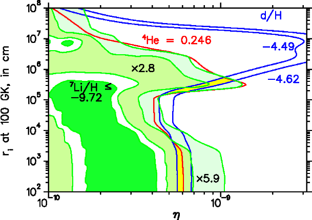
Figure 11: ( Color Online ) Observational constraints of ⁴He, deuterium, and ⁷Li are shown on the IBBN cylindrical shell model with $1-\sqrt{1-f_{v}}=$ 0.075, and $R_{\rho}=10^{6}$. The constraints $Y(^{7}{\mathrm{L}}{\mathrm{i}})/Y({\mathrm{p}})=1.23_{-0.32}^{+0.68}\times 10^{-10}$ Ryan et al. (2000) are shown. Also shown are ⁷Li constraints with depletion factors of 2.8 and 5.9.

Figure 11 shows the observational constraints from Figure 1 applied to the contour maps of Figures 3-5. The maximum $X_{{}^{4}{\mathrm{H}}{\mathrm{e}}}\leq$ 0.246 constraint from IT04 Izotov and Thuan (2004) and the ⁷Li constraints from Ryan et al Ryan et al. (2000) are shown in Figure 11.

Regions of concordance between the IT04 ⁴He maximum constraint and the deuterium constraints are shown in yellow. A concordance region exists for distance scales $r_{i}\leq$ 5000 cm and $\eta=(5.6-6.1)\times 10^{-10}$. These limits on $\eta$ are the same limits as seen in SBBN models. The maximum limit of $r_{i}$ is set by the shift to lower $\eta$ as neutron diffusion occurs closer to weak freeze-out. The $X_{{}^{4}{\mathrm{H}}{\mathrm{e}}}=$ 0.246 contour have a greater shift than the contour lines for the deuterium constraints, because of increased ⁴He production in the outer region.

Another region of concordance appears for $r_{i}=(1.3-6.0)\times 10^{5}$ cm, when the contour lines shift to higher $\eta$ due to the concentration of nucleosynthesis along the boundary. The upper cutoff of $r_{i}$ is determined by the condition when a trough as shown in Figure 9 exists in the ⁴He abundance distribution. Greater ⁴He production in the outermost shells cause the $X_{{}^{4}{\mathrm{H}}{\mathrm{e}}}=$ 0.246 contour to shift to lower $\eta$ while greater deuterium production in the trough cause the deuterium contour lines to remain shifted to higher $\eta$. The acceptable range of $\eta$ is $(4.3-12.0)\times 10^{-10}$, larger than in the SBBN case.

The ⁷Li constraints from Ryan et al Ryan et al. (2000) are shown in darkest green in Figure 11. The contour lines for ⁷Li tend to shift in the same direction with the contour lines of ⁴He and deuterium. So the ⁷Li constraints do not have a region of concordance with the ⁴He and deuterium constraints for this IBBN model, and the lack of a region of concordance persists for other geometries and parameter values. Figure 11 also shows the region of the ⁷Li constraints with a depletion factor of 2.8. That depletion factor would bring the ⁷Li constraints in concordance with the other isotopes for distances scales $r_{i}\leq$ 5000 cm. For the region of concordance corresponding to $r_{i}=(1.3-6.0)\times 10^{5}$ cm a larger depletion factor of 5.9 is needed. The greater production of ⁷Be shown in Figure 8 leads to the larger shift to lower $\eta$ in the ⁷Li contour lines compared to the ⁴He and deuterium contour lines, and the larger depletion factor. Figure 11 shows the region of the ⁷Li constraints with the depletion factor of 5.9. The benefit of IBBN models then is to allow for a larger range of ⁷Li depletion factor than permitted by the SBBN model.

Figure 11 is similar to Figure 2 from the proceedings article Lara 2004 Lara (2004). Differences between the figures include use of the newer $X_{{}^{4}{\mathrm{H}}{\mathrm{e}}}\leq$ 0.246 constraint Izotov and Thuan (2004) in place of the $X_{{}^{4}{\mathrm{H}}{\mathrm{e}}}\leq$ 0.248 constraint Olive et al. (2000). The method of calculating the diffusion coefficients Jedamzik and Rehm (2001) is also newer than the method Kurki-Suonio et al. (1992) used in Lara 2004. The neutron lifetime $\tau_{{\mathrm{n}}}=$ 885.7 seconds Eidelman and et al [ Particle Data Group ] (2004) was also updated for this article.

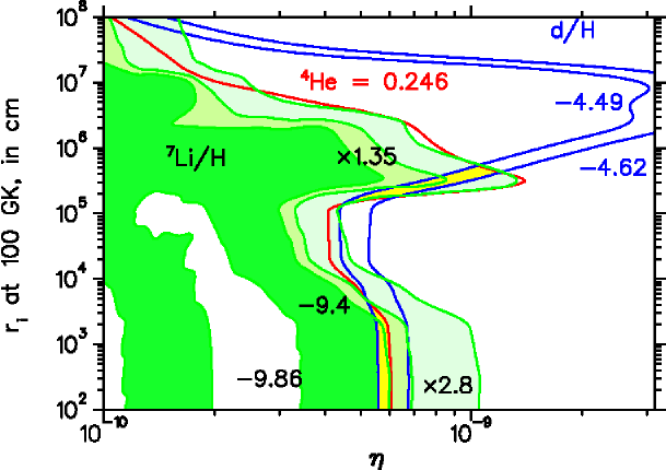
Figure 12: ( Color Online ) Same as in Figure 11, but showing the constraints $Y(^{7}{\mathrm{L}}{\mathrm{i}})/Y({\mathrm{p}})=2.34_{-0.96}^{+1.64}\times 10^{-10}$ Melendez and Ramirez (2004). Also shown are these constraints with depletion factors 1.35 and 2.8.

Figure 12 shows the ⁷Li constraints from Melendez & Ramirez Melendez and Ramirez (2004). The outermost edge of these $2\sigma$ constraints has concordance with most of the concordance region between ⁴He and deuterium for $r_{i}\leq$ 5000 cm. With a small depletion factor of 1.35 these ⁷Li constraints cover the whole region of concordance. A larger depletion factor of 2.8 is needed to cover the region of concordance corresponding to $r_{i}=(1.3-6.0)\times 10^{5}$ cm. The regions of concordance between ⁴He and deuteurium are controversial because of considerable disagreement regarding ⁴He constraints. Nonetheless both Figure 11 and Figure 12 show that Inhomogeneous Big Bang Nucleosynthesis allows for a larger range of acceptable ⁷Li depletion factor to bring deuterium and ⁷Li in concordance with each other, due to the greater shift in ⁷Li contour lines to lower $\eta$ for distance scales $r_{i}$ from $\approx$ 1600 cm to $10^{5}$ cm.

VI Conclusions

The Texas IBBN code is an original code written such that the weak and nuclear reactions of element synthesis are coupled with neutron diffusion. The time of neutron diffusion relative to the times of weak freeze-out and nucleosynthesis have a significant influence on the final production amounts of ⁴He, deuterium, and ⁷Li. Because diffusion is coupled to the reaction network the code correctly accounts for neutron back diffusion, wherein neutrons flow back into regions with higher proton density due to earlier nucleosynthesis in those regions. Back diffusion has an influence over the results especially when the time of neutron diffusion is close to the time of nucleosynthesis. Of most interest in the results is the larger range of depletion factor for ⁷Li that the IBBN model permits over the SBBN model.

In models where diffusion homogenizes the neutron distribution before weak freeze-out protons are coupled with the neutrons via the weak interconversion reactions. Protons are then redistributed. Proton redistribution is less effective in models with the time of diffusion closer to the time of weak freeze-out, leaving a higher proton density in the outer shells. Increasing proton density leads to earlier nucleosynthesis in the outer shells. Neutrons then back diffuse into the outer shells, concentrating nucleosynthesis there. Nucleosynthesis in the high density shells produces decreasing amounts of deuterium and increasing amounts of ⁴He and especially ⁷Be. The increased production of ⁷Be is significant in the determination of the depletion factor of ⁷Li.

For models with the time of diffusion close to the time of nucleosynthesis neutron back diffusion becomes less effective. Nucleosynthesis is concentrated in the volume fimmediately around the boundary. This concentration leads to decreasing ⁴He and ⁷Li+⁷Be production, and increasing deuterium production. In models where the time of neutron diffusion coincides with nucleosynthesis neutrons are not homogenized during nucleosynthesis. An increasing neutron number density remains in the outermost shells as well as a decreasing number density in the innermost shells. ⁴He, ⁷Li and ⁷Be production jumps in the high density outermost shells, and overall production of these isotopes increases. But between the boundary and the outermost shells are shells with a trough of low ⁴He production. Deuterium is produced in large amounts in that trough. The deuterium contour lines in Figure 4 diverge from the contour lines in Figures 3 and 4.

For models where neutron diffusion peaks at the same time as nucleosynthesis the trough in ⁴He production has disappeared. Deuterium production decreases and the deuterium contour lines in Figure 4 are in line with the lines in Figures 3 and 4. The divergence in the directions of contour lines is significant in setting constraints on $\eta$ and $r_{i}$ in the IBBN model.

Application of observational constraints to this IBBN model found slivers of concordance between the most recent deuterium constraints Kirkman et al. (2003) and ⁴He constraints by IT04 Izotov and Thuan (2004). Concordance occurs for $\eta=(5.6-6.1)\times 10^{-10}$ and $r_{i}\leq$ 5000 cm, and for $\eta=(4.3-12.3)\times 10^{-10}$ and $r_{i}=(1.3-6.0)\times 10^{5}$ cm. The point of divergence between the ⁴He and deuterium contour lines sets the maximum limit of acceptable $\eta$. The reliability of ⁴He constraints remains controversial Olive and Skillman (2004).

Contour lines between ⁴He, deuterium, and ⁷Li run roughly parallel to each other. The region Figure 11 marked by the ⁷Li constraints by Ryan et al Ryan et al. (2000) then does not have an overlap with the slivers of concordance of ⁴He and deuterium. A depletion factor of 2.8 would bring concordance in both the cases of SBBN and the first region of concordance. But because of the larger shift of the ⁷Li contour lines to lower $\eta$ a larger depletion factor of 5.9 is needed to bring the ⁷Li constraints in agreement with the second region of concordance. Recent ⁷Li constraints by Melendez & Ramirez Melendez and Ramirez (2004) have weak concordance with ⁴He and deuterium constraints in the SBBN case. But an IBBN model still allows for a larger range of depletion factor, up to 2.8, to have ⁷Li be in concordance with ⁴He and deuterium.

The IBBN abundance results for ⁷Li will be compared with new measurements of the ⁷Li primordial abundance derived from the ratio $(^{7}{\mathrm{L}}{\mathrm{i}}/^{6}{\mathrm{L}}{\mathrm{i}})$ measured in the InterStellar Medium Kawanomoto et al. (2003); Kawanomoto and et al. [ SUBARU/HDS Collaboration ] (2005). A new neutron lifetime $\tau_{{\mathrm{n}}}=878.5\pm 0.7\pm$ 0.3 seconds has recently been measured Serebrov and et al (2005). Constraints on $\eta$ in an SBBN model have been reassessed with the new lifetime Mathews et al. (2005), and the constraints on $\eta$ and $r_{i}$ in Figures 11 and 12 will also be reassessed with the new lifetime in an upcoming article Lara and et al. (2005). Additionally, this article will be followed up by articles applying an original solution of the neutrino heating effect Lara (2001a) to both SBBN and IBBN models.

VII Acknowledgements

This work was partially funded by National Science Foundation grants PHY 9800725, PHY 0102204, and PHY 035482. This author thanks the Center for Relativity at the University of Texas at Austin for the opportunity to work on this research, and Professor Richard Matzner in particular for his help in preparing this article. This author also thanks Professor Toshitaka Kajino of the National Astronomical Observatory of Japan for his advice on what to focus in this article.

Appendix A Trace of the Texas IBBN Code

The stretching function that sets the radii of the zones in the cylindrical shell model

$$\xi(r) = \xi(r_{b})+\frac{1}{C_{1}}\left(1-\frac{1}{C_{3}}\right)\sqrt{\frac{C_{2}}{C_{3}}}\arctan\left[(r-r_{b})\sqrt{\frac{C_{3}}{C_{2}}}\right]+\frac{r-r_{b}}{C_{1}C_{2}}$$ (2)

was used by KM90 Kurki-Suonio and Matzner (1990). The radius $r$ is normalized to equal 64 for the full radius of the model. Eq. 2 maps radii $r$ of the zone boundaries to unit values of $\xi$. Zones near $r_{b}$ have a width around $C_{1}$. Zones far from $r_{b}$ have widths determined by $C_{3}$ and a rate of zone-size change controlled by $C_{2}$. $r_{b}$ always corresponds to a unit value of $\xi$. For the model in this article there are 20 zones covering the high density outer shell and 44 covering the low density inner region. The baryon number densities $n_{b-high}$ in the outer shell’s zones and $n_{b-low}$ in the inner region’s zones are set

$$n_{b-low} = \frac{n_{b0}}{f_{v}R_{\rho}+(1-f_{v})}$$ (3)

$$n_{b-high} = R_{\rho}n_{b-low}$$ (4)

such that the number density averages out to $n_{b0}$ over the whole model.

At any given timestep the code solves the differential equation Mathews et al. (1990)

$$\frac{\partial n(i,s)}{\partial t} = n_{b}(s)\sum_{j,k,l}N_{i}\left(-\frac{Y^{N_{i}}(i,s)Y^{N_{j}}(j,s)}{N_{i}!N_{j}!}[ij]+\frac{Y^{N_{k}}(k,s)Y^{N_{l}}(l,s)}{N_{k}!N_{l}!}[kl]\right)$$ (5)

$$-3\dot{\alpha_{R}}n(i,s)+\frac{1}{r^{p}}\frac{\partial}{\partial r}\left(r^{p}D_{n}\frac{\partial\xi}{\partial r}\frac{\partial n(i,s)}{\partial\xi}\right)$$

for the number density $n(i,s)$ of isotope $i$ in zone $s$. The first two terms correspond to the weak and nuclear reactions that destroy ( $[ij]$ ) or create ( $[kl]$ ) isotope $i$ within zone $s$. $n_{b}(s)$ is the total baryon number density in zone $s$ and $Y(i,s)$ is the abundance $Y(i,s)$ of isotope $i$ in zone $s$.

$$Y(i,s) = \frac{n(i,s)}{n_{b}(s)}$$

The $3\dot{\alpha_{R}}n(i,s)$ term corresponds for the expansion of the universe, where $R$ is the expansion coefficient of the universe and $\alpha_{R}=\ln R$. This term can be eliminated by transforming to comoving coordinates. From here on $r$ will be in comoving coordinates. The last term corresponds to diffusion of isotope $i$ into and out of zone $s$. The factor $p$ depends on the geometry of the model. $p=$ 0 for planar symmetry, 1 for cylindrical symmetry and 2 for spherical symmetry. Currently only neutrons can diffuse in the Texas IBBN code. The neutron diffusion coefficient $D_{{\mathrm{n}}}$ is calculated from the coefficients $D_{{\mathrm{n}}{\mathrm{e}}}$ for neutron electron scattering and $D_{{\mathrm{n}}{\mathrm{p}}}$ for neutron proton scattering.

$$\frac{1}{D_{{\mathrm{n}}}} = \frac{1}{D_{{\mathrm{n}}{\mathrm{e}}}}+\frac{1}{D_{{\mathrm{n}}{\mathrm{p}}}}$$ (6)

Banerjee and Chitre Banerjee and Chitre (1991) derived a master equation for the diffusion coefficient between two particles scattering off of each other, based on the first order Chapman-Enskog approximation de Groot et al. (1980). Kurki-Suonio et al (KAGMBCS92) Kurki-Suonio et al. (1992), and Jedamzik and Rehm Jedamzik and Rehm (2001) derive the same equation for the diffusion coefficient $D_{{\mathrm{n}}{\mathrm{e}}}$ for neutron-electron scattering.

$$D_{{\mathrm{n}}{\mathrm{e}}} = \frac{3}{8}\sqrt{\frac{\pi}{2}}\frac{c}{n_{{\mathrm{e}}}\sigma_{{\mathrm{n}}{\mathrm{e}}}}\frac{K_{2}(z)}{\sqrt{z}K_{5/2}(z)}(1-\frac{n_{{\mathrm{n}}}}{n_{t}})$$ (7)

$K_{2}(z)$ and $K_{5/2}(z)$ are modified Bessel functions of order 2 and 5/2, $\sigma_{{\mathrm{n}}{\mathrm{e}}}$ is the transport cross section of the scattering and $z=m_{{\mathrm{e}}}/kT$. $n_{{\mathrm{n}}}/n_{t}$ is the neutron fraction of the total number of ALL particles. This fraction is of the order $10^{-10}$ and so can be ignored. For neutron-proton scattering Jedamzik and Rehm Jedamzik and Rehm (2001) derive an updated expression for the diffusion coefficient $D_{{\mathrm{n}}{\mathrm{p}}}$

$$D_{{\mathrm{n}}{\mathrm{p}}} = \frac{3}{8\sqrt{\pi}}\frac{c}{a_{s}^{2}}\frac{1}{n_{{\mathrm{p}}}}\sqrt{\frac{k_{B}T}{m_{N}c^{2}}}\frac{1}{I(a_{1},b_{1})+\frac{3a_{t}^{2}}{a_{s}^{2}}I(a_{2},b_{2})}$$ (8)

$$I(a,b) = \frac{1}{2}\int_{0}^{\infty}dx\frac{x^{2}e^{-x}}{ax+\left(1-\frac{bx}{2}\right)^{2}}$$

$$a_{1} = a_{s}^{2}\frac{m_{N}c^{2}}{\hbar^{2}c^{2}}k_{b}T$$

$$b_{1} = r_{s}a_{s}\frac{m_{N}c^{2}}{\hbar^{2}c^{2}}k_{b}T$$

$$a_{2} = a_{t}^{2}\frac{m_{N}c^{2}}{\hbar^{2}c^{2}}k_{b}T$$

$$b_{2} = r_{t}a_{t}\frac{m_{N}c^{2}}{\hbar^{2}c^{2}}k_{b}T$$

$m_{N}$ is the nucleon mass. The parameters $a_{s}=$ -23.71 fm, $r_{s}=$ 2.73 fm, $a_{t}=$ 5.432 fm, and $r_{t}=$ 1.749 fm come from singlet and triplet scattering.

The Texas IBBN code progresses a timestep $\Delta t_{m}$ for each step $m$. Eq. 5 is evolved using a implicit second order Runge-Kutta method Kawano (1992). To use this method, Eq. 5 has to be linearized. The weak-nuclear reaction terms can be linearized in a manner similar to the linearization of abundances $Y$ used by Wagoner Wagoner (1969) and this author Lara (1998).

$$\frac{n_{mA}(i,s)-n_{m-1}(i,s)}{\Delta t_{m-1}} = \sum_{j,k,l}-\frac{N_{i}[ij]}{N_{i}!N_{j}!(N_{i}+N_{j})}[N_{i}Y_{m}^{N_{i}-1}(i,s)Y_{m}^{N_{j}}(j,s)n_{mA}(i,s)+$$ (9)

$$N_{j}Y_{m}^{N_{i}}(i,s)Y_{m}^{N_{j}-1}(j,s)n_{mA}(j,s)]$$

$$+\frac{N_{i}[kl]}{N_{k}!N_{l}!(N_{k}+N_{l})}[N_{k}Y_{m}^{N_{k}-1}(k,s)Y_{m}^{N_{l}}(l,s)n_{mA}(k,s)+$$

$$N_{l}Y_{m}^{N_{k}}(k,s)Y_{m}^{N_{l}-1}(l,s)n_{mA}(l,s)]+\cdots$$

$\Delta t_{m-1}$ is the time difference between step $m-1$ and step $m$. For the diffusion term the zones are defined on a grid whose points $r(s)$ correspond to the outer radii of zones $s$. Number densities $n(i,s)$ are considered the number densities at the midpoint radius between the inner and outer radii of zone $s$. The points $r(s)$ correspond to points in $\xi(s)$ space a distance of one unit between each other. The first space derivative in the diffusion term in Eq. 5 can be discretized as:

$$\frac{\partial n}{\partial t} = \cdots\frac{1}{r^{p}}\frac{\partial}{\partial r}\left(r^{p}D\frac{\partial\xi}{\partial r}\frac{\partial n}{\partial\xi}\right)$$

$$\frac{\partial n}{\partial t} = \cdots\frac{1}{r^{p}}\frac{\partial}{\partial r}\left[\left(r^{p}D\frac{\partial\xi}{\partial r}\right)_{s-1/2}\frac{n[r(s)]-n[r(s-1)]}{1}\right]$$

Note that the coefficient $[r^{p}D(\partial\xi)/(\partial r)]$ depends on $r$. The $(1/r^{p})(\partial/\partial r)$ can be rewritten as a partial derivative of $r^{p+1}$. One can then write the discretization of the second space derivative as:

$$\frac{\partial n}{\partial t} = \cdots(p+1)\frac{\partial}{\partial(r^{p+1})}\left[\left(r^{p}D\frac{\partial\xi}{\partial r}\right)_{s-1/2}\frac{n[r(s)]-n[r(s-1)]}{1}\right]$$

$$\frac{\partial n}{\partial t} = \cdots(p+1)\left(\frac{\left(r^{p}D\frac{\partial\xi}{\partial r}\right)_{s}\{n[r(s+\frac{1}{2})]-n[r(s-\frac{1}{2})]\}}{r^{p+1}(s)-r^{p+1}(s-1)}\right.$$

$$\left.-\frac{\left(r^{p}D\frac{\partial\xi}{\partial r}\right)_{s-1}\{n[r(s-\frac{1}{2})]-n[r(s-\frac{3}{2})]\}}{r^{p+1}(s)-r^{p+1}(s-1)}\right)$$

For an isotope $i$ the densities $n[r(s+1/2)]$, $n[r(s-1/2)]$ and $n[r(s-3/2)]$ are defined as $n(i,s+1)$, $n(i,s)$ and $n(i,s-1)$ respectively. The coefficient $[r^{2}D(\partial\xi)/(\partial r)]_{s}$ is calculated at $r(s)$. One can apply this discretization to an implicit version of the diffision part of Eq. 5.

$$\frac{n_{mA}(i,s)-n_{m-1}(i,s)}{\Delta t_{m-1}} = \cdots-\frac{(p+1)\left(r^{p}D\frac{\partial\xi}{\partial r}\right)_{s}}{r^{p+1}(s)-r^{p+1}(s-1)}n_{mA}(i,s+1)$$ (10)

$$+(p+1)\frac{\left(r^{p}D\frac{\partial\xi}{\partial r}\right)_{s}+\left(r^{p}D\frac{\partial\xi}{\partial r}\right)_{s-1}}{r^{p+1}(s)-r^{p+1}(s-1)}n_{mA}(i,s)$$

$$-\frac{(p+1)\left(r^{p}D\frac{\partial\xi}{\partial r}\right)_{s-1}}{r^{p+1}(s)-r^{p+1}(s-1)}n_{mA}(i,s-1)$$

Any baryons that flow out beyond the distance scale are assumed to be replenished by baryons flowing in from other sets of shells, and $r(0)=$ 0 is the center of the shells. The code uses reflective boundary conditions at the endpoints of the grid.

$$\frac{n_{mA}(i,1)-n_{m-1}(i,1)}{\Delta t_{m-1}} = \cdots-\frac{(p+1)\left(r^{p}D\frac{\partial\xi}{\partial r}\right)_{1}}{r^{p+1}(1)-r^{p+1}(0)}n_{mA}(i,2)$$

$$+\frac{(p+1)\left(r^{p}D\frac{\partial\xi}{\partial r}\right)_{1}}{r^{p+1}(1)-r^{p+1}(0)}n_{mA}(i,1)$$

$$\frac{n_{mA}(i,64)-n_{m-1}(i,64)}{\Delta t_{m-1}} = \cdots+\frac{(p+1)\left(r^{p}D\frac{\partial\xi}{\partial r}\right)_{64}}{r^{p+1}(64)-r^{p+1}(63)}n_{mA}(i,64)$$

$$-\frac{(p+1)\left(r^{p}D\frac{\partial\xi}{\partial r}\right)_{63}}{r^{p+1}(64)-r^{p+1}(63)}n_{mA}(i,63)$$

where $r(64)=$ distance scale $r_{i}$. The above equations can be applied to the diffusion of any isotope $i$, but only neutrons ( $i=$ 1 ) diffuse for the results of this article.

Eq. 9 and Eq. 10 combined together can be rewritten as a matrix equation for a new number density value $n_{mA}(i,s)$. The matrix consists of a 68 $\times$ 68 matrix for each of the 64 zones, built from the terms in Eq. 9. From Eq. 10 come terms that couple $n(1,s)$ with $n(1,s+1)$ and $n(1,s-1)$ due to neutron diffusion. $n_{mA}(i,s)$ is then used in the following equation

$$\tilde{n}_{m}(i,s) = n_{m}(i,s)+\left[\frac{n_{mA}(i,s)-n_{m-1}(i,s)}{\Delta t_{m-1}}\right]\Delta t_{m}$$

to calculate an interim value $\tilde{n}_{m}(i,s)$ of the number densities. This is the first step of the Runge-Kutta method, with $\tilde{n}_{m}(i,s)$ the first estimate of the values of $n_{m}(i,s)$ at time $t_{m}+\Delta t_{m}$. Using $\tilde{Y}_{m}(i,s)=\tilde{n}_{m}(i,s)/\tilde{n}_{b}(s)$ the code solves a second matrix equation

$$\frac{n_{mB}(i,s)-n_{m}(i,s)}{\Delta t_{m}} = \sum_{j,k,l}-\frac{N_{i}[ij]}{N_{i}!N_{j}!(N_{i}+N_{j})}[N_{i}\tilde{Y}_{m}^{N_{i}-1}(i,s)\tilde{Y}_{m}^{N_{j}}(j,s)n_{mB}(i,s)+$$

$$N_{j}\tilde{Y}_{m}^{N_{i}}(i,s)\tilde{Y}_{m}^{N_{j}-1}(j,s)n_{mB}(j,s)]$$

$$+\frac{N_{i}[kl]}{N_{k}!N_{l}!(N_{k}+N_{l})}[N_{k}\tilde{Y}_{m}^{N_{k}-1}(k,s)\tilde{Y}_{m}^{N_{l}}(l,s)n_{mB}(k,s)+$$

$$N_{l}\tilde{Y}_{m}^{N_{k}}(k,s)\tilde{Y}_{m}^{N_{l}-1}(l,s)n_{mB}(l,s)]-$$

$$\frac{(p+1)\left(r^{p}D\frac{\partial\xi}{\partial r}\right)_{s}}{r^{p+1}(s)-r^{p+1}(s-1)}n_{mB}(i,s+1)$$

$$+(p+1)\frac{\left(r^{p}D\frac{\partial\xi}{\partial r}\right)_{s}+\left(r^{p}D\frac{\partial\xi}{\partial r}\right)_{s-1}}{r^{p+1}(s)-r^{p+1}(s-1)}n_{mB}(i,s)$$

$$-\frac{(p+1)\left(r^{p}D\frac{\partial\xi}{\partial r}\right)_{s-1}}{r^{p+1}(s)-r^{p+1}(s-1)}n_{mB}(i,s-1)$$

for new number density values $n_{mB}(i,s)$. $\Delta t_{m}$ is the time difference between step $m$ and step $m+1$. Final new values for $n_{m+1}(i,s)$ at timestep $m+1$ can then be calculated.

$$n_{m+1}(i,s) = n_{m}(i,s)+\frac{1}{2}\left[\frac{n_{mA}(i,s)-n_{m-1}(i,s)}{\Delta t_{m-1}}+\frac{n_{mB}(i,s)-n_{m}(i,s)}{\Delta t_{m}}\right]\Delta t_{m}$$ (11)

This is the second step ( “$B$” ) of the Runge-Kutta method. At the same time as with $n_{m}(i,s)$ the Texas IBBN evolves $\ln R$ and the electromagnetic plasma energy density $\rho_{{\mathrm{e}}+\gamma}$

$$\frac{d(\ln R)}{dt} = \sqrt{\frac{8}{3}\pi G(\rho_{\gamma}+\rho_{{\mathrm{e}}}+\rho_{\nu})}$$ (12)

$$\frac{d\rho_{{\mathrm{e}}+\gamma}}{dt} = -4\frac{\dot{R}}{R}\rho_{\gamma}-3\frac{\dot{R}}{R}(p_{{\mathrm{e}}}+\rho_{{\mathrm{e}}})$$ (13)

also by the Runge-Kutta method.

After both Runge-Kutta steps have been done the code determines the new baryon number density $n_{b}(s)$ of each zone using

$$n_{b}(s) = \sum_{i=1}^{68}A_{i}n(i,s)$$

where $A_{i}$ is the atomic weight of isotope $i$. From $n_{b}(s)$ and $n(i,s)$ the code can calculate $Y(i,s)$. At any given time the abundance $Y_{av}(i)$ and mass fraction $X_{i}$ of isotope $i$ in the entire model can be calculated from $Y(i,s)$ using

$$Y_{av}(i) = \frac{\sum_{s=1}^{64}n(i,s)[r^{p+1}(s)-r^{p+1}(s-1)]}{\sum_{s=1}^{64}n_{b}(s)[r^{p+1}(s)-r^{p+1}(s-1)]}$$

$$X_{i} = A_{i}Y_{av}(i)$$

These overall abundances and mass fractions can be shown as contour maps of the IBBN code’s parameters, and compared to observational constraints.

Figure 1: $X_{{}^{4}{\mathrm{H}}{\mathrm{e}}}$, $Y({\mathrm{d}})/Y({\mathrm{p}})$ and $Y(^{7}{\mathrm{L}}{\mathrm{i}})/Y({\mathrm{p}})$ for the SBBN case. The graph for $X_{{}^{4}{\mathrm{H}}{\mathrm{e}}}$ includes the measurements by IT04 ( Izotov and Thuan (2004) solid lines ) and by Luridinia et al ( Luridiana et al. (2003) dashed lines ). The graph for $Y(^{7}{\mathrm{L}}{\mathrm{i}})/Y({\mathrm{p}})$ shows measurements by both Ryan et al ( Ryan et al. (2000) solid lines ) and Melendez & Ramirez ( Melendez and Ramirez (2004) dashed lines ).

Figure 2: The stretching function will map integer values of $\xi$ to values of radius $r$ such that the $r$’s near the boundary radius $r_{b}$. are closely spaced. Here $r_{b}=$ 59.2.

Figure 3: The mass fraction $X_{{}^{4}{\mathrm{H}}{\mathrm{e}}}$ in the IBBN code. The horizontal axis is for baryon-to-photon ratio $\eta$ and the vertical axis is for distance scale $r_{i}$ in centimeters at temperature $T=$ 100 GK.

Figure 4: The log of abundance $Y({\mathrm{d}})/Y({\mathrm{p}})$

Figure 5: The log of abundance $Y(^{7}{\mathrm{L}}{\mathrm{i}})/Y({\mathrm{p}})$

Figure 6: Neutron diffusion vs. the interconversion reactions for $r_{i}\approx$ 25000 cm. The rate of diffusion from shell 63 to shell 62 is shown in solid while the greater rate from shell 62 to shell 61 is shown in long dashed lines. The net result of diffusion is neutron depletion in shell 62. The forward and reverse direction rates of the neutron to proton conversion reactions are shown in short dashed lines. Neutrons and protons are decoupled during the peak time of diffusion.

Figure 7: Back diffusion for $r_{i}\approx$ 25000 cm. The rate of diffusion from shell 62 to shell 63 is shown in solid while the greater rate from shell 61 to shell 62 is shown in long dashed lines. The direction of diffusion is now reversed, resulting in a net increase of neutrons in shell 62. Back diffusion coincides with the time when the nuclear reaction n + p $\leftrightarrow$ d + $\gamma$ ( shown in short dashed lines ) falls out of NSE.

Figure 8: The final number densities of ⁷Li and ⁷Be produced in each shell of the model, for $r_{i}\approx$ 25000 cm.

Figure 9: The final number density of ⁴He produced in each shell of the model. For $r_{i}\approx 3.2\times 10^{5}$ cm ⁴He production is concentrated surrounding the boundary. For $r_{i}=2\times 10^{6}$ cm ⁴He production has incresed in the outermost shells due to neutrons not homogenizing.

Figure 10: The final number density of deuterium produced in each shell of the model, for $r_{i}\approx 3.2\times 10^{5}$ cm and $r_{i}=2\times 10^{6}$ cm. Deuterium production remains considerably large in the trough of ⁴He production that arises in Figure 9.

References

- Smith et al. (1993) M. Smith, L. Kawano, and R. Malaney, Astrophys. J. Suppl. 85, 219 (1993).
- Steigman (2003) G. Steigman, in The Local Group as an Astrophysical Laboratory (STScI Symposium, 2003), astro-ph/0308511.
- Bennett and et al. (2003) C. Bennett and et al., Astrophys. J. Suppl. 148, 1 (2003).
- Lee and et al. (2001) A. Lee and et al., Astrophys. J. 561, L1 (2001).
- Jaffe and et al. (2001) A. Jaffe and et al., Phys. Rev. Lett. 86, 3475 (2001).
- Netterfield and et al. [ BOOMERanG Collaboration ] (2002) C. Netterfield and et al. [ BOOMERanG Collaboration ], Astrophys. J. 571, 604 (2002).
- Halverson and et al. (2002) N. Halverson and et al., Astrophys. J. 568, 38 (2002).
- Melchiorri (2002) A. Melchiorri (2002), astro-ph/0204262. Invited contribution to the 4th Heidelberg International Conference on Dark Matter in Astro- and Particle Physics.
- Hata et al. (1995) N. Hata, R. Scherrer, G. Steigman, D. Thomas, T. Walker, S. Bludman, and P. Langacker, Phys. Rev. Lett. 75, 3977 (1995).
- Copi et al. (1995) C. Copi, D. Schramm, and M. Turner, Phys. Rev. Lett. 75, 3981 (1995).
- Kernan and Sarker (1996) P. Kernan and S. Sarker, Phys. Rev. D 54, R3681 (1996).
- Hata et al. (1997) N. Hata, G. Steigman, S. Bludman, and P. Langacker, Phys. Rev. D 55, 540 (1997).
- Kainulainen et al. (1999) K. Kainulainen, H. Kurki-Suonio, and E. Sihvola, Phys. Rev. D 59, 083505 (1999).
- Skillman et al. (1994) E. Skillman, R. Televich, R. Kennicutt, D. Garnett, and E. Terlevich, Astrophys. J. 431, 172 (1994).
- Pagel (2000) B. Pagel, Phys. Rep. 333, 433 (2000).
- Olive and Skillman (2001) K. Olive and E. Skillman, New Astron. 6, 119 (2001).
- Esposito et al. (2000) S. Esposito, G. Mangano, G. Miele, and O. Pisanti, J. High Ergy. Phys 9, 38 (2000).
- Esposito et al. (2001) S. Esposito, G. Mangano, A. Melchiorri, G. Miele, and O. Pisanti, Phys. Rev. D 63, 043004 (2001).
- Kajino and Orito (1998) T. Kajino and M. Orito, Nucl. Phys. A 629, 538c (1998).
- Kajino (2002) T. Kajino, J. Nucl. Sci. & Tech. Supp. II, 530 (2002).
- Nollett and Lopez (2002) K. Nollett and R. Lopez, Phys. Rev. D 66, 063507 (2002).
- Ichiki et al. (2002) K. Ichiki, M. Yahiro, T. Kajino, M. Orito, and G. Mathews, Phys. Rev. D 66, 043521 (2002).
- Bratt et al. (2002) J. Bratt, A. Gault, R. Scherrer, and T. Walker, Phys. Lett. B 546, 19 (2002).
- Jedamzik and Rehm (2001) K. Jedamzik and J. Rehm, Phys. Rev. D 64, 023510 (2001).
- Kurki-Suonio and Sihvola (2001) H. Kurki-Suonio and E. Sihvola, Phys. Rev. D 63, 083508 (2001).
- Lara (1998) J. Lara, in Stellar Evolution and Stellar Explosions and Galactic Chemical Evolution, edited by A. Mezzacappa (Institute of Physics Publishing, 1998), p. 123, astro-ph/9806057.
- Izotov et al. (1994) Y. Izotov, T. Thuan, and V. Lipovetsky, Astrophys. J. 435, 647 (1994).
- Izotov et al. (1997) Y. Izotov, T. Thuan, and V. Lipovetsky, Astrophys. J. Suppl. 108, 1 (1997).
- Izotov and Thuan (1998) Y. Izotov and T. Thuan, Astrophys. J. 500, 188 (1998).
- Olive and Steigman (1995) K. Olive and G. Steigman, Astrophys. J. Suppl. 97, 49 (1995).
- Olive et al. (1997) K. Olive, G. Steigman, and E. Skillman, Astrophys. J. 483, 788 (1997).
- Peimbert et al. (2000) M. Peimbert, A. Peimbert, and M. Ruiz, Astrophys. J. 541, 688 (2000).
- Luridiana et al. (2003) V. Luridiana, A. Peimbert, M. Peimbert, and M. Cervino, Astrophys. J. 592, 846 (2003).
- Izotov and Thuan (2004) Y. Izotov and T. Thuan, Astrophys. J. 602, 200 (2004).
- Olive et al. (2000) K. Olive, G. Steigman, and T. Walker, Phys. Rep. 333, 389 (2000).
- Olive and Skillman (2004) K. Olive and E. Skillman, Astrophys. J. 617, 29 (2004).
- Kirkman et al. (2003) D. Kirkman, D. Tytler, N. Suzuki, J. O’Meara, and D. Lubin, Astrophys. J. Suppl. 149, 1 (2003).
- Tytler et al. (1996) D. Tytler, X. Fan, and S. Burles, Nature (London) 381, 207 (1996).
- Burles and Tytler (1998a) S. Burles and D. Tytler, Astrophys. J. 499, 699 (1998a).
- Burles and Tytler (1998b) S. Burles and D. Tytler, Astrophys. J. 507, 732 (1998b).
- Steigman (2001) G. Steigman, in Encyclopedia of Astronomy and Astrophysics (IoP Publishing, 2001), p. 1421, astro-ph/0009506.
- O’Meara et al. (2001) J. O’Meara, D. Tytler, D. Kirkman, N. Suzuki, J. Prochaska, D. Lubin, and A. Wolfe, Astrophys. J. 552, 718 (2001).
- Rugers and Hogan (1996) M. Rugers and C. Hogan, Astrophys. J., Lett. 459, 1 (1996).
- Ryan et al. (2000) S. Ryan, T. Beers, K. Olive, B. Fields, and J. Norris, Astrophys. J. 530, L57 (2000).
- Pinsonneault et al. (1999) M. Pinsonneault, T. Walker, G. Steigman, and V. Narayanan, Astrophys. J. 527, 180 (1999).
- Pinsonneault et al. (2002) M. Pinsonneault, G. Steigman, T. Walker, and V. Narayanan, Astrophys. J. 574, 398 (2002).
- Melendez and Ramirez (2004) J. Melendez and I. Ramirez, Astrophys. J. 615, L33 (2004).
- Lara (2001a) J. Lara, Ph.D. thesis, University of Texas at Austin (2001a).
- (49) J. Lara, http://www.ces.clemson.edu/~ljuan/work.html.
- Witten (1984) E. Witten, Phys. Rev. D 30, 272 (1984).
- Kurki-Suonio (1988) H. Kurki-Suonio, Phys. Rev. D 37, 2104 (1988).
- Ignatius and Schwarz (2001) J. Ignatius and D. Schwarz, Phys. Rev. Lett. 86, 2216 (2001).
- Malaney and Mathews (1993) R. Malaney and G. Mathews, Phys. Rep. 229, 147 (1993).
- Thomas et al. (1994) D. Thomas, D.N., Schramm, K. Olive, G. Mathews, B. Meyer, and B. Fields, Astrophys. J. 430, 291 (1994).
- Orito et al. (1997) M. Orito, T. Kajino, R. Boyd, and G. Mathews, Astrophys. J. 488, 515 (1997).
- Layek et al. (2001) B. Layek, S. Sanyal, and A. Srivastava, Phys. Rev. D 63, 083512 (2001).
- Layek et al. (2003) B. Layek, S. Sanyal, and A. Srivastava, Phys. Rev. D 67, 083508 (2003).
- Fuller et al. (1994) G. Fuller, K. Jedamzik, G. Mathews, and A. Olinto, Phys. Lett. B 333, 135 (1994).
- Heckler (1995) A. Heckler, Phys. Rev. D 51, 405 (1995).
- Rubakov and Shaposhnikov (1996) V. Rubakov and M. Shaposhnikov, Phys.–Uspehki 39, 461 (1996).
- Cline et al. (1998) J. Cline, M. Joyce, and K. Kainulainen, Phys. Lett. B 417, 79 (1998).
- Dolgov and Silk (1993) A. Dolgov and J. Silk, Phys. Rev. D 47, 4244 (1993).
- Nelson (1990) A. Nelson, Phys. Lett. B 240, 179 (1990).
- Zeldovich (1975) I. Zeldovich, Sov. Astr. Lett. 1, 5 (1975).
- Epstein and Petrosian (1975) R. Epstein and V. Petrosian, Astrophys. J. 197, 281 (1975).
- Barrow and Morgan (1983) J. Barrow and J. Morgan, Mon. Not. R. Astron. Soc. 203, 393 (1983).
- Applegate et al. (1987) J. Applegate, C. Hogan, and R. Scherrer, Phys. Rev. D 35, 1151 (1987).
- Alcock et al. (1987) C. Alcock, G. Fuller, and G. Mathews, Astrophys. J. 320, 439 (1987).
- Kajino and Boyd (1990) T. Kajino and R. Boyd, Astrophys. J. 359, 267 (1990).
- Kurki-Suonio et al. (1988) H. Kurki-Suonio, R. Matzner, J. Centralla, T. Rothman, and J. Wilson, Phys. Rev. D 38, 1091 (1988).
- Kurki-Suonio and Matzner (1989) H. Kurki-Suonio and R. Matzner, Phys. Rev. D 39, 1046 (1989).
- Kurki-Suonio et al. (1990) H. Kurki-Suonio, R. Matzner, K. Olive, and D. Schramm, Astrophys. J. 353, 406 (1990).
- Kurki-Suonio and Matzner (1990) H. Kurki-Suonio and R. Matzner, Phys. Rev. D 42, 1047 (1990).
- Mathews et al. (1990) G. Mathews, B. Meyer, C. Alcock, and G. Fuller, Astrophys. J. 358, 36 (1990).
- Mathews et al. (1996) G. Mathews, T. Kajino, and M. Orito, Astrophys. J. 456, 98 (1996).
- Lara (2001b) J. Lara, in The Seventh Texas-Mexico Conference on Astrophysics: Flows and Blows and Glows, edited by W. Lee and S. Torres-Peimbert (Revista Mexicana de Astronomia y Astrofisica, Serie de Conferencias, 2001b), p. 144, astro-ph/0101195.
- Lara (2004) J. Lara, in Frontier in Astroparticle Physics and Cosmology, edited by K. Sato and S. Nagataki, Research Center for the Early Universe (Universal Academy Press, 2004), p. 87, astro-ph/0402112.
- Eidelman and et al [ Particle Data Group ] (2004) S. Eidelman and et al [ Particle Data Group ], Phys. Lett. B 592, 1 (2004).
- Kurki-Suonio et al. (1992) H. Kurki-Suonio, M. Aufderheide, F. Graziani, G. Mathews, B. Banerjee, S. Chitre, and D. Schramm, Phys. Lett. B 289, 211 (1992).
- Kawanomoto et al. (2003) S. Kawanomoto, T.-K. Suzuki, H. Ando, and T. Kajino, Nucl. Phys. A 718, 659 (2003).
- Kawanomoto and et al. [ SUBARU/HDS Collaboration ] (2005) S. Kawanomoto and et al. [ SUBARU/HDS Collaboration ] (2005), in preparation for submittal to Astrophys. J. .
- Serebrov and et al (2005) A. Serebrov and et al, Phys. Lett. B 605, 72 (2005).
- Mathews et al. (2005) G. Mathews, T. Kajino, and T. Shima, Phys. Rev. D 71, 021302 (2005).
- Lara and et al. (2005) J. Lara and et al. (2005), in preparation for submittal to Phys. Rev. D.
- Banerjee and Chitre (1991) B. Banerjee and S. Chitre, Phys. Lett. B 258, 247 (1991).
- de Groot et al. (1980) S. de Groot, W. van Leeuwen, and C. van Weert, Relativistic Kinetic Theory (North-Holland, 1980).
- Kawano (1992) L. Kawano (1992), fermilab-Pub-92/04-A.
- Wagoner (1969) R. Wagoner, Astrophys. J. Suppl. 18, 247 (1969).