Mira Variables in the OGLE Bulge fields

The 222 000 $I$-band light curves of variable stars detected by the ogle-ii survey in the direction of the Galactic Bulge have been fitted and have also been correlated with the denis and 2mass all-sky release databases and with lists of known objects. Lightcurves, and the results of the lightcurve fitting (periods and amplitudes) and denis and 2mass data are presented for 2691 objects with $I$-band semi-amplitude larger than 0.45 magnitude, corresponding to classical Mira variables. The Mira period distribution of 6 fields at similar longitude but spanning latitudes from $-1.2$ to $-5.8$ are statistically indistinguisable indicating similar populations with initial masses of 1.5-2 M_⊙ (corresponding to ages of 1-3 Gyr). A field at similar longitude at $b=-0.05$ from Glass et al. (2001) does show a significantly different period distribution, indicating the presence of a younger population of 2.5-3 M_⊙ and ages below $1$ Gyr. The $K$-band period-luminosity relation is presented for the whole sample, and for sub-fields. The zero point depends on Galactic longitude. Simulations are carried out to show that the observed dependence of the zero point with $l$, and the number of stars per field are naturally explained using the model of disk and bulge stars of Binney et al. (1997), for a viewing angle (major-axis Bar - axis perpendicular to the line-of-sight to the Galactic Centre) of 43 $\pm$ 17 degrees. The simulations also show that biases in the observed zero point are small, $<0.02$ mag. A comparison is made with similar objects in the Magellanic Clouds, studied in a previous paper. The slope of the $PL$-relation in the Bulge and the MCs agree within the errorbars. Assuming the zero point does not depend on metallicity, a distance modulus difference of 3.72 between Bulge and LMC is derived. This implies a LMC DM of 18.21 for an assumed distance to the Galactic Centre (GC) of 7.9 kpc, or, assuming a LMC DM of 18.50, a distance to the GC of 9.0 kpc. From the results in Groenewegen (2004) it is found for carbon-rich Miras that the $PL$-relation implies a relative SMC-LMC DM of 0.38, assuming no metallicity dependence. This is somewhat smaller than the often quoted value near 0.50. Following theoretical work by Wood (1990) a metallicity term of the form $M_{\rm K}\sim\beta\log Z$ is introduced. If a relative SMC-LMC DM of 0.50 is imposed, $\beta=0.4$ is required, and for that value the distance to the GC becomes 8.6 $\pm$ 0.7 kpc (for a LMC DM of 18.50), within the errorbar of the geometric determination of 7.9 $\pm$ 0.4 kpc (Eisenhauer et al. 2003). An independent estimate using the absolute calibration of Feast (2004b) leads to a distance estimate to the GC of 8.8 $\pm$ 0.4 kpc.

1 Introduction

In the course of the micro lensing surveys in the 1990’s the monitoring of the Small and Large Magellanic Clouds has revealed an amazing number and variety of variable stars. A big impact was felt and is being felt in any area of variable star research, like Cepheids and RR Lyrae stars. Also in the area of variability in red variables (RVs) and AGB stars there has been remarkable progress. Wood et al. (1999) and Wood (2000) were the first to identify and label different sequences “ABC” thought to represent the classical Mira sequence (“C”) and overtone pulsators (“A,B”), and sequence “D” which is not yet satisfactorily explained (Olivier & Wood 2003, Wood et al. 2004. Stars on these sequence are referred to as having Long Secondary Periods–LSPs). This view has subsequently been confirmed and expanded upon by Noda et al. (2002), Lebzelter et al. (2002), Cioni et al. (2003), Ita et al. (2004) and Kiss & Bedding (2003, 2004), Fraser et al. (2005). These works differ in the source of the variability data (macho, ogle, eros, moa), area (SMC or LMC), associated infrared data (Siding Spring 2.3m, denis, 2mass, sirius), and selection on pulsation amplitude or infrared colours. In a recent paper, Groenewegen (2004; hereafter G04) analysed the ogle data in the SMC and LMC, and correlated these sources with the denis and 2mass surveys. The paper discussed the variability properties of three samples: about 2300 spectroscopically confirmed AGB stars, around 400 previously known LPV variables and about 570 candidate dust-obscured AGB stars.

The present paper is an extension of the analysis in G04 to the ogle data in the direction of the Galactic Bulge (GB). Also for this area of the sky, several papers exist that use the results of the micro lensing surveys and have extended previous classical works on Bulge variable stars, like those of Lloyd Evans (1976), Glass & Feast (1982), Whitelock et al. (1991), Glass et al. (1995; hereafter GWCF), Alard et al. (1996) and Glass et al. (2001).

Alard et al. (2001; herafter ABC01) correlated ISOGAL sources within the NGC 6522 and Sgr I Baade windows with the MACHO database and present a list of 332 stars with complete 4-band $V,R$ and [7],[15] magnitudes. Schultheis & Glass (2001) extended Alard et al. by also considering the denis and 2mass data in those fields in general, and for the variables in particular. Glass & Schultheis (2002; hereafter GS02) investigated a sample of 174 M-giants in the NGC 6522 Baade window and correlated them with denis  ISOGAL and MACHO. Many stars of spectral type M5 and all M6 and later show variation, whereas subtypes M1-M4 do not (see also Glass et al. 1999).

Glass & Schultheis (2003; hereafter GS03) investigated the variable stars in the NGC 6522 Baade’s window using MACHO data, and also used denis IR data. Of the 1661 selected stars 1085 were found to be variable. They present $K$-band $PL$-relations for sequences “ABCD”.

Wray et al. (2004) investigated small amplitude red giants variables in a sub-set of 33 ogle fields. They identified two groups that seem to correspond to groups “A-” and “B-” in Ita et al. (2004; also see G04).

In our paper we describe results on Mira variables selected from ogle Bulge fields. The paper is structured as follows. In Section 2 the ogle, 2mass and denis surveys are described. In Section 3 the model for the lightcurve analysis is briefly presented. In the remaining of the paper different results are described. The Period-Luminosity diagram is discussed in Section 5. A description of the Mira population in respect to the overall bulge population is given in Section 8. In Section 9 we show that the Miras are distributed in a bar-like structure and give the orientation. In the final section we give the distance to the Galactic Centre, based on the period-luminosity relation.

2 The data sets

The ogle-ii micro lensing experiment observed fourty-nine fields in the direction of the GB. Each field has a size 14.2′$\times$57′ and was observed in $BVI$, with an absolute photometric accuracy of 0.01-0.02 mag (Udalski et al. 2002). Table 4 lists the galactic coordinates of the field centers and the total number of sources detected in these fields.

Wozniak et al. (2002) present a catalog of about 222 000 variable objects based on the ogle observations covering 1997-1999, applying the difference image analysis (DIA) technique on the $I$-band data. The data files containing the $I$-band data of the candidate variable stars was downloaded from the ogle homepage (http://sirius.astrouw.edu.pl/^∼ogle/). According to Wozniak et al., the level of contamination by spurious detections is about 10%, but we presume this level is much less at the brighter magnitudes of the LPVs considered here. Table 4 lists the number of detected variable stars per field (Wozniak et al. 2002).

The denis survey is a survey of the southern hemisphere in $IJK_{\rm s}$ (Epchtein et al. 1999). The second data release available through ViZier was used (The DENIS consortium, 2003). The 221801 ogle objects were correlated on position using a 3″ search radius and 59894 matches were found.

The 2mass survey is an all-sky survey in the $JHK_{\rm s}$ near-infrared bands. On March 25, 2003 the 2mass team released the all-sky point source catalog (Cutri et al. 2003). The easiest way to check if a star is included in the 2mass database is by uplinking a source table with coordinates to the 2mass homepage. Such a table was prepared for the 221801 ogle objects and correlated on position using a 3″ radius. Data on 182361 objects were returned.

Table 1: First entries in the electronically available table, which lists: OGLE-field and number, the three fitted periods with errors and amplitude (0.00 means no fit), mean $I_{\rm ogle}$, and associated denis $IJK$ photometry with errors, and associated 2mass $JHK$ photometry with errors (99.9 and 9.99 means no association, or no value).

Table 2: First entries in the electronically available table, which list: OGLE-field and number, other names, spectral type and references. ISOGAL sources from the official catalog (OGA03) have the prefix “ISOGAL”. ISOGAL sources studied in OOS03 have the prefix “OOS03”. References in column 4 are given in the bibliography of the main text.

3 Lightcurve analysis

The model to analyse the lightcurves is described in detail in Appendices A-C in G04.

Briefly, a first code (see for details Appendix A in G04) sequentially reads in the $I$-band data for the 222 000 objects, determines periods through Fourier analysis, fits sine and cosine functions to the light curve through linear least-squares fitting and makes the final correlation with the pre-prepared denis and 2mass source lists. All the relevant output quantities are written to file.

This file is read in by the second code (see for details Appendix B in G04). A further selection may be applied (typically on period, amplitude and mean $I$-magnitude), multiple entries are filtered out (i.e. objects that appear in different ogle fields), and a correlation is made with pre-prepared lists of known non-LPVs and known LPVs or AGB stars. The output of the second code is a list with LPV candidates.

The third step (for details see Appendix C in G04) consists of a visual inspection of the fits to the light curves of the candidate LPVs and a literature study through a correlation with the simbad database. Non-LPVs are removed, and sometimes the fitting is redone. The final list of LPV candidates is compiled.

Details on the small changes in the codes w.r.t. the implementation in G04 are given in Appendix A of the present paper.

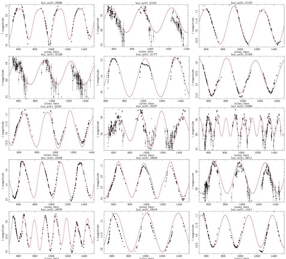
Figure 1: First entries of electronically available figure with all lightcurves. The fit is indicated by the (red) solid line. Crosses indicate data points not included in the fit.

4 Comparison of the datasets

4.1 Astrometry

As in G04, the correlation between the ogle objects and known LPVs and AGB stars, and known non-LPVs, is actually done in 2 steps. In the first step the correlation is made (for a 3″ search radius), and the differences and spread in $\Delta$RA $\cos(\delta)$ and $\Delta\delta$ are determined. These mean offsets are then applied in most cases to make the final cross-correlation, and this usually increases the number of matches. The results are listed in Table 3.

Table 3: Comparison of coordinates, and number of positional matches, before and after a correction was applied.

OGLE	$\Delta$RA $\cos(\delta)$	$\Delta\delta$	$N$	$\Delta$RA $\cos(\delta)$	$\Delta\delta$	$N$	remark
-(other)
IRAS	$0.14\pm$ 0.94	$0.50\pm$ 1.44	80				IRAS sources, not corrected
OGA03	$-0.80\pm$ 0.85	$-0.16\pm$ 0.89	1309	$-0.11\pm$ 0.82	$-0.02\pm$ 0.90	1319	ISOGAL sources from Omont et al. (2003; OGA03)
OOS03	$-0.80\pm$ 0.88	$-0.30\pm$ 0.95	800	$-0.10\pm$ 0.86	$-0.03\pm$ 0.99	817	ISOGAL sources from Ojha et al. (2003; OOS03)
GS02	$-0.02\pm$ 0.58	$0.30\pm$ 0.61	79	$-0.04\pm$ 0.67	$0.00\pm$ 0.61	80	MACHO sources from Glass & Schultheis (2002; GS02)
ABC01	$-0.82\pm$ 0.98	$-0.70\pm$ 0.96	293	$-0.17\pm$ 1.08	$-0.12\pm$ 1.01	320	ISOGAL sources from Alard et al. (2001; ABC01)
OGLE-I	$-0.08\pm$ 0.70	$-0.18\pm$ 0.44	728				ogle-i sources, not corrected
BMB	$-0.04\pm$ 0.70	$-0.52\pm$ 0.90	282	$+0.10\pm$ 0.79	$-0.08\pm$ 0.91	286	sources from Blanco et al. (1984; BMB)
TLE	$-0.08\pm$ 0.84	$-0.25\pm$ 1.43	21				sources from Lloyd-Evans (1976), not corrected
B84	$-0.46\pm$ 0.75	$0.50\pm$ 0.97	61	$-0.02\pm$ 0.76	$0.08\pm$ 1.05	63	sources from Blanco (1984; B84)

4.2 Photometry

As in G04, a comparison was made between the (mean) ogle $I$ and the (single-epoch) denis $I$, and between the (single-epoch) denis $JK$ and the (single-epoch) 2mass $JK$ magnitudes. This was done by selecting those objects with an amplitude in the $I$-band of $<0.05$ mag.

Figure 2 shows the final results when offsets $I$(denis-ogle) = $-0.03$, $J$(denis-2mass)= $-0.02$, and $K$(denis-2mass)= $-0.03$ are applied. The latter values are consistent with those derived in OOS03 based on the 2mass second incremental data release who found $J$(denis-2mass)= $-0.02\pm 0.09$, and $K$(denis-2mass)= $-0.00\pm 0.07$.

Figure 2: Difference in photometry, after the following offsets have been applied: $I$(denis-ogle) = $-0.03$, $J$(denis-2mass)= $-0.02$, $K$(denis-2mass)= $-0.03$.

5 Period-Luminosity relations

The full machinery outlined in Section 3 was performed. As in G04, all derived periods are given in Table 1 and are shown in Figure 1. The present paper discusses only objects which have at least one period with an $I$-band amplitude larger than 0.45 magnitudes, i.e. classical Mira variables (e.g. Hughes 1989). After visual inspection of the lightcurves a sample of 2691 such objects remain. The number of objects per field is listed in the last column of Tab. 4.

Table 1 lists the stars in the sample, the fitted periods with errors and amplitudes, and the denis and 2mass photometry of the associated sources. Table 2 lists alternative names and references from the literature. Figure 1 presents lightcurves and their fits.

In the discussion that follows, magnitudes are de-reddened using the $A_{\rm V}$ values that correspond to the respective ogle field taken from Sumi (2004; and $A_{\rm V}$ = 6.0 for the field 44 that they do not discuss), and selective reddenings of $A_{\rm I}/A_{\rm V}=0.49$, $A_{\rm J}/A_{\rm V}=0.27$, $A_{\rm H}/A_{\rm V}=0.20$, $A_{\rm K}/A_{\rm V}=0.12$ (Draine 2003) and implicitly assuming that all objects suffer this reddening value (i.e. ignoring differential reddening within a field, and ignoring that foreground and background objects would suffer a different reddening). Sumi’s method is based on the absolute magnitude of the Red Clump giants and is absolute calibrated using the $(V-K)$ colours of 20 RR Lyrae stars in Baade’s window. Popowski et al. (2003) present an extinction map (over 9000 resolution elements of 4x4 arc minute size) towards the GB based on MACHO $V,R$ photometry, under the assumption that colour-magnitude diagrams would look similar in the absence of extinction. For the centre of the ogle fields it was checked if there was a tile in the Popowski et al. set within 0.05 degrees distance. For those, the value of the visual extinction has been listed, next to the value in Sumi in Table 4. The rms difference $A_{\rm V}$ for the 21 field with values from both references is 0.18. Finally, Schultheis et al. (1999b) presented a reddening map for the inner GB comparing denis $J,K$ photometry to isochrones. Table 4 lists for two ogle fields the values they find: SC44 which was not considered by Sumi (2004), and SC5 for which Sumi derive a larger $A_{\rm V}$ than Schultheis et al.: 5.73 versus 4.13.

In the further discussion we only use periods that fulfil the following conditions are used in the calculations (with $\Delta P$ the error in the period): $\Delta P/P<0.01$ for $P<500^{d}$; $\Delta P<5^{d}$ for $500^{d}<P<800^{d}$ and $\Delta P<1.5^{d}$ for $P>800^{d}$. The latter constraint is necessary because the long periods become comparable to the length of the dataset.

Figure 3 shows the $K$-band $PL$-relation for all periods which have an $I$-band amplitude larger than 0.45 magnitude and $(J-K)_{0}<2.0$ among the 2691 stars. The cut in $(J-K)$ colour is needed to prevent that the $K$-magnitude is affected by circumstellar extinction, as shown in G04. Like G04, the $K$-magnitude is on the 2mass system, and is the average of the denis and 2mass photometry. In particular, if both denis and 2mass $K$-band data is available, the denis data point is corrected as explained above (i.e. 0.03 mag added), and averaged with the 2mass data point. This should take out some of the scatter in the $PL$-diagram, as the effect of the variability in the $K$-band is reduced. If only denis is available, the corrected value is used. In the left-hand panel the boundaries of the boxes “A-, A+, B-, B+, C, D” have been taken from G04, but shifted by $-4.0$ to account for the approximate difference in distance modulus (DM), as, e.g., follows from the recent determination of 7.9 $\pm$ 0.4 kpc (Eisenhauer et al. 2003) for the distance to the GC, and 18.50 for the DM to the LMC (e.g. recent reviews by Walker 2003, Feast 2004a).

There is a reasonably well defined sequence in Box “C”, but when compared to the similar figure for the SMC and LMC in G04 (his figure 3) some differences can be remarked as well. In particular, for the present Bulge sample there are a few objects located in Box “B+”, and in particular many in Box “D”. In the SMC and LMC, for this cut in amplitude, there are none in Box “B+” and few in “D”. Several issues may play a role. Applying a certain cut in amplitude may sample slightly different variables in SMC, LMC and Bulge. Figure 3 in G04 clearly shows how lowering the cut in amplitude results in a populating Box “B+” and then “A+”, and increases the number of objects in “D”. Another effect is the possible contribution of objects in the foreground and background of the Bulge, the depth of the Bulge, and fourthly, the orientation of the Bar, as the ogle fields span 20 degrees in longitude (this last effect will be discussed later). Finally, the difference in DM may be different from the adopted value of 4.0.

To verify if the objects in Box “D” actually show LSP, they were all visually inspected, and in fact few have, in agreement with the finding for LMC and SMC (for amplitudes $>$0.45 mag). This would call for a enlargement of Box “C” to properly sample the $PL$-relation of the large amplitude (Mira) variables. To define this enlarged box the $PL$-relation was inspected for each field independently. The right-hand panel in Figure 3 shows the finally adopted boundaries of Box “C”, which implies that Box “D” has contracted. Stars inside this redefined Box will be used to define the $PL$-relation. The $K$-band $PL$-relation is determined to be:

$$m_{\rm K}=(-3.37\pm 0.09)\;\log P+(15.44\pm 0.21)$$ (1)

with an rms of 0.42 and based on 1292 stars, and is shown in Fig. 3. The value of the slope is consistent with the median value when the $PL$-relation is determined for all fields individually.

For reference, fitting all stars in Figure 3, for a fixed slope of $-3.37$ results in a ZP of 15.47 $\pm$ 0.55.

Table 4: Properties of the ogle-fields

BUL_SC	$l$	$b$	Total(a)	Variable(b)	$A_{\rm V}$(c)	LPV(d)
1	1.08	-3.62	730	4597	1.68 / 1.49	42
2	2.23	-3.46	803	5279	1.55 / 1.65	48
3	0.11	-1.93	806	8393	2.89	115
4	0.43	-2.01	774	9096	2.59 / 2.94	86
5	-0.23	-1.33	434	7257	5.73 / – / 4.13	118
6	-0.25	-5.70	514	3211	1.37	47
7	-0.14	-5.91	463	1618	1.33 / 1.28	21
8	10.48	-3.78	402	2331	2.14	8
9	10.59	-3.98	330	1847	2.08	21
10	9.64	-3.44	458	2499	2.23	16
11	9.74	-3.64	426	2256	2.27	18
12	7.80	-3.37	535	3476	2.29 / 2.20	33
13	7.91	-3.58	570	3084	2.06 / 1.82	21
14	5.23	2.81	619	4051	2.49	51
15	5.38	2.63	601	3853	2.77	71
16	5.10	-3.29	700	4802	2.15 / 2.23	45
17	5.28	-3.45	687	4690	1.94 / 2.29	167
18	3.97	-3.14	749	5805	1.83	55
19	4.08	-3.35	732	5255	2.74	51
20	1.68	-2.47	785	5910	1.94 / 2.02	64
21	1.80	-2.66	883	7449	1.83 / 1.78	60
22	-0.26	-2.95	715	5589	2.74	70
23	-0.50	-3.36	723	4815	2.70	60
24	-2.44	-3.36	612	4304	2.52	56
25	-2.32	-3.56	622	3046	2.34	61
26	-4.90	-3.37	728	4713	1.86	39
27	-4.92	-3.65	691	3691	1.69	46
28	-6.76	-4.43	406	1472	1.64	16
29	-6.64	-4.62	492	2398	1.53	36
30	1.94	-2.84	762	6893	1.91 / 1.78	50
31	2.23	-2.94	790	4789	1.81 / 1.74	59
32	2.34	-3.14	797	5007	1.61 / 1.82	54
33	2.35	-3.66	739	4590	1.70 / 1.82	105
34	1.35	-2.40	961	7953	2.52 / 2.32	60
35	3.05	-3.00	771	5169	1.84 / 2.20	39
36	3.16	-3.20	873	8805	1.62 / 1.52	38
37	0.00	-1.74	664	8367	3.77	108
38	0.97	-3.42	710	5072	1.83 / 1.94	57
39	0.53	-2.21	784	7338	2.63 / 2.70	99
40	-2.99	-3.14	631	4079	2.94	55
41	-2.78	-3.27	603	4035	2.65	49
42	4.48	-3.38	601	4360	2.29	32
43	0.37	2.95	474	3351	3.67	112
44	-0.43	-1.19	319	7836	6.0 / – / 6.00	132
45	0.98	-3.94	627	2262	1.64 / 1.53	32
46	1.09	-4.14	552	2057	1.71 / 1.65	26
47	-11.19	-2.60	301	1152	2.60	12
48	-11.07	-2.78	287	973	2.35	12
49	-11.36	-3.25	251	826	2.09	18
total			30490	221701		2691

(a) Total number of objects detected in the field. From Udalski et al. (2002), in units of $10^{3}$ objects

(b) Total number of candidate variable stars. From Wozniak et al. (2002).

(c) Visual extinction. From Sumi (2004), except for SC44, where $A_{V}$ = 6.0 has been adopted based on the proximity to SC5. The second value–when listed–comes from Popowski et al. (2003). The third value–when listed–comes from Schultheis et al. (1999b).

(d) Total number of LPVs.

Figure 3: $K$-band $PL$-relation for periods with an $I$-band amplitude larger than 0.45 mag and $(J-K)_{0}<2.0$. Left panel: Sequences/Boxes “A+, A-, B+, B-, C, D” taken from G04 for the LMC and shifted by -4.0 in distance modulus. Right panel: enlarged Box “C” (and contracted Box “D”,) to define the region for which the $PL$-relations will be computed. Only periods from Table 1 that fulfil $\Delta P/P<0.01$ for $P<500^{d}$; $\Delta P<5^{d}$ for $500^{d}<P<800^{d}$ and $\Delta P<1.5^{d}$ for $P>800^{d}$ are plotted and used in the analysis. known M-stars are indicated by open circels. The line in the right-hand panel indicates the $PL$-relation of Equation 1.

6 Historical versus current periods

Table 5 compares the period derived in the present paper (the one with the largest amplitude) with values derived in the literature. There are three cases where a previously determined period may be a harmonic of the present period but overall there is good agreement between periods. In the 12 cases where there is a period available from LE76 (with the photographic plates taken between 1969 and 1971, hence 28 years of time difference with ogle) there is no clear case for a star that changed period. By comparison, G04 found that about 8% of LMC variables changed their period by more than 10% over a about 17 year timespan. To find 0 out of 12 in the present sample is consistent with this.

Table 5: Current Period compared to values listed in the literature

OGLE-name	Periods	Remark
bul_sc01_0558	232.2 (OGLE-II), 217.0, Mira (OGLE-I)
bul_sc01_1467	519.3 (OGLE-II), 265.0, Mira (OGLE-I)	harmonic ?
bul_sc01_1738	458.0 (OGLE-II), 227.5, Mira (OGLE-I)	harmonic ?
bul_sc01_2079	524.7 (OGLE-II), 520.0, Mira (OGLE-I)
bul_sc20_0832	245.9 (OGLE-II), 254.1: (ABC01), 235 (LE76), 336 (GWCF)
bul_sc20_0975	167.7 (OGLE-II), 145.8 (ABC01)
bul_sc20_1189	220.0 (OGLE-II), 121.3 (ABC01)	harmonic ?
bul_sc20_1292	87.7 (OGLE-II), 88.1 (ABC01)
bul_sc20_1761	231.6 (OGLE-II), 107.9 (ABC01), 240 (LE76), 235 (GWCF)
bul_sc20_1826	331.7 (OGLE-II), 330: (LE76)
bul_sc20_1928	297.6 (OGLE-II), 300 (LE76), 293 (GWCF)
bul_sc20_2013	453.3 (OGLE-II), 474.2: (ABC01), 500:: (LE76), 480 (GWCF)
bul_sc20_2269	409.3 (OGLE-II), 400: (LE76), 383 (GWCF)
bul_sc20_2291	311.2 (OGLE-II), 306.9: (ABC01), 315 (LE76), 308 (GWCF)
bul_sc34_3759	289.8 (OGLE-II), 293.8 (ABC01), 265 (LE76), 237 (GWCF)
bul_sc45_0704	405.3 (OGLE-II), 430 (LE76), 467, Mira (OGLE-I), 413 (GS03)
bul_sc45_1068	115.2 (OGLE-II), 115 (LE76), 116 (GCVS), 116 (GS03)
bul_sc45_1586	193.3 (OGLE-II), 190 (LE76), 195 (GS03)
bul_sc46_0866	322.1 (OGLE-II), 305 (LE76), 320 (GS03)
bul_sc46_1163	343.7 (OGLE-II), 329.0, Mira (OGLE-I)

7 Colour-colour diagrams

The 2mass and denis Colour-colour and colour-magnitude diagrams are shown in Fig. 4, together with that of spectroscopically confirmed M-stars in the LMC (see also Figure 12 in G04). There appear to be more redder stars in the Bulge sample, but this is likely due to a under representation in the LMC sample as this was restricted to spectroscopically known M-stars (i.e. in general optically selected). The sample of candidate infrared-selected AGB stars in the LMC [Figure 12 in G04] does cover the $(I-K)$ and $(J-K)$ colour range observed in the Bulge).

The other main difference is that the Bulge stars are redder by $\sim 2$ mag in $(I-J)_{0}$ compared to both LMC and SMC stars, as was also shown by Lebzelter et al. (2002) in a comparison of LMC and Bulge variable stars. As the diagrams involving $J,H,K$ colours appear similar, it seems that this difference in $(I-J)$ must be due to a difference in $I$. The $I$-band measurements of M stars is strongly affected by the TiO and VO molecular absorption features (Lançon & Wood 2000). It is expected that for larger metallicities these lines will be stronger (Schultheis et al. 1999a) which will lead to redder $(I-J)$ colours.

The bullets connected by a line in the Bulge denis $(I-J)-(J-K)$ colour-colour diagram are the average colours of M1, M2, .., M6, M6.5, M7, M8 giants in the NGC 6522 Baade’s window (Blanco 1986, GS02). There is a spread of typically 0.3-0.5 mag in $(I-J)$ and 0.2-0.3 mag in $(J-K)$ around these means, and there is only 1 M8 giant in their sample. The colours of the Miras follow those of normal giants well until M6.5, when the Miras become redder in $(I-J)$.

There are also stars redder in $(J-K)$ than the single M8 star in the sample of GS02, indicating either the presence of later spectral types or the on-set of circumstellar reddening.

The conclusion of GS02 that “Many M5 and all stars M6 and later show variation, whereas subtypes (M1-M4) do not” is confirmed here, as there are essentially no objects located in the region of the denis $(I-J)-(J-K)$ colour-colour diagram occupied by spectral types of M4 and earlier.

Figure 4: Colour-Magnitude and colour-colour diagrams using 2mass and denis photometry for the Bulge stars (left), and spectroscopically confirmed M-stars in the LMC (right, from G04). The bullets connected by a line in the Bulge DENIS $(I-J)-(J-K)$ diagram are the average colours of M1, M2, .., M6, M6.5, M7, M8 giants in the NGC 6522 Baade’s window (Blanco 1986, Glass & Schultheis 2002).

8 Mira bulge population as function of latitude

Figure 5 shows the period distribution of Miras in Box “C”. A distinction is made between all Miras and those with $(J-K)_{0}<2.0$ (dashed histograms). The latter selection minimises any influence of circumstellar extinction. For comparison, the period distribution of LMC and SMC Miras is also shown. The Kolmogorov-Smirnov (KS) test is performed to indicate that the probability that the period distributions of Bulge-LMC, Bulge-SMC, LMC-SMC are the same for all stars (those with $(J-K)_{0}<2$, respectively) is, respectively 0.36 (10^-8), 0.05 (0.31) and 0.05 (0.05).

Any difference, in particular between Bulge and LMC period distribution, is difficult to quantify further as this depends in a complicated way on the Star Formation History and evolutionary tracks ($T_{\rm eff}$ - Luminosity - Mass - metallicity). Regarding the period distribution of Bulge Miras as such, previous studies are limited to selected small fields (e.g. TLE, GWCF, Glass et al. 2001). Whitelock et al. (1991) present the period distribution of about 140 IRAS sources but no direct comparison is possible because of the difference in the selection criteria of the samples.

Figure 6 shows the period distribution of selected fields with very similar longitudes that cover a range in latitudes (the stars with $(J-K)_{0}<2.0$ are shown as dashed histogram again). To add a field even closer to the GC than surveyed by ogle the data in Glass et al. (2001, 2002) is considered on a field centered on $l=-0.05,b=-0.05$. They present the results of a $K$-band survey of 24 $\times$ 24 arcmin² for LPVs down to $K\sim 12.0$. From the list of 409 stars, 14 were removed because of double entries, quality index of zero, uncertain or no listed period or amplitude. The coordinates were uploaded to the IPAC webserver and 2mass data within 2.5″ was retrieved for these 395 stars to get information on the $(J-K)$ colour. As an additional check, and to eliminate multiple stars within the search circle, it was verified that the single-epoch 2mass $K$ magnitude is consistent with the mean $K$-magnitude and amplitude listed in Glass et al. For 345 stars 2mass data is available. The magnitudes are corrected for interstellar reddening using the extinction map of the inner GB at 2′ resolution by Schultheis et al. (1999b). The extinction value of the nearest available grid point in this map is taken. The extinction values range between 18.5 and 30.4 with a mean of 24.7. The top panel in Figure 6 list 333 stars with $K>7$ (to eliminate 3 very likely foreground objects), and $K$-band amplitude larger than 0.35 (to correspond roughly to the cut in $I$-band amplitude of 0.45 mag), and 88 (the histogram with slanted hatching), or 236 (dashed histogram) stars which also have $(J-K)_{0}<2.0$. The latter sample is the one that results when the reddening values from Schultheis et al. are multiplied by 1.35. They mention themselves that the reddening may be underestimated in the direction of the GC because of $J$-band non-detections. For the one field in common, their value is a factor 1.3-1.4 smaller than derived by Sumi (2004). In addition, for their default reddening (the histogram with slanted hatching in Figure 6) there would be many stars even at periods shorter than about 250 days which still would have $(J-K)_{0}>2.0$ which is not observed in the other fields. This could off course be real, but it is generally believed (e.g. Launhardt et al. 2002) that the population of low- and intermediate mass stars in the Nuclear Bulge (the inner about 30 pc from the GC) and GB are similar, but that in the former there is an overabundance of $10^{7}-10^{8}$ year old stars. In this picture one would expect the period distributions to be similar at shorter periods, essentially independent of latitude. Therefore the period distribution of stars with $(J-K)_{0}<2.0$ for the increased reddening is adopted.

The KS test is performed on consecutive fields in latitude for the distributions based on the stars with $(J-K)_{0}<2.0$. It is found that the probability that the distributions are the same is $10^{-10}$ for the $b=-0.05/$ $-1.21$ fields, 0.50 for the $b=-1.21/$ $-1.39$ fields, 0.80 for the $b=-1.39/$ $-1.81$, and $>0.99$ for the fields at more negative latitudes. The conclusion is that the period distributions of the fields at and below $-1.2$ degree are statistically indistinguisable, but that the field at $-0.05$ latitude has a significantly different period distribution (the probability that this distribution is the same as the distribution of the combined 6 ogle fields is $10^{-22}$). This conclusion is independent of the assumed reddening of the inner Bulge field, which influences how many stars will have $(J-K)_{0}<2.0$. For the default reddening of Schultheis et al., the probability that the distributions are the same for the $b=-0.05/$ $-1.21$ fields is still only 0.0033. The difference in the period distributions is especially clear at longer periods. Of the 236 stars in the inner field with $(J-K)_{0}<2.0$ 61 have $P>500$ days, while in the other fields this is 3 out of 367.

The difference in period distribution might be due to an under representation of short period stars in the inner field. However, Figure 4 in Glass et al. illustrates that the expected $K$-magnitudes at short periods are not fainter than the completeness limit of their survey. In fact, Glass et al. mention that they expect that the number of short-period Miras ($P<250$ days) is at least 75% complete. As a test, one-third of stars with $P<250$ days were randomly duplicated and added to the sample, and the KS test repeated to find again a large difference between the period distribution of the field at $-0.05$ degrees and the other fields.

The difference is emphasised in Figure 7 where the scaled period distribution of stars which have $(J-K)_{0}<2.0$ in the 5 fields between $b=-1.39\degr$ and $b=-5.8\degr$ has been subtracted from the inner field. The scaling was done in such a way that at shorter periods the two distributions would cancel at a level of 1$\sigma$ (based on Poisson errors). Even if the scaling is done in a slightly different way the result is always very similar, in the sense that there is a significant ($>4\sigma$) overabundance of LPVs in the inner field bewteen about 350 and 600 days.

The conclusion is that there is a significant population of LPVs with period $\raisebox{-3.1298pt}{$\stackrel{{\scriptstyle>}}{{\sim}}$}500$ days present in the inner field, which remains barely present at latitude $-1.2\degr$, and is absent for $b\raisebox{-3.1298pt}{$\stackrel{{\scriptstyle<}}{{\sim}}$}-1.4\degr$. This was indirectly noted by Glass et al. who noticed that the average period of the stars in this field at $b=-0.05\degr$ is 427$d$ (and that of the known OH/IR stars 524$d$), while the average period in the Sgr i window ($b=-2.6\degr$) is 333$d$, with no known OH/IR stars (GWCF).

To quantify the nature of the Mira Bulge population, synthetic AGB evolutionary models have been calculated, which are described in detail in Appendix C.

In brief, the synthetic AGB code of Wagenhuber & Groenewegen (1998) was finetuned to reproduce the models of Vassiliadis & Wood (1993) and then extended to more initial masses and including mass loss on the RGB. For several initial masses the fundamental mode period distribution was calculated for stars inside the observed instability strip and when the mass loss was below a critical value to simulate the fact that they should be optically visible. Vassiliadis & Wood (1993) provide calculations for 4 different metal abundances: $Z=0.016,0.008,0.004$ and 0.001. We used the models for $Z=0.016$, representing a solar mix, which are most appropriate for our Bulge sample (e.g. Rich 1998). We also show that our results are essentially unchanged if $Z$ = 0.01 or 0.02 are adopted. From the comparison of the observed period distribution for fields more than $1.2\degr$ away from the galactic centre with the theoretical ones, we deduce that the periods can be explained with a population of stars with Main Sequence masses in the range of 1.5 to 2.0 M_⊙. A possible extension to smaller masses is possible, but not necessary to explain the periods below 200 days. To explain the excess periods in the range of 350-600 days observed closer to the centre we need initial masses in the range 2.5 - 3 M_⊙. The presence of more massive stars in the inner field at $b$ = $-0.05\degr$ cannot be excluded, as it turns out that for more massive stars the optically visible Mira phase is essentially absent. Sevenster (1999) analysed OH/IR stars (which are LPVs with longer periods and higher mass loss rates than the Miras) in the inner Galaxy and came to the conclusion that OH/IR stars in the bulge have a minimum intial mass of about 1.3 M_⊙, based on an analysis of infrared colours, compatible with our results. We briefly mention here the result from Olivier et al. (2001) who studied a sample of LPVs in the solar neighbourhood with periods in the 300 to 800 days range. They conclude that majority of these stars had initial masses in the range of 1 - 2 M_⊙, with an average value of 1.3 M_⊙, lower than what we find for the 300 to 600 days range sample. This difference may be explained by the fact that our conclusions are only valid for a sample with no or only low mass loss rates ($\raisebox{-3.1298pt}{$\stackrel{{\scriptstyle<}}{{\sim}}$}5\times 10^{-6}\leavevmode\nobreak\ \mbox{M${}_{\odot}$}/yr$ ), contrary to their sample which was selected to contain stars with significant mass loss ($\sim 10^{-5}\leavevmode\nobreak\ \mbox{M${}_{\odot}$}/yr$). As can be seen in the Vassiliadis & Wood (1993) models, the period increases considerably when the stellar mass is reduced by the mass loss process.

We do not see a variation in the period distributions for the higher latitude fields (beyond $1\degr$ latitude) and can consider this as a homogeneous “bulge” population, which according to the Vassiliadis & Wood (1993) model has ages in the range of 1 to about 3 Gyr. The excess population closer to the Galactic Centre is younger than 1 Gyr. According to Launhardt et al. (2002), the Nuclear Bulge (approximately the central degree) contains besides the bulge population seen at higher latitudes also an additional population due to recent star formation closer to the galactic centre. Blommaert et al. (1998) find that the extrapolation of the number density of bulge OH/IR stars towards the galactic centre would explain half of the galactic centre OH/IR population, but that an additional population, intrinsic to the galactic centre, exists which agrees with what we see in the distribution here.

The formation history of the Bulge is still a matter of debate. In several works like in Kuijken & Rich (2002) and recently in Zoccali et al. (2004), the bulge is considered to be old ($>10$ Gyr) and formed on a relatively short timescale ($<1$ Gyr) (e.g. Ferreras et al. 2003). On basis of the modelling of colour-magnitude diagrams, Zoccali et al. claim that no trace is found of any younger stellar population than 10 Gyr. The bulge Miras do not fit in this picture as, according to our analysis, they are considerably younger. The field studied by Zoccali et al. is centered at ($l,b$) = (0.277, $-6.167$) so at a slighter higher latitude than our extreme fields ($b\approx-5.8\degr$). Although we are limited by the small number of Miras detected at the highest latitude fields, we do not see a change in period distribution for those fields. Zoccali et al. (2004) acknowledge the presence of Miras, but consider them as part of the old population. It is true that Miras are also detected in globular clusters and thus can be associated with old ages, as is the case for a 1 M_⊙ star in the Vassiliadis & Wood (1993) model but these stars produce periods shorter than 200 days (Figure C.1), insufficient to explain the period distribution seen in the bulge. The periods of Miras in Globular Clusters range from 150 to 300 days (Frogel & Whitelock 1998) and so only overlap with the shorter periods of the bulge Miras.

Our results agree more with the analysis of the infrared ISOGAL survey discussed in van Loon et al. (2003). They conclude that the bulk of the bulge population is old (more than 7 Gyr) but that a fraction of the stars is of intermediate age (1 to several Gyr). The Miras in our study can thus be considered as the intermediate age population seen in their analysis. van Loon et al. also see evidence for an even younger population ($<200$ Myr), but according to our findings, this would be restricted to the area close to the Galactic Centre.

Our discussion on the ages of the Mira stars is based on the assumption that they have evolved from single stars. An alternative scenario as suggested by Renzini & Greggio (1990), would be that the brighter (longer period) Miras could evolve from close binaries where the components coalesced to form one single star. This could lead to an underestimation of the age as the Mira essentially is the product of lower mass and thus older stars. This scenario may seem in better agreement with the idea that the bulge consists of an old stellar population. It however suffers from the same problem as the intermediate age population, in the sense that also no clear evidence for Blue Stragglers (which would be the Main Sequence counterpart of the Miras) is found (Kuijken & Rich, 2002).

If indeed the bulk of the bulge population is old and formed quickly and if the Miras are of intermediate age, then our Miras must be representatives of a population which was added at a later stage and it is unclear how it relates to the overall bulge. An interesting scenario suggested in Kormendy & Kennicutt (2004) is the one in which a secondary bulge or also called pseudo-bulge forms within an old bulge. Such a process would be connected to the presence of a “bar” which would add “disky” material into the old classical bulge. The Miras are indeed situated in a bar-structure as is discussed in the following section.

Figure 5: Period distribution of large amplitude variables in box “C”, for Bulge (top), LMC (middle), and SMC (bottom). For the shaded histogram only stars with $(J-K)_{0}<2.0$ have been included.

Figure 6: Mira period distribution for 7 fields with similar longitudes but a range in latitudes (as indicated in the top right corner). For the field at $b\sim-5.8\degr$, ogle fields 6 and 7 have been combined. For the shaded histograms only stars with $(J-K)_{0}<2.0$ have been included. The field at $(-0.05,-0.05)$ is based on Glass et al. (2001), see main text for details. The histogram with slanted hatching is for the reddening by Schultheis et al. (1999b) for stars in this field, the shaded histogram for the adopted reddening which is 1.35 times larger.

Figure 7: Period distribution of the stars in the $b=-0.05\degr$ field with $(J-K)_{0}<2.0$ minus the suitably scaled period distribution of the stars in the $b=-1.39$ to $-5.8\degr$ fields with $(J-K)_{0}<2.0$. The scaling is such that below $\stackrel{{\scriptstyle<}}{{\sim}}$300 days the two distributions cancel at the 1$\sigma$ level.

9 The orientation of the Bar

Table 6 lists the zero points (ZPs) of the the $K$-band $PL$-relation (for a fixed slope of $-3.37$) for the ogle fields individually. To increase the statistics, some neighbouring fields have been added together, as indicated in the first column of the table. The galactic coordinates listed are the mean values of all individual objects, rather than the mean of the field centres. Figure 9 plots these ZPs (with error bars) as a function of Galactic longitude. There is a clear correlation; the formal weighted fit has a slope of $-0.023\pm 0.005$ (magnitude/degree). Restricting the fields to those with longitudes $-5<l<+5$ (reducing the contamination by disk stars, see Appendix B) the fit becomes:

$$m_{\rm K}=(-0.0192\pm 0.0087)\;\;l\;+\;(15.484\pm 0.019)$$ (2)

with an rms of 0.10 and based on 32 fields.

The interpretation of this correlation is that the Bulge Miras are located in the Galactic Bar that has a certain orientation towards the observer. A similar correlation was found by Wray (2004) who concluded that an appropriately chosen ZP in $I$ for the small amplitude ogle variables in their sample (which they identify as to correspond to in Box “A-”) correlated with Galactic longitude. No estimate for the orientation of the Bar was given however.

In Appendix B Monte Carlo simulations are carried out in order to quantify two issues: can these observations be used to constrain the orientation of the Galactic Bar, and, second, given the specific location of the ogle fields, if there is any bias in the derived zero point compared to a fiducial ZP when all Miras would be located exactly in the Galactic Centre (GC). As described in Appendix B, for a spatial distribution of Bulge and Disk stars following Binney et al. (1997), viewing angles $\phi$ of 43 and 79 degrees (see the orientation in Figure 8) result in slopes (magnitude versus $l$, Eq. 2) in agreement with observations. However, the model with $\phi=43\degr$ gives a much better fit to the number of stars per field. The bias in the ZPs is essentially independent of viewing angles, and for the best fitting model the observed ZP derived for all stars (Eq. 1) is too bright by 0.018 mag ($\pm$ 0.013), while the ZP in Eq. 2 is too bright by 0.002 ($\pm$ 0.021) mag.

The preferred value of $\phi=43\degr$ is in agreement with the values of about $45\degr$ by Whitelock (1992), based on 104 IRAS detected Mira variables, and the preferred value of $46\degr$ by Sevenster et al. (1999), based on an analysis of OH/IR stars in the inner Galaxy.

Other values in the literature are usually much larger, between 60 and 80 degrees: Dwek et al. (1995) and Binney et al. (1997), based on COBE-DIRBE data, Stanek et al. (1997), based on bulge red clump stars, Robin et al. (2003) and Picaud & Robin, based on colour-magnitude fitting. Sevenster et al. (1999), however, argues that these values are commonly found when no velocity data is available, the longitude range is too narrow or when low latitudes are excluded. It is also possible that these studies are tracing other populations, which may be differently distributed than the Miras. Whitelock et al. and Sevenster et al. do use populations closely related to the Mira stars and find an angle of the bar close to the one we derive.

Table 6: Zero point of the $K$-band $PL$-relation.

Fields	$l^{(a)}$	$b^{(a)}$	ZP(b)	N(c)
	(deg)	(deg)	(mag)
8,9,10,11	9.98	$-3.75$	15.58 $\pm$ 0.59	23
12,13	7.74	$-3.50$	15.43 $\pm$ 0.44	27
15	5.34	$+2.59$	15.38 $\pm$ 0.48	22
17	5.21	$-3.50$	15.36 $\pm$ 0.47	24
14	5.14	$+2.73$	15.36 $\pm$ 0.38	29
16	5.04	$-3.37$	15.41 $\pm$ 0.62	17
42	4.29	$-3.52$	15.46 $\pm$ 0.45	13
19	3.98	$-3.41$	15.35 $\pm$ 0.28	20
18	3.90	$-3.19$	15.37 $\pm$ 0.45	20
35,36	3.04	$-3.18$	15.42 $\pm$ 0.39	29
33	2.24	$-3.72$	15.55 $\pm$ 0.37	22
32	2.26	$-3.22$	15.57 $\pm$ 0.37	24
31	2.15	$-3.01$	15.52 $\pm$ 0.41	32
2	2.08	$-3.59$	15.49 $\pm$ 0.39	19
30	1.90	$-2.90$	15.56 $\pm$ 0.41	25
21	1.77	$-2.70$	15.50 $\pm$ 0.44	33
20	1.64	$-2.52$	15.42 $\pm$ 0.43	41
34	1.33	$-2.43$	15.29 $\pm$ 0.33	35
46	1.08	$-4.14$	15.46 $\pm$ 0.32	18
1	0.94	$-3.69$	15.51 $\pm$ 0.34	22
45	1.00	$-3.96$	15.44 $\pm$ 0.51	15
38	0.88	$-3.49$	15.44 $\pm$ 0.36	25
39	0.48	$-2.26$	15.30 $\pm$ 0.39	69
4	0.30	$-2.10$	15.48 $\pm$ 0.46	54
43	0.21	$+2.84$	15.42 $\pm$ 0.35	47
3	-0.01	$-2.02$	15.43 $\pm$ 0.40	70
37	-0.09	$-1.81$	15.34 $\pm$ 0.38	68
7	-0.09	$-5.86$	15.67 $\pm$ 0.36	6
5	-0.31	$-1.39$	15.38 $\pm$ 0.42	90
6	-0.28	$-5.70$	15.80 $\pm$ 0.46	8
22	-0.34	$-3.01$	15.50 $\pm$ 0.42	46
44	-0.48	$-1.26$	15.36 $\pm$ 0.36	79
23	-0.63	$-3.44$	15.53 $\pm$ 0.40	30
25	-2.41	$-3.64$	15.44 $\pm$ 0.31	33
24	-2.56	$-3.46$	15.62 $\pm$ 0.34	29
41	-2.86	$-3.35$	15.63 $\pm$ 0.38	24
40	-3.16	$-3.27$	15.50 $\pm$ 0.37	34
26,27	-4.99	$-3.58$	15.63 $\pm$ 0.42	39
28,29	-6.75	$-4.55$	15.55 $\pm$ 0.42	13
47,48,49	-11.19	$-2.78$	15.95 $\pm$ 0.35	18

(a) Mean values of individual objects

(b) Zero point of the $K$-band $PL$-relation for a slope of $-3.37$.

(c) Number of objects in Box “C” used to calculate the $PL$-relation.

Figure 8: Schematic drawing of the orientation of the major-axis of the Galactic Bar w.r.t. the Sun and the Galactic Centre. The $z$-axis is directed towards the reader. See Appendix B.

Figure 9: Zero point of the $K$-band $PL$-relation as a function of Galactic longitude. Galactic latitudes below $-4.0$ are indicated by filled triangles, those larger than $-2.6$ by filled circles, and the remaining by open circles. Error bars are also plotted. The lines represent linear least-squares fits to all fields (top panel), and those with $\mid l\mid<5\degr$ (bottom panel).

10 The distance to the Galactic Centre

A slope of the $K$-band $PL$-relation of $-3.37\pm 0.09$ is derived. There appear not to exist many previous determination of this quantity. Recently, GS03 derived a $PL$-relation in NGC 6522 based on 34 MACHO variables with $r$-amplitude $>$1.5 and denis $K$ photometry: $m_{\rm K}=-4.6\;\log P+18.1$. No errors or rms were given, as–by their own account–this fit was made by eye. Much better agreement is found with GWCF. Based on multi-epoch data of 55 stars they found $m_{\rm K}=(-3.47\pm 0.35)\;\log P+(15.64\pm 0.86)$ (rms=0.35) in the Sgr i field.

Zero points for the $K$-band $PL$-relation have been derived in two ways. First, a direct fit to all stars resulting in (15.44 $\pm$ 0.21), and secondly, determining ZPs per (sub)-field, and fitting this as a function of $l$, resulting in (15.484 $\pm$ 0.019).

Applying the small bias corrections discussed at the end of Sect. 9 and averaging over the two estimates, the adopted $K$-band $PL$-relation for Miras at the GC is:

$$m_{\rm K}=-3.37\log P+(15.47\pm 0.03)$$ (3)

The derived $PL$-relation can be compared to the one derived for 83 O-rich LPVs in the LMC derived in G04: $m_{\rm K}=(-3.52\pm 0.16)\;\log P+(19.56\pm 0.38)$, with an rms of 0.26. Since the slopes are not exactly the same, the magnitudes are compared at the approximate mean period of $\log P=2.45$. The difference in magnitude is 3.72. Adopting the LMC based slope of $-3.52$ for the GB Miras, and re-fitting the ZP, the bias corrected ZP would become 15.85, resulting in a GB-LMC DM difference of 3.71, essentially the same value. If the distance to the GC is assumed to be 7.94 kpc (Eisenhauer et al. 2003; in a recent preprint this was even lowered to 7.62 $\pm$ 0.32 kpc, Eisenhauer et al. (2005)), then the LMC would be at a DM = 18.21, or if the DM to the LMC is assumed to be 18.50 (Walker 2003, Feast 2004a), then the GC would be at 9.0 kpc. A similar result was found by GWCF who derived a distance to the GC of 8.9 $\pm$ 0.7 kpc, assuming 18.55 for the LMC DM and $\phi=45\degr$. The analysis so far has assumed no metallicity dependence of the Mira $PL$-relation. Wood (1990) present linear non-adiabatic pulsation calculations that suggest a dependence of the form $\log P\sim 0.46\log Z+1.59\log L$, but he notes that in the $K$-band the dependence is expected to be weaker and following the example he presents one infers a dependence of $0.25\log Z$ in the $K$-band. In G04 $K$-band $PL$-relations were derived for carbon-miras in the SMC and LMC. At a characteristic period of $\log P=2.45$ one infers a relative difference in DM of 0.38, which is smaller than the commonly quoted value of near 0.50 (0.48-0.53 $\pm$ 0.11, FO cepheids [Bono et al. 2002], 0.46-0.51 $\pm$ 0.15, FU cepheids [Groenewegen 2000], 0.44 $\pm$ 0.05, TRGB [Cioni et al. 2000]). This may hint at a metallicity dependence of the Mira $K$-band $PL$-relation. To test this hypothesis, a correction to the $K$-magnitude of $+\beta\log Z$ will be assumed (for both O- and C-rich LPVs), and the Bulge, LMC, and SMC will be assumed to have solar, solar/2 and solar/4 metallicity, respectively. For a value $\beta=0.25$ the relative SMC-LMC DM based on the C-Miras is increased from 0.38 to 0.46, while the relative DM LMC-GC is increased from 3.72 to 3.80. If the relative SMC-LMC DM is fixed at 0.50, then $\beta=0.40$ is required, and the relative DM LMC-GC becomes 3.84 for that value. For a LMC DM of 18.50, the distance to the GC then becomes 8.6 kpc. The error in this value is somewhat difficult to estimate as the $PL$-relations derived in G04 and here are from–at best–the average of two $K$ values. Work by Feast et al. (1989) indicates that in the case of multi-epoch data (and for the small depth effect in the LMC) the intrinsic dispersion in the $PL$-relation is about 0.13 mag. Therefore we assign an error of 0.18 to the difference in DM. This implies an error of 0.7 kpc. Based on this large sample of Mira variables in the direction of the GB the conclusion is that the distance to the GC is between 8.6 and 9.0 ($\pm 0.7$) kpc, depending on the metallicity dependence of the $K$-band $PL$-relation. Feast (2004b) discusses the zeropoint of the Mira $K$-band $PL$-relation, and adopting the slope observed in the LMC ($-3.47$) derives a zeropoint of 1.00 $\pm$ 0.08, averaging over independently derived ZPs from trigonometric parallaxes, OH VLBI expansion parallaxes and Galactic Globular Clusters. Adopting a slope of $-3.47$ and refitting the ZP of the Bulge sample, the bias corrected value becomes 15.73 $\pm$ 0.03, and without metallicity correction (consistent with the assumption above about the metallicities in Bulge, LMC, SMC) leads to a distance to the GC of 8.8 $\pm$ 0.4 kpc. This independent distance estimate is in between the values derived using no or a strong metallicity dependent zero point.

Appendix A The light curve analysis model

Some small changes w.r.t. the implementation of the lightcurve analysise model in G04 are described.

The only change in the first part of the code is the level at which a period is accepted as significant. This level was set at significance = $1.0\times 10^{-16}$, compared to $5.5\times 10^{-11}$ in G04. This was possible as–contrary to G04–only objects with large amplitudes were searched for. The resulting increase in the number of spurious periods was then caught in the process of visual inspection.

As in G04 a list of known objects (both known non-LPVs, and known AGB giants and LPVs) was compiled to ease automatic association. The list comprises:

(1) 14833 IRAS sources within 10 deg. radius of the centre of the 49 ogle fields at RA = 268.87, Dec = $-31.03$,

(2) 51141 ISOGAL sources from Omont et al. (2003, hereafter OGA03; those within the extreme values of the ogle field boundaries 261.612 $<=$ RA $<=$ 276.133, $-40.726<=$ Dec $<=-21.328$),

(3) 268 pulsating variable stars, 1650 Eclipsing Binaries, and 943 Miscellaneous variable stars from ogle-i (Udalski et al. 1994, 1995a, 1995b, 1996, 1997),

(4) 332 objects from Alard et al. (2001, hereafter ABC01) who correlated ISOGAL sources within the NGC 6522 and Sgr I Baade windows with the MACHO database,

(5) 2353 objects from Ojha et al. (2003, hereafter OOS03) who studied sources in 9 ISOGAL fields,

(6) 174 M-giants later than spectral type M0 in the NGC 6522 Baade’s window from Glass & Schultheis (2002, hereafter GS02),

(7) 421 objects from Glass et al. (2001, and erratum), who monitored in $K$ over four years an 24x24 arcmin area near the Galactic Centre,

(8) 122 objects from Alard et al. (1996, identified as Ter-[number]) who identified LPV using red photographic plates,

(9) 494 objects from Lloyd-Evans (1976, hereafter Lloyd-Evans (1976) who identified Mira variables in the three Baade windows, identified as TLE-[field]-[number] in Table 2), Blanco et al. (1984; herafter BMB, who identified M giants in Baade’s window), and Blanco (1984; herafter B84, who identified RR Lyrae variables) with coordinates listed in the simbad database to 1″ or better,

(10) 33 Nova related objects from Cieslinski (2003). The total number of sources used in the automatic correlation is 72764.

Appendix B Simulations of the Galactic Bulge and foreground disk stars

Figure 10: For angles of $\phi$ of 43 and 79 degrees (left and right panel), the projection (drawn to scale) on the Galactic Plane of 1300 randomly drawn stars. Disk stars are represented by filled circles, Bulge stars by open circles. The Sun is at X= 0, Y= 0. The Galactic Centre is at X= 0, Y= 8.5. The lines illustrate Galactic longitudes of $\pm$10 degrees.

In this Appendix the calculations are described to model a population in the direction of the Galactic Bulge.

The basic model is essentially the one proposed by Binney et al. (1997) to model the dust-corrected near-infrared COBE/DIRBE surface brightness map of the inner galaxy. The number density of bulge stars is assumed to be:

$$f_{\rm b}=f_{0}\exp(-a^{2}/a_{\rm m}^{2})\;/\;(1+a/a_{0})^{\beta}$$ (4)

with $f_{0}=624$, $a_{\rm m}=1.9$ kpc, $a_{0}=0.10$ kpc, $\beta=1.8$. Binney et al. assumed a tri-axial bulge with axial ratios 1 : 0.6 : 0.4. For numerical convenience a prolate ellipsoid is assumed here: $a=\sqrt{x^{2}+(y/\eta)^{2}+(z/\eta)^{2}}$ with the value of $\eta=0.5$ taken from Binney et al.

The number of Bulge objects up to a radius $r$ from the centre, that defines the probability density function in the simulation, is approximated as:

$$N_{\rm b}(r)=\int_{0}^{r}4\pi a^{2}f_{\rm b}(a)\;da$$ (5)

up to a maximum radius that is taken to be the co-rotation radius, with a default value of $R_{\rm cr}=2.4$ kpc, following Dwek et al. (1995).

The number density of disk stars is assumed to be:

$$f_{\rm d}=\left(\exp(-\mid z\mid/z_{0})+\alpha\exp(-\mid z\mid/z_{1})\right)\;\times$$

$$\hskip 56.9055ptR_{\rm d}\;(\exp(-r/R_{\rm d})-f_{\rm h}\;\exp(-r/R_{\rm h}))$$ (6)

with $z_{0}=0.210$ kpc, $z_{1}=0.042$ kpc, $\alpha=0.27$, $R_{\rm d}=2.5$ kpc (Binney et al.) and $R_{\rm h}=1.3$ kpc (Picaud & Robin 2004). This functional form follows Binney et al., but also allows for a “hole” in inner disk (the scaling parameter is 0 $\leq f_{\rm h}\leq 1$, and identical to zero in Binney et al.). The total number of disk stars, and the probability density functions, are defined as:

$$N_{\rm d}\equiv N_{\rm d,z}(z)\times N_{\rm d,r}(r)$$

given by,

$$N_{\rm d}=\left[2\int_{0}^{z}\exp(-z/z_{0})+\alpha\;\exp(-z/z_{1})\;dz\right]\;\times$$

$$\hskip 28.45274pt\left[\int_{0}^{r}2\pi rR_{\rm d}(\exp(-r/R_{\rm d})-f_{\rm h}\;\exp(-r/R_{\rm h}))\;dr\right]$$ (7)

up to maximum values $z_{\rm max}=(R_{\rm cr}\;\eta)$, and $R_{\rm max}=8.0$ kpc, respectively.

A disk or bulge star is generated according to the ratio $N_{\rm b}/(N_{\rm b}+N_{\rm d,z}\times N_{\rm d,r})$. In case of a disk star, its height above the plane, $z$, distance to the GC, $r$, and a random angle between 0 and $2\pi$ in the Galactic plane, are drawn according to the probability functions $N_{\rm d,z}(z)$ and $N_{\rm d,r}(r)$. Its coordinates $x,y,z$ are then known.

In case of a bulge star, the distance, $a$, to the GC is drawn according to the probability function $N_{\rm b}$, and then a star is randomly placed on the surface of the appropriate ellipsoid, to find $x,y,z$. These values are then rotated by an angle $\phi$ in the Galactic plane (see Fig. 8).

The Galactic coordinates are then derived assuming a distance from the Sun to the GC of $R_{0}=8.5$ kpc, and height above the plane of $z_{0}=+24$ pc (Maíz-Apellániz 2001)

In a second step, for every star, the known distance to the Sun is used to calculate its appararent magnitude, assuming an arbitrary $M_{\rm K}$ of $-7.5$ mag with a Gaussian dispersion of ${\sigma}_{\rm K}=0.15$ mag. This is about the dispersion observed in the $PL$-relation in LMC Miras when multi-epoch photometry is available to accurately determine mean-light magnitudes (Feast et al. 1989).

In a third step, for every simulated star it is verified if it is located within one of the 40 lines-of-sight considered, listed in Table 6. The field sizes of 14.2′$\times$57′ are approximated by a circle of radius 0.27 degrees. If so, it is assumed the star would have been “detected” (Given the relative brightness of the LPVs it is assumed that completeness is not an issue).

The number of stars drawn is such that a total of about 1200 objects is “detected”, similar to the actual number. At the end of the simulation, the average magnitude and dispersion per line-of-sight is determined, and a weighted least-square fit is made of the mean magnitude versus longitude, for all fields, and for those with $\mid l\mid<5\degr$, as for the observations. In addition, the mean magnitude and dispersion for all “detected” stars is determined.

Such a simulation is repeated 1000 times. Then, distribution functions and from that median and 1-sigma values of the following parameters are determined: the number of stars (total, disk, bulge), mean magnitude and sigma (for every line-of-sight), mean magnitude and sigma for all stars, and slope and error in the slope both when fitted over all longitudes, and for those fields with $\mid l\mid<5\degr$.

For the standard model of Binney et al. described above (i.e. $f_{\rm h}=0$) it turns out that for two values of $\phi$ a slope (because of the contamination by disk stars in the outer fields, the slope fitted over $\mid l\mid<5\degr$ is considered for now on) in agreement with observations is found: $\phi=43$ and $79$ degrees (with values between 25 and 85 degrees resulting in predicted slopes within 1-$\sigma$ of the observed one.)

Figures 10, 11 and 12 show the results for these two cases. Figure 10 shows the distribution on the Galactic Plane for a random sub-sample of all stars simulated, and illustrates a fundamental difference between the two cases. For large viewing angles the outer fields $\mid l\mid\raisebox{-3.1298pt}{$\stackrel{{\scriptstyle>}}{{\sim}}$}10\degr$ will be dominated by disk stars. Figure 11 shows for the same random sub-sample the observed magnitude as a function of $l$. In Figure 12 the simulated mean magnitude and error for each field are compared to the observations in the top panel, while in the bottom panel the observed and predicted number of objects are compared. It is from this plot that one may conclude that the model with $\phi=43\degr$ is to be preferred over the one with $\phi=79\degr$ as the latter model predicts too few stars, especially in the outer fields. Comparing only the observed and predicted number of stars (in a $\chi^{2}$ sense) a best fit is found for $\phi=35\degr$ (with values between 0 and 60 degrees resulting in a reduced $\chi^{2}$ within 1 unit of the minimum $\chi^{2}$). Combining the constraints from the slope and the number of stars a viewing angle of $\phi=43\pm 17$ degrees is the preferred value.

One may consider the ratio of Bulge to Disk stars as uncertain, and therefore, a model was considered with $\phi=79\degr$ and $f_{0}=350$. The latter value was set so that the model predicted the observed number of stars in the $l=-11\degr$ field. Such a model would still underestimate the number of stars in the outer fields at positive $l$, and would give a slope no longer in agreement with observations.

Finally, a model including a hole in the inner disk is considered (i.e. $f_{\rm h}=1$). To have the same ratio of bulge to disk stars, $f_{0}$ was set to 425. The results are very similar and the best fitting angle is now 40 degrees.

For reference, the predicted number of disk and bulge stars for the viewing angles of 43 and 79 degrees, and for the model with $\phi=40\degr$ and the central hole in the disk, are listed in Tab. 7. As they are quite different, these predictions may be usefull when additional data (proper motion, radial velocities) become available to constrain the ratio of disk to bulge objects as a function of galactic coordinates.

Table 7: Observed total, and predicted number of disk and bulge stars per field.

			$\phi=43\degr$		$\phi=79\degr$		$\phi=40\degr,f_{\rm h}=1$
$l$	$b$	$N_{\rm obs}$	$N_{\rm disk}$	$N_{\rm bulge}$	$N_{\rm disk}$	$N_{\rm bulge}$	$N_{\rm disk}$	$N_{\rm bulge}$
9.98	$-3.75$	5.75	2.1 $\pm$ 1.5	3.1 $\pm$ 2.0	2.8 $\pm$ 0.9	0.0 $\pm$ 0.0	2.0 $\pm$ 1.5	3.9 $\pm$ 1.9
7.74	$-3.50$	13.5	3.1 $\pm$ 1.6	6.8 $\pm$ 2.6	2.8 $\pm$ 1.6	1.8 $\pm$ 1.2	3.0 $\pm$ 1.7	7.5 $\pm$ 2.8
5.34	$+2.59$	22	5.6 $\pm$ 2.4	14.0 $\pm$ 3.5	4.0 $\pm$ 1.9	7.4 $\pm$ 2.6	4.2 $\pm$ 2.2	15.4 $\pm$ 3.9
5.21	$-3.50$	24	3.8 $\pm$ 1.7	12.0 $\pm$ 3.6	2.9 $\pm$ 1.7	6.6 $\pm$ 2.5	2.9 $\pm$ 1.7	12.9 $\pm$ 3.6
5.14	$+2.73$	29	5.0 $\pm$ 2.3	13.9 $\pm$ 3.4	3.8 $\pm$ 1.8	7.9 $\pm$ 2.8	3.9 $\pm$ 2.0	15.3 $\pm$ 4.0
5.04	$-3.37$	17	3.9 $\pm$ 2.0	13.0 $\pm$ 3.5	2.9 $\pm$ 1.7	7.4 $\pm$ 2.7	3.0 $\pm$ 2.0	13.9 $\pm$ 3.5
4.29	$-3.52$	13	3.8 $\pm$ 1.8	14.0 $\pm$ 3.6	2.8 $\pm$ 1.7	9.5 $\pm$ 3.0	2.9 $\pm$ 1.5	15.2 $\pm$ 3.7
3.98	$-3.41$	20	3.9 $\pm$ 2.0	15.5 $\pm$ 4.1	2.9 $\pm$ 1.8	11.2 $\pm$ 3.4	3.0 $\pm$ 1.8	16.6 $\pm$ 4.0
3.90	$-3.19$	20	4.8 $\pm$ 2.2	17.2 $\pm$ 4.0	3.7 $\pm$ 1.7	12.7 $\pm$ 3.4	3.7 $\pm$ 1.8	18.7 $\pm$ 4.1
3.04	$-3.18$	14.5	4.9 $\pm$ 2.2	19.9 $\pm$ 4.4	3.8 $\pm$ 1.7	17.1 $\pm$ 4.1	3.8 $\pm$ 1.7	21.1 $\pm$ 4.7
2.24	$-3.72$	22	3.0 $\pm$ 1.9	16.9 $\pm$ 4.1	2.1 $\pm$ 1.5	17.4 $\pm$ 4.1	2.0 $\pm$ 1.5	18.3 $\pm$ 3.9
2.26	$-3.22$	24	4.9 $\pm$ 2.3	21.7 $\pm$ 4.5	3.8 $\pm$ 2.0	21.8 $\pm$ 4.4	3.1 $\pm$ 1.9	23.5 $\pm$ 4.7
2.15	$-3.01$	32	5.7 $\pm$ 2.2	24.9 $\pm$ 5.0	4.0 $\pm$ 1.9	24.5 $\pm$ 4.8	3.9 $\pm$ 1.8	26.5 $\pm$ 4.8
2.08	$-3.59$	19	3.9 $\pm$ 1.9	18.5 $\pm$ 4.3	2.9 $\pm$ 1.7	19.4 $\pm$ 4.3	2.8 $\pm$ 1.5	19.9 $\pm$ 4.5
1.90	$-2.90$	25	6.1 $\pm$ 2.5	26.7 $\pm$ 5.0	4.7 $\pm$ 2.1	27.9 $\pm$ 5.1	4.1 $\pm$ 2.0	28.7 $\pm$ 5.0
1.77	$-2.70$	33	7.1 $\pm$ 2.6	30.4 $\pm$ 5.4	5.2 $\pm$ 2.1	31.6 $\pm$ 5.4	5.0 $\pm$ 2.3	32.2 $\pm$ 5.4
1.64	$-2.52$	41	8.3 $\pm$ 2.9	33.8 $\pm$ 5.6	6.0 $\pm$ 2.4	36.1 $\pm$ 6.0	5.8 $\pm$ 2.2	35.9 $\pm$ 6.0
1.33	$-2.43$	35	8.8 $\pm$ 2.8	36.6 $\pm$ 6.1	6.6 $\pm$ 2.5	41.0 $\pm$ 6.3	5.9 $\pm$ 2.5	39.1 $\pm$ 5.9
1.08	$-4.14$	18	2.2 $\pm$ 1.5	15.3 $\pm$ 3.8	1.9 $\pm$ 1.3	17.4 $\pm$ 4.0	1.9 $\pm$ 1.3	16.5 $\pm$ 3.9
0.94	$-3.69$	22	3.7 $\pm$ 1.9	19.6 $\pm$ 4.4	2.8 $\pm$ 1.6	22.9 $\pm$ 4.6	2.0 $\pm$ 1.5	21.0 $\pm$ 4.2
1.00	$-3.96$	15	2.9 $\pm$ 1.7	17.0 $\pm$ 4.0	2.0 $\pm$ 1.4	19.6 $\pm$ 4.3	2.0 $\pm$ 1.3	18.1 $\pm$ 4.1
0.88	$-3.49$	25	4.0 $\pm$ 1.9	21.7 $\pm$ 4.6	3.0 $\pm$ 1.7	25.4 $\pm$ 4.8	2.9 $\pm$ 1.7	23.4 $\pm$ 4.5
0.48	$-2.26$	69	10.1 $\pm$ 3.0	43.3 $\pm$ 6.4	7.5 $\pm$ 2.6	53.2 $\pm$ 7.2	6.9 $\pm$ 2.6	46.0 $\pm$ 6.7
0.30	$-2.10$	54	11.6 $\pm$ 3.1	48.1 $\pm$ 6.3	8.6 $\pm$ 2.8	59.6 $\pm$ 7.2	7.9 $\pm$ 2.7	51.0 $\pm$ 6.6
0.21	$+2.84$	47	5.0 $\pm$ 2.4	26.9 $\pm$ 5.0	3.9 $\pm$ 2.1	31.8 $\pm$ 5.2	3.7 $\pm$ 1.7	28.2 $\pm$ 5.1
-0.01	$-2.02$	70	12.0 $\pm$ 3.5	50.6 $\pm$ 6.4	9.0 $\pm$ 2.9	63.6 $\pm$ 7.0	8.5 $\pm$ 2.7	53.6 $\pm$ 6.8
-0.09	$-1.81$	68	14.2 $\pm$ 3.6	57.8 $\pm$ 7.4	10.7 $\pm$ 3.0	73.3 $\pm$ 8.1	10.1 $\pm$ 3.1	61.6 $\pm$ 7.5
-0.09	$-5.86$	6	1.0 $\pm$ 0.8	6.0 $\pm$ 2.4	0.9 $\pm$ 0.7	7.0 $\pm$ 2.5	0.0 $\pm$ 0.5	6.3 $\pm$ 2.6
-0.31	$-1.39$	90	20.7 $\pm$ 4.4	77.4 $\pm$ 8.5	15.2 $\pm$ 3.8	98.4 $\pm$ 9.7	14.8 $\pm$ 3.8	81.9 $\pm$ 8.6
-0.28	$-5.70$	8	1.0 $\pm$ 0.8	6.9 $\pm$ 2.6	0.9 $\pm$ 0.7	7.7 $\pm$ 2.8	0.0 $\pm$ 0.7	7.1 $\pm$ 2.6
-0.34	$-3.01$	46	5.8 $\pm$ 2.2	29.1 $\pm$ 5.4	4.2 $\pm$ 2.0	35.0 $\pm$ 5.5	3.9 $\pm$ 1.8	30.4 $\pm$ 5.6
-0.48	$-1.26$	79	23.3 $\pm$ 4.7	83.5 $\pm$ 8.8	17.4 $\pm$ 4.1	105.5 $\pm$ 9.9	16.7 $\pm$ 4.0	88.6 $\pm$ 9.0
-0.63	$-3.44$	30	4.0 $\pm$ 1.9	22.9 $\pm$ 4.5	3.0 $\pm$ 1.8	27.1 $\pm$ 5.0	2.9 $\pm$ 1.6	24.4 $\pm$ 4.9
-2.41	$-3.64$	33	3.1 $\pm$ 1.7	18.3 $\pm$ 4.2	2.1 $\pm$ 1.5	17.5 $\pm$ 3.9	2.1 $\pm$ 1.5	19.8 $\pm$ 4.4
-2.56	$-3.46$	29	3.9 $\pm$ 2.1	19.9 $\pm$ 4.1	2.9 $\pm$ 1.7	17.9 $\pm$ 4.1	2.9 $\pm$ 1.7	21.2 $\pm$ 4.6
-2.86	$-3.35$	24	4.1 $\pm$ 2.1	20.1 $\pm$ 4.2	3.0 $\pm$ 1.9	17.1 $\pm$ 4.2	3.0 $\pm$ 1.8	21.2 $\pm$ 4.5
-3.16	$-3.27$	34	4.3 $\pm$ 2.0	19.8 $\pm$ 4.3	3.1 $\pm$ 1.7	16.1 $\pm$ 4.1	3.0 $\pm$ 1.8	21.4 $\pm$ 4.5
-4.99	$-3.58$	19.5	3.1 $\pm$ 1.7	12.2 $\pm$ 3.5	2.8 $\pm$ 1.6	6.1 $\pm$ 2.6	2.9 $\pm$ 1.6	13.5 $\pm$ 3.5
-6.75	$-4.55$	6.5	1.9 $\pm$ 1.2	4.9 $\pm$ 2.2	2.0 $\pm$ 1.0	0.9 $\pm$ 0.7	1.0 $\pm$ 1.0	5.2 $\pm$ 2.1
-11.19	$-2.78$	6.0	4.9 $\pm$ 2.0	0.0 $\pm$ 0.0	3.9 $\pm$ 1.5	0.0 $\pm$ 0.0	5.0 $\pm$ 2.0	0.0 $\pm$ 0.5

Figure 11: For angles of $\phi$ of 43 and 79 degrees (left and right panel), the distribution of $K$-magnitudes as a function of Galactic longitude for the stars shown in Fig. 10. Disk stars are represented by filled circles, Bulge stars by open circles.

Figure 12: For angles of $\phi$ of 43 and 79 degrees (left and right panel), the top panel compares the observed (open squares) and modelled (filled circles) mean magnitudes and errors for the 40 fields listed Table 6, with the line indicating the best fit over the range $\mid l\mid<5\degr$. For clarity the observed and modelled points are slightly off-setted in longitude. The bottom panel compares the observed (open squares) and modelled (filled circles) number of stars per field. For both angles the observed slope over the range $\mid l\mid<5\degr$ is reproduced, but the distribution of stars is much better fitted for $\phi=43\degr$.

Appendix C Comparing stellar evolution codes

From P. Wood’s webpage (http://www.mso.anu.edu.au/$\sim$wood/) the models described in Vassiliadis & Wood (1993, VW) were downloaded. These files list for the individual calculated models on the AGB the relevant stellar quantities (remaining stellar mass, luminosity and effective temperature amongst other quantities) and the evolutionary time. They are available for $Z$ = 0.016 (1.0, 1.5, 2.0, 2.5, 3.5, 5.0 M_⊙), $Z$ = 0.008 (0.945, 1.0, 1.5, 2.0, 2.5, 3.5, 5.0 M_⊙), $Z$ = 0.004 (0.89, 1.0, 1.5, 2.0, 2.5, 3.5, 5.0 M_⊙) and $Z$ = 0.001 (1.0, 1.5 M_⊙).

For our comparison with simulation we used the solar metallicity models, which are expected to be the most representative for our Bulge sample. However, different studies indicate that the Bulge may have quite a broad metallicity distribution, peaking at about $-0.25$ dex with dispersion of 0.3 dex (see e.g. McWilliam & Rich 1994, Ramirez et al. 2000). The AGB lifetime, LPV lifetime and LPV period distribution was determined. The AGB lifetime is defined as the time between the first model in the file (the start of the AGB) upto the point where the remaining envelope mass becomes less than 0.04 M_⊙, or $T_{\rm eff}>4500K$, that is taken as the start of the post-AGB evolution.

For each timestep the fundamental period is calculated following VW. The star is assumed to be in the Mira instability strip when the bolometric magnitude is within 0.20 magnitude (the assumed width of the instability strip at a given period) of the $PL$-relation (Feast et al. 1989):

$$M_{\rm bol}=-3.00\;\log P+2.85$$ (8)

assuming a LMC distance of 18.50, and when the mass loss rate is below a critical value, as this $PL$-relation is derived for optically visible objects and the LPV samples studied in G04 and in the present paper have been culled by only considering objects with $(J-K)_{0}<2.0$. In such a way the lifetime and the period distribution of optically visible LPVs can be determined.

The critical mass loss rate is determined by taking for each mass in the grid of solar metallicities typical values of luminosity and effective temperature inside the instability strip and then using a radiative transfer program (Groenewegen 1993) with the appropriate model atmosphere for M-stars (Fluks et al. 1994), and typical dust properties (silicate dust, condensation temperature of 1500 K, dust-to-gas ratio 0.005, expansion velocity 10 km s^-1) to determine the critical mass loss rate at which the star would become redder in $(J-K)$ than 2.0. The critical mass loss rates found are between 4 and 20 $\times 10^{-6}$ M_⊙ yr^-1  depending on the initial mass of the model. In fact, the critical mass loss rate is observed to scale with $\sqrt{L}$, as expected as the dust optical depth predominantly determines the infrared colours, hence the mass loss rate is proportional to the stellar radius, all other things being equal. For the 1.0 and 1.5M_⊙ initial mass models the mass loss rate inside the instability strip always remains below the critical mass loss rate. The adopted critical mass loss rate is 1.0 $\times 10^{-5}\,\sqrt{L/13000}$ M_⊙ yr^-1 . The results for the solar metallicty models are summarised in Table 8

We will now consider the synthetic AGB models of Wagenhuber & Groenewegen (1998; WG). The reason being that the VW models exist only for a limited number of initial masses and secondly because mass loss on the RGB was only included for initial masses below 1M_⊙, while it is well known that the effect of mass loss on the RGB is substantial also at and above 1 M_⊙. The VW mass loss rate recipe was implemented, and to mimic the VW tracks as closely as possible the mixing length parameter $\alpha$ (basically setting the effective temperature scale) in the WG models was tuned to give similar AGB and LPV lifetimes. The results are summarised in Table 8. It turns out that with $\alpha=2.0$ the lifetimes match very well especially at low initial mass.

Mass loss on the RGB is described by a Reimers law with a scaling factor $\eta_{\rm RGB}=0.35$. This gives the required mass loss (0.13, 0.16, 0.17 M_⊙ for a star of 1.0M_⊙ initial mass at $Z=$ 0.004, 0.008, 0.019, respectively; M. Salaris, private communication) to give the observed mean colour of Horizontal Branch stars in Galactic Globular Clusters. Table 9 summarises for a set of WG models with $\eta_{\rm RGB}=0.35$ and $\alpha=2.0$ the AGB and LPV lifetime, and Figure 13 displays the period distribution of optically visible stars inside the instability strip (normalised to one each time) for a few initial masses.

Table 9 also includes for a few initial masses the results if slightly different metallicities of $Z$= 0.01 and 0.02 are adopted, and Figure 14 shows the corresponding Period distribution. These results indicate that the effect of metallicity on the pulsation properties for the typical metallicities in the Bulge is small.

Table 8: AGB lifetime and optically visible LPV lifetimes for two sets of models

		Vassiliadis & Wood			Wagenhuber & Groenewegen
$Z$	Mass	MS lifetime	AGB lifetime	LPV lifetime	AGB lifetime	LPV lifetime	remark
	(M⊙)	(109 years)	(103 years)	(103 years)	(103 years)	(103 years)
0.016	1.0	11.25	595	101	487	49	$\eta_{\rm RGB}=0$, $\alpha$= 1.9
					560	93	$\eta_{\rm RGB}=0$, $\alpha$= 2.0
					595	129	$\eta_{\rm RGB}=0$, $\alpha$= 2.1
0.016	1.5	2.742	929	272	873	303	$\eta_{\rm RGB}=0$, $\alpha$= 1.9
					942	284	$\eta_{\rm RGB}=0$, $\alpha$= 2.0
					1019	282	$\eta_{\rm RGB}=0$, $\alpha$= 2.1
0.016	2.0	1.236	1168	153	1596	253	$\eta_{\rm RGB}=0$, $\alpha$= 2.0
					1684	222	$\eta_{\rm RGB}=0$, $\alpha$= 2.1
0.016	2.5	0.619	2291	8	2284	84	$\eta_{\rm RGB}=0$, $\alpha$= 2.0
					2354	50	$\eta_{\rm RGB}=0$, $\alpha$= 2.1
0.016	3.5	0.231	543	0	497	0	$\eta_{\rm RGB}=0$, $\alpha$= 2.0
					542	0	$\eta_{\rm RGB}=0$, $\alpha$= 2.1
0.016	5.0	0.096	673	0	175	0	$\eta_{\rm RGB}=0$, $\alpha$= 2.0
					174	0	$\eta_{\rm RGB}=0$, $\alpha$= 2.1

Table 9: AGB lifetime and optically visible LPV lifetimes for the final set of synthetic models, with $\eta_{\rm RGB}=0.35$ and $\alpha=2.0$.

$Z$	Mass	AGB lifetime	LPV lifetime
	(M⊙)	(103 years)	(103 years)
0.016	0.85	240	1.6
0.016	0.9	288	1.0
0.016	1.0	305	1.5
0.016	1.1	445	41.
0.010	1.2	644	132.
0.016	1.2	552	108.
0.020	1.2	528	95.
0.016	1.3	648	161.
0.016	1.4	770	247.
0.016	1.5	858	296.
0.016	1.6	965	293.
0.016	1.7	1103	282.
0.016	1.8	1211	296.
0.016	1.9	1362	289.
0.010	2.0	1610	234.
0.016	2.0	1522	269.
0.020	2.0	1527	283.
0.016	2.1	1711	250.
0.016	2.2	1898	220.
0.016	2.3	2071	182.
0.016	2.4	2182	131.
0.016	2.5	2269	90.
0.016	2.6	2300	59.
0.016	2.7	2260	40.
0.016	2.8	2125	26.
0.016	2.9	1903	14.
0.010	3.0	1435	3.
0.016	3.0	1643	10.
0.020	3.0	1748	10.
0.016	3.1	1355	3.
0.016	3.4	641	0.

Figure 13: Theoretical period distribution of optically visible stars inside the observed instability strip for masses 1.1, 1.2, 1.5, 2.0, 2.5, 3.0M_⊙ (left to right, top to bottom).

Figure 14: As Figure 13 illustrating the influence of metallicity on the theoretical distribution. In the left hand panels for $Z=0.010$ and on the right for $Z=0.020$, for stars with inital masses 1.2 (top), 2.0 (middle) and 3.0 (bottom) M_⊙.