On the accuracy of slow-roll inflation given current observational constraints

Abstract

We investigate the accuracy of slow-roll inflation in light of current observational constraints, which do not allow for a large deviation from scale invariance. We investigate the applicability of the first and second order slow-roll approximations for inflationary models, including those with large running of the scalar spectral index. We compare the full numerical solutions with those given by the first and second order slow-roll formulae. We find that even first order slow-roll is generally accurate; the largest deviations arise in models with large running where the error in the power spectrum can be at the level of 1-2%. Most of this error comes from inaccuracy in the calculation of the slope and not of the running or higher order terms. Second order slow-roll does not improve the accuracy over first order. We also argue that in the basis $\epsilon_{0}=1/H$, $\epsilon_{n+1}={d\ln|\epsilon_{n}|}/{dN}$, introduced by Schwarz et al. (2001), slow-roll does not require all of the parameters to be small. For example, even a divergent $\epsilon_{3}$ leads to finite solutions which are accurately described by a slow-roll approximation. Finally, we argue that power spectrum parametrization recently introduced by Abazaijan, Kadota and Stewart does not work for models where spectral index changes from red to blue, while the usual Taylor expansion remains a good approximation.

I Introduction

Inflation is a theory which postulates that a rapid expansion of the universe occurred right after the Big Bang Guth (1981); Sato (1981); Albrecht and Steinhardt (1982); Linde (1982). Most inflationary models can be represented by an effective single field model with effective potential $V$. The inflaton with mass $m$ rolls down the potential until the kinetic energy of the inflaton is greater than half of its potential energy. At this point the inflationary expansion of the universe stops and the next phase of reheating occurs. During the inflationary expansion, the initial quantum fluctuations exponentially increase and become classical Starobinskii (1979); Mukhanov and Chibisov (1981); Guth and Pi (1982); Bardeen et al. (1983); Hawking (1982); Starobinsky (1982). These classical fluctuations also seed the subsequent growth of large scale structure. There is a well defined procedure which allows us to find the spectrum of the fluctuations given the inflationary potential. Because exact solutions are numerically intensive several appoximations have been developed. The most common approximation is the slow-roll approximation. Recently the so-called uniform approximation was suggested (Habib et al., 2004, 2005). Reference Casadio et al. (2005) developed improved WKB-type approximation.

If the kinetic energy of the inflaton is much smaller than its potential energy, we say that the inflaton is slowly rolling down its potential. In this slow-roll approximation we can obtain analytical formulae for the produced power spectrum in the form of a Taylor series expansion in a set of slow-roll parameters. The coefficients in the Taylor expansion of the logarithm of the power spectrum in $\ln k$ effectively define the slope $n_{s}-1$, running $\alpha_{s}$ and higher derivatives. We usually derive the slow-roll formulae through the time delay formalism or Bessel function approximation. Therefore there are some implied conditions on the accuracy of the slow-roll approximation depending upon the slow-roll parameters. References Wang et al. (1997); Leach et al. (2002) found that there are areas in the slow-roll parameter space where the accuracy of slow-roll approximation is questionable. This usually requires a large deviation of $n_{s}$ from 1. However it contradicts the latest observations (Spergel et al., 2003; Verde et al., 2003; Seljak et al., 2005).

Recently there has been a lot of renewed interest in models with large running of the scalar index Peiris et al. (2003); Kawasaki et al. (2003); Chung et al. (2003). It is not clear whether slow-roll approximation is accurate in this area of parameter space, as in some expansions one of the slow roll parameters becomes large and the expansion is no longer well controlled Leach et al. (2002). Another issue is the question of where to stop the expansion. Although it is often assumed that the running is $O\left((n_{s}-1)^{2}\right)$, reference Dodelson and Stewart (2002) found that there are cases where it can be as large as $n_{s}-1$. In this case one should also consider the effect of including the running of the running of $n_{s}$, i.e. the second derivative of $n_{s}$ over $\ln k$. These are the issues addressed in this paper. We begin with a short review of the basic physics of inflation and the algorithm of numerical solutions to the inflationary equations, with more details given in appendix. We continue by comparing the numerical solutions to those given by slow-roll approximations and finally we present our conclusions.

In this paper we use a standard convention for reduced Planck mass $m_{\rm pl}=G_{N}^{-1/2}$.

II Inflationary basics

In the “Hamilton-Jacobi” formulation, the evolution of the Hubble parameter $H(\phi)$ during inflation with potential $V(\phi)$ is given by (e.g. see Liddle and Lyth (2000))

$$\left[H^{\prime}(\phi)\right]^{2}-\frac{12\pi}{m_{\rm pl}^{2}}H^{2}(\phi)=-\frac{32\pi^{2}}{m_{\rm pl}^{4}}V(\phi).$$ (1)

The number of e-folds $N$ since some initial time is related to the value of the scalar field $\phi$ by

$$\frac{dN}{d\phi}=-\frac{4\pi}{m_{\rm pl}^{2}}\frac{H(\phi)}{H^{\prime}(\phi)}.$$ (2)

We will consider the situation when the value of the scalar field is growing in time, $d\phi/dt>0$. Then by our convention $dN/dt$ is also positive, $dN/dt>0$.

In the literature, different sets of slow-roll parameters are used. Reference Liddle and Lyth (1992) introduce potential slow-roll parameters which are constructed on the basis of the derivatives of the inflationary potential $V(\phi)$. Authors of Liddle et al. (1994) define Hubble slow-roll parameters through the derivatives of the Hubble parameter $H(\phi)$ with respect to the field $\phi$ during inflation

$$\epsilon_{\scriptstyle H}(\phi) = \dfrac{m_{\rm pl}^{2}}{4\pi}\left(\frac{H^{\prime}(\phi)}{H(\phi)}\right)^{2},$$ (3)

$$\eta_{\scriptstyle H}(\phi) = \dfrac{m_{\rm pl}^{2}}{4\pi}\frac{H^{\prime\prime}(\phi)}{H(\phi)},$$ (4)

$${}^{n}\xi_{\scriptstyle H}(\phi) = \left(\dfrac{m_{\rm pl}^{2}}{4\pi}\right)^{n}\left.\frac{(H^{\prime})^{n-1}H^{(n+1)}}{H^{n}}\right..$$ (5)

In this parameterization when the inequality $\epsilon_{\scriptstyle H}(\phi)<1$ fails, the inflation immediately stops. Sometimes ${}^{2}\xi_{\scriptstyle H}$ is also denoted $\xi_{\scriptstyle H}$ or $\xi_{\scriptstyle H}^{2}$ though it can take negative values. In this paper we will use $\xi_{\scriptstyle H}\equiv\left.{}^{2}\xi_{\scriptstyle H}\right.$.

Reference Schwarz et al. (2001) introduces another basis of “horizon-flow” slow-roll parameters through the logarithmic derivative of the Hubble distance $\epsilon_{0}=d_{\scriptstyle H}=1/H(N)$ with respect to the number of e-folds $N$ to the end of inflation

$$\epsilon_{n+1}=\dfrac{d\ln|\epsilon_{n}|}{dN}.$$ (6)

The connection between any two of these sets can be found in e.g. Schwarz et al. (2001). Thus the first three horizon-flow slow-roll parameters are connected to the first three Hubble slow-roll parameters as (Liddle et al., 1994; Lidsey et al., 1997; Leach et al., 2002)

$$\epsilon_{1} = \epsilon_{\scriptstyle H},$$ (7)

$$\epsilon_{2} = 2\epsilon_{\scriptstyle H}-2\eta_{\scriptstyle H},$$ (8)

$$\epsilon_{2}\epsilon_{3} = 4\epsilon_{\scriptstyle H}^{2}-6\epsilon_{\scriptstyle H}\eta_{\scriptstyle H}+2\xi_{\scriptstyle H}.$$ (9)

There is an analytical connection between Hubble slow-roll parameters and potential slow-roll parameters (Liddle et al., 1994).

References Martin and Schwarz (2000); Stewart and Lyth (1993); Stewart and Gong (2001); Wei et al. (2004) use differently defined sets of slow-roll parameters, but they still can be converted to the ones we have described here (e.g. see (Schwarz et al., 2001)).

Thus any inflationary model can be completely described by the evolution of one of the sets of the parameters.

The condition for the inflation to occur is $\epsilon_{1}=\epsilon_{\scriptstyle H}<1$ or $\epsilon_{\scriptstyle V}\lesssim 1$ since $\epsilon_{\scriptstyle H}=\epsilon_{\scriptstyle V}$ to first order.

To find the power spectrum of the perturbations produced by a single field inflation, one can follow the prescription of Grivell and Liddle (Grivell and Liddle, 1996). One solves the equation (Mukhanov, 1985, 1988; Stewart and Lyth, 1993)

$$\frac{d^{2}u_{k}}{d\tau^{2}}+\left(k^{2}-\frac{1}{z}\frac{d^{2}z}{d\tau^{2}}\right)u_{k}=0$$ (10)

for each mode with wavenumber $k$ and initial condition $u_{k}(\tau)\to\frac{1}{\sqrt{2k}}e^{-ik\tau}$ as $\tau\to-\infty$. Then the spectrum of curvature perturbations is given by

$$\mathcal{P}_{\mathcal{R}}(k)=\frac{k^{3}}{2\pi^{2}}\left|\frac{u_{k}}{z}\right|^{2}.$$ (11)

The quantity $z$ in equation (10) is defined as $z=a\dot{\phi}/H$ for scalar modes and $z=a$ for tensor modes. Then for scalar modes (Grivell and Liddle, 1996)

$$\frac{1}{z}\frac{d^{2}z}{d\tau^{2}}=2a^{2}H^{2}\left[1+\epsilon_{\scriptstyle H}-\frac{3}{2}\eta_{\scriptstyle H}\right.\\ \left.+\epsilon_{\scriptstyle H}^{2}-2\epsilon_{\scriptstyle H}\eta_{\scriptstyle H}+\frac{1}{2}\eta_{\scriptstyle H}^{2}+\frac{1}{2}\xi_{\scriptstyle H}\right].$$ (12)

One can parametrize the power spectrum of the scalar and tensor modes of the fluctuations amplified by the inflation as

$$\ln\frac{\mathcal{P}(k)}{\mathcal{P}_{0}}=(n-1)\ln\frac{k}{k_{*}}+\frac{\alpha}{2}\ln^{2}\frac{k}{k_{*}}+\frac{\beta}{6}\ln^{3}\frac{k}{k_{*}}+\dots$$ (13)

around some conventional pivot point $k_{*}$. Leach et al. (Leach et al., 2002) give expressions for the scalar spectral index $n_{s}$, the running of the scalar spectral index $\alpha_{s}$, the tensor spectral index $n_{t}$ and the running of the tensor spectral index $\alpha_{t}$ in terms of the horizon-flow parameters. Here we reproduce their second order formulae for $n_{s}-1$ and $\alpha_{s}$

$$n_{s}-1 = -2\epsilon_{1}-\epsilon_{2}-2\epsilon_{1}^{2}$$ (14)

$$-(2C+3)\epsilon_{1}\epsilon_{2}-C\epsilon_{2}\epsilon_{3},$$

$$\alpha_{s} = -2\epsilon_{1}\epsilon_{2}-\epsilon_{2}\epsilon_{3},$$ (15)

where $C=\gamma_{\mathrm{E}}+\ln 2-2\approx-0.7296$.

Reference Leach et al. (2002) also analyzes the accuracy of the approximation (13) for parameterizing the inflationary power spectrum of fluctuations with $\beta=0$ for different values of the parameters $r$, $n_{s}$ and $\alpha_{s}$.

In this paper we will also compare the second order formulae (14, 15) to the first order formulae given by

$$n_{s}-1 = -2\epsilon_{1}-\epsilon_{2},$$ (16)

$$\alpha_{s} = -2\epsilon_{1}\epsilon_{2}-\epsilon_{2}\epsilon_{3}.$$ (17)

The expression for $\alpha_{s}$ is the same as in the second order formula because the expression for $\alpha_{s}$ is derived using only first order expression for $n_{s}$. Thus the main difference between first and second order formulae comes from the extra terms in the expression for $n_{s}-1$.

Current observational constraints on $r$, $n_{s}$ and $\alpha_{s}$ are given by Tegmark et al. (2004); Seljak et al. (2005); Slosar et al. (2004). At 95% confidence level, the tensor to scalar ratio is $R<0.50$, which implies that the first horizon-flow parameter $\epsilon_{1}$ is much smaller than one. Current constraints on the scalar spectral index give us $n_{s}=0.98\pm 0.02$, which in turn means that the second horizon-flow slow-roll parameter is much smaller than one.

Present data does not require the presence of running in the primordial power spectrum (Liddle, 2004), but running as large as $\pm 0.03$ is still allowed at 3-$\sigma$ (Seljak et al., 2005). Regular inflationary models usually predict $|\alpha_{s}|\sim(n_{s}-1)^{2}$ and so the running is of the order of $10^{-3}$, as is the case for the minimally-coupled $V(\phi)=\lambda\phi^{4}$ model with 60 e-folds remaining.

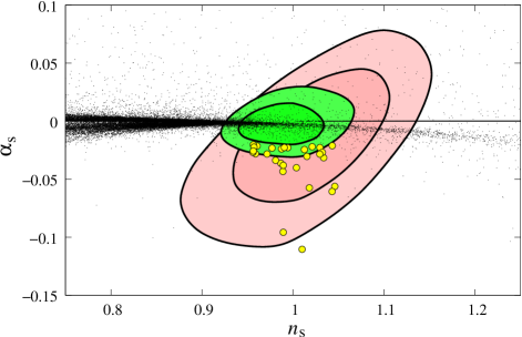
Figure 1: The current constraints (68% and 95% confidence level contours) in the $n_{s}$–$\alpha_{s}$ plane from WMAP+SDSSgal (bigger, red) and WMAP+SDSSlya (smaller, green) data (Seljak et al., 2005; Slosar et al., 2004; Tegmark et al., 2004; Verde et al., 2003). The constrained region clearly allows the value of the spectral scalar index $n_{s}$ to be around $1$ and the running $\alpha_{s}$ of the scalar spectral index to be significantly non-zero for either combination of the experiments.

But it is possible that $|\alpha_{s}|\gg(n_{s}-1)^{2}$ and $\alpha_{s}<0$, which means that the main part in the running of the spectral index (15) is determined not by the first term $-2\epsilon_{1}\epsilon_{2}$, but by the second term $-\epsilon_{2}\epsilon_{3}$. It happens when $|\epsilon_{3}|\gg|\epsilon_{1}|$, and therefore there might be a situation when $|\epsilon_{3}|>1$.

To summarize, if $n_{s}\approx 1$ and $\alpha_{s}$ is a small negative number, at some scale we might have $\epsilon_{1}\ll 1$, $\epsilon_{2}\ll 1$ and $|\epsilon_{3}|>1$. Leach et al. (Leach et al., 2002) define inflation satisfying slow-roll under the condition $|\epsilon_{n}|\ll 1$, for all $n>0$. In our case $\epsilon_{3}>1$, so the question arises as to whether slow-roll in this case is accurate or whether the approximation breaks down and one must also include terms with higher powers in $\epsilon_{3}$. Does it mean that the inflation is not slow-roll and one must use full numerical solutions instead? And does it mean that one must also include the running of the running? These are the main questions we address in this paper. To address them we have developed the numerical code described in appendix A.

How natural is it for inflation with a given number from 50 to 70 e-folds remaining to produce a power spectrum with a changing tilt? In the absence of theoretical guidance on the inflationary space we cannot address this question simply. Authors of Peiris et al. (2003) have produced about 200,000 simulations of the inflationary flow equations for more or less “random” potentials, and calculated the observable parameters ($n_{s}$, $\alpha_{s}$, $r$, $n_{t}$, $\alpha_{t}$) of the resulting power spectra about 40 to 70 e-folds before the end of the inflation for each potential. About 80,000 of them fall into the area plotted on Fig. 1. Only the fifteen marked with larger yellow circles give a significant change in the tilt from red to blue, i.e. $n_{s}\sim 1$, $\alpha_{s}<-0.02$.

Choosing the Hubble parameter to be represented by a Taylor expansion in $\phi$ with uniformly distributed coefficients, as done in Peiris et al. (2003), does not necessarily correspond to the real inflationary priors (Liddle, 2003). We do not address this issue here; instead we want to simply stress that possibility of constructing a potential with a large running in the scalar power spectrum 40-70 e-folds before the end of the inflation exists.

III Quadratic potential

As a test of our code, in this section we investigate how well the slow-roll formulae work in the slow-roll regime for one of the usual potentials that do not predict large running. As an example we will consider a simple quadratic potential, $V=m^{2}\phi^{2}/2$, which is a classic example of chaotic inflation. The second panel from the bottom in Fig. 2 effectively shows the dependence of $z^{\prime\prime}/z$ on the number of the e-folds for inflation with such a potential. The behavior is monotonic and very smooth, which is due to the smoothness of the derivatives of the potential. Since $z^{\prime\prime}/z$ scales as $2a^{2}H^{2}$, we plot the quantity

$$\frac{1}{2a^{2}H^{2}}\frac{z^{\prime\prime}}{z}-1$$ (18)

instead (compare to equation (12)).

The top two panels show the dependence of $\epsilon_{\scriptstyle H}$, $\eta_{\scriptstyle H}$ and $\xi_{\scriptstyle H}$ on the number of e-folds. The only significantly non-zero term is $\epsilon_{\scriptstyle H}$, which gradually grows to $1$ at the end of inflation. The values of $\eta_{\scriptstyle H}$ and $\xi_{\scriptstyle H}$ are typically smaller by roughly $10^{3}$ and $10^{4}$ respectively.

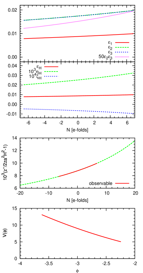
Figure 2: Panels from the bottom to the top: 1. Potential $V=m^{2}\phi^{2}/2$ in the range of $\phi$’s where the inflation occurs around 50 e-folds before the end of inflation. The scale in $V$ is not COBE-normalized on this plot. 2. The dependence of $z^{\prime\prime}/z$ on the number of the e-folds during the inflation. Number of e-folds $N=0$ corresponds to our arbitrarily chosen pivot scale of $k=0.05$/Mpc. 3. Plots of Hubble slow-roll parameters $\epsilon_{\scriptstyle H}$, $\eta_{\scriptstyle H}$, $\xi_{\scriptstyle H}$. The value of $\epsilon_{\scriptstyle H}$ is non-negligible whereas $\eta_{\scriptstyle H}$ and $\xi_{\scriptstyle H}$ are essentially zeros. 4. Plots of horizon-flow slow-roll parameters $\epsilon_{1}$, $\epsilon_{2}$, $\epsilon_{3}$ and the product of $\epsilon_{2}\epsilon_{3}$ for the same inflationary model. Since in this case $\epsilon_{\scriptstyle H}\gg\eta_{\scriptstyle H},\xi_{\scriptstyle H}$, the value of $\epsilon_{1}$ is essentially $\epsilon_{1}\approx\epsilon_{\scriptstyle H}$ and $\epsilon_{2}\approx\epsilon_{3}\approx 2\epsilon_{\scriptstyle H}$. Nothing unexpected is going on here for this model.

Figure 3 shows the primordial power spectrum produced by the quadratic potential. The second panel from the bottom describes the error produced by the slow-roll approximations. The first order approximation gives less than 0.2% error in the observed range of wavenumbers $k$. The second order approximation works slightly better; the error is just above 0.1%. Both of these numbers are likely to be good enough for the upcoming experiments. This is because the accuracy at large scales is limited by the finite number of modes, while at small scales it is limited by the nonlinear evolution. So, while the overall amplitude could in principle be determined to an accuracy of 0.1% when CMB and lensing information is combined, it is unlikely that such a precision will be achieved separately at two widely separated length scales.

Taking a more careful look at the error plot, one sees that the error curve in the observed area is basically a straight line, meaning that the main source of error is not the imprecise value of $\alpha_{s}$ but the error in $n_{s}$. Let us estimate now how precisely we need to know $n_{s}$ to get an error of, say 0.2%, in the observed range. The imprecision $\delta n_{s}$ in $n_{s}$ will give us the uncertainty

$$\delta n_{s}\frac{1}{2}\ln\frac{k_{\max}}{k_{\min}}=0.002.$$ (19)

Taking the observed range of $k$’s to be from $10^{-3}$ Mpc^-1 to $1$ Mpc^-1, we find that one needs to find $n_{s}$ with the precision of $\delta n_{s}=6\cdot 10^{-4}$.

The same allowed uncertainty $\delta\alpha_{s}$ in $\alpha_{s}$ is estimated from

$$\frac{1}{2}\delta\alpha_{s}\left(\frac{1}{2}\ln\frac{k_{\max}}{k_{\min}}\right)^{2}=0.002.$$ (20)

Therefore $\delta\alpha_{s}=3\cdot 10^{-4}$ is the error which we can make in determining $\alpha_{s}$ in order to get an error in the power spectrum of 0.2% at the edges of the observed range of $k$’s.

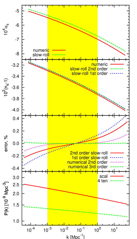
Figure 3: Panels from the bottom to the top: 1. Power spectrum produced by inflation with potential $V=m^{2}\phi^{2}/2$. 2. Errors made by approximating the true scalar power spectrum by (13) with calculating $n_{s}$ and $\alpha_{s}$ from first order slow-roll formulae (16, 17), second order slow-roll formulae (14, 15) and calculating them through numerical derivatives. Numerical third order takes into account third logarithmic derivative of the power spectrum $\beta_{s}$ in parameterization (13). 3. The evolution of $n_{s}-1$ is calculated numerically and by the first and second order slow-roll formulae. 4. The evolution of $\alpha_{s}$ is calculated numerically and by the slow-roll formulae (first and second order slow-roll are the same for $\alpha_{s}$). The error plot clearly shows that the main error comes from the imprecision of $n_{s}-1$, whereas the approximation for the $\alpha_{s}$ works well enough. One can also see that in the case of this potential both first and second order slow-roll formulae for $n_{s}-1$ overestimate the real value of $n_{s}-1$.

The two top panels of Fig. 3 compare the numerically found dependence of $n_{s}$ and $\alpha_{s}$ on $k$ to the one found from the slow-roll approximation with the first order $\alpha_{s}$ and either the first or second order for $n_{s}$. One should compare the discrepancies between these to the values of $\delta n_{s}$ and $\delta\alpha_{s}$. The characteristic value of $n_{s}$ is .964 and the discrepancy between the exact value and the one found from the slow-roll approximation is comparable to $\delta n_{s}$. Running $\alpha_{s}$ takes values around $-6.5\cdot 10^{-4}$. The discrepancy between the exact and the slow-roll values is very small in comparison to $\delta\alpha_{s}$. One can also notice that in this case $|\alpha_{s}|\approx 2\delta\alpha_{s}$. Thus, even if we assigned $\alpha_{s}=0$, we would not get a significant error in the approximation of the primordial power spectrum of the scalar perturbations.

To summarize this section, for standard inflationary potentials, the slow-roll approximation suffices even at first order when compared to the expected accuracy of existing and future experiments. The second order approximation, while improving the accuracy, is not really necessary. The main error of slow-roll when considered in contrast to the numerical solutions is the inaccuracy in the slope $n_{s}$; inaccuracies in higher order expansion terms, such as the running, are less important and can even be ignored.

IV Potential with a bump in the second derivative

We want to construct a potential which will give us a strong running and crossing of the point $n_{s}=1$ in the observable power spectrum. We want to have $n_{s}>1$ at earlier times in inflation, while at later times we want to have $n_{s}<1$. To get the desired result, one can take two different potentials producing such features and smoothly connect them.

One can rewrite slow-roll formulae (14,15) through the potential slow-roll parameters as

$$n_{s}-1 = -6\epsilon_{\scriptstyle V}+2\eta_{\scriptstyle V},$$ (21)

$$\alpha_{s} = 16\epsilon_{\scriptstyle V}\eta_{\scriptstyle V}-24\epsilon_{\scriptstyle V}^{2}-2\xi_{\scriptstyle V}.$$ (22)

Now let us just choose our potential to be

$$V(\phi)=1-0.01\phi-1.20\phi^{2}$$ (23)

for all $\phi>0$. This choice provides about 50 e-folds of inflation after $\phi=0$. Since the local properties of the power spectrum are mostly determined by the local “history” of the slow-roll parameters at the moment of the horizon crossing, we can get a red tilt of the scalar power spectrum $n_{s}\approx 0.80$ in the area where the “history” before point $\phi=0$ is not very important. To get an approximately symmetric shape of the power spectrum we choose $V(\phi)$ to be

$$V(\phi)=1-0.01\phi+1.20\phi^{2}$$ (24)

for all $\phi<0$. In this case for wave modes which cross the horizon far before the moment when the scalar field takes the value of $\phi=0$, the spectral index of the primordial power spectrum has a blue tilt $n_{s}\approx 1.20$. Thus between these two regions the spectral index changes from 1.20 to 0.80. We can unite formulae (23) and (24) into

$$V(\phi)=1-0.01\phi-1.20\phi^{2}\mathop{\mathrm{sign}}\phi.$$ (25)

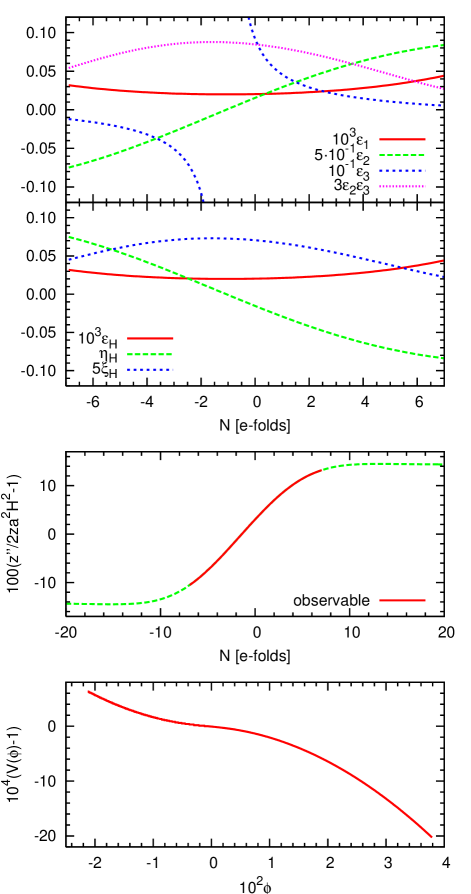
Figure 4: Panels from the bottom to the top: 1. Potential (26). 2. Effectively this plot shows the dependence of $z^{\prime\prime}/z$ on the number of the e-folds during the inflation. 3. Plots of Hubble slow-roll parameters $\epsilon_{\scriptstyle H}$, $\eta_{\scriptstyle H}$, $\xi_{\scriptstyle H}$. Though the potential has a singular behavior, all the flow parameters are smooth. 4. Plots of horizon-flow slow-roll parameters $\epsilon_{1}$, $\epsilon_{2}$, $\epsilon_{3}$ and the product of $\epsilon_{2}\epsilon_{3}$ for the same inflationary model. While everything is fine with $\epsilon_{1}$, $\epsilon_{2}$ and $\epsilon_{2}\epsilon_{3}$, the value of $\epsilon_{3}$ indeed flips over infinity.

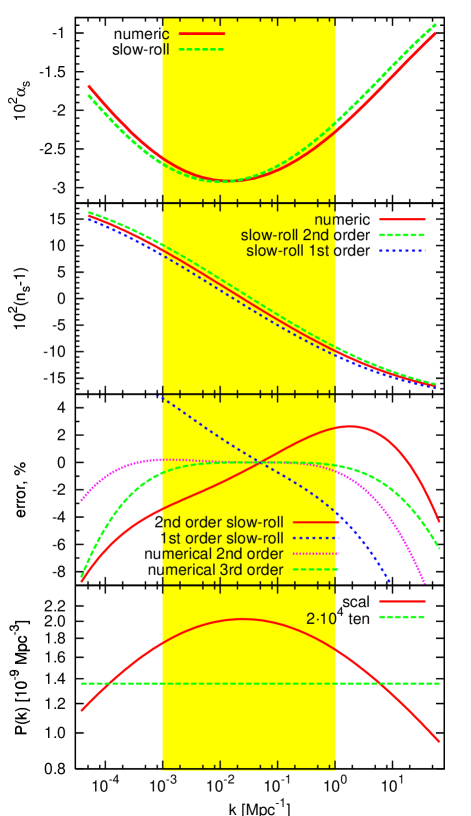
Figure 5: Panels from the bottom to the top: 1. Power spectrum produced by (26). 2. Errors made by approximating the true scalar power spectrum by (13) with calculating $n_{s}$ and $\alpha_{s}$ from first order slow-roll formulae (16, 17), second order slow-roll formulae (14, 15) and calculating them through numerical differentiation. Numerical third order takes into account third logarithmic derivative of the power spectrum $\beta_{s}$ in parameterization (13). 3. The evolution of $n_{s}-1$ is calculated numerically and by the first and second order slow-roll formulae. 4. The evolution of $\alpha_{s}$ is calculated numerically and by the slow-roll formulae (first and second order slow-roll are the same for $\alpha_{s}$). The error plot clearly shows that the main error comes from the imprecision of $n_{s}-1$, whereas the approximation for the $\alpha_{s}$ works well enough. We see that in the case of this potential, first order slow-roll formula for $n_{s}-1$ underestimates the real value, while the second order formula overestimates it.

This potential has continuous first and second derivatives, but has a bump in its third derivative. This makes $\dfrac{1}{z}\dfrac{d^{2}z}{d\tau^{2}}$ in (12) discontinuous around $\phi=0$. According to Starobinskii (1992) this produces oscillations in the power spectrum, which we can indeed see for the potential (25). To avoid the oscillations we smooth out the $\mathop{\mathrm{sign}}\phi$ function, changing it to $\dfrac{2}{\pi}\arctan(200\phi)$. In this case (25) changes to

$$V(\phi)=1-0.01\phi-1.20\phi^{2}\dfrac{2}{\pi}\arctan(200\phi),$$ (26)

which is shown on Fig. 4. We have chosen 200 as the coefficient in front of $\phi$ in the $\arctan$ function so that the produced power spectrum has a nice shape as in Fig. 5.

The two top panels of Fig. 4 show the behavior of the slow-roll parameters $\epsilon_{\scriptstyle H}$, $\eta_{\scriptstyle H}$, $\xi_{\scriptstyle H}$ and $\epsilon_{1}$, $\epsilon_{2}$, $\epsilon_{3}$, $\epsilon_{2}\epsilon_{3}$ correspondingly. While nothing unexpected happens to the behavior of the conventional Hubble slow-roll parameters $\epsilon_{\scriptstyle H}$, $\eta_{\scriptstyle H}$ and $\xi_{\scriptstyle H}$, there appears to be a singularity for the horizon-flow parameter $\epsilon_{3}$. However, notice that the product $\epsilon_{2}\epsilon_{3}$ behaves smoothly and remains small due to the fact that the parameter $\epsilon_{2}$ is changing its sign and therefore crossing through zero. Thus the parameterization of equation (6) introduces a singularity which is not physically present in the model.

Figure 5 shows the power spectrum produced by the model of inflation with the potential (25). The second panel from the bottom shows the errors made by different approximations. We again observe a similar picture for the slow-roll formulae. The main source of error for either the first or second order approximations comes not from the value of $\alpha_{s}$ but from the error in the value of $n_{s}$. From the second panel from the top, we can estimate that the discrepancy is of the order of 0.01 for

$$\delta n_{s}=n_{s}^{\mathrm{exact}}-n_{s}^{\mathrm{approx}}$$ (27)

which gives an error of

$$\delta n_{s}\frac{1}{2}\ln\frac{k_{\max}}{k_{\min}}\approx 4\%$$ (28)

in the produced power spectrum at the edges of the observed range. Both the first and second order slow-roll approximations for $n_{s}$ work somewhat unsatisfactory. The first order slow roll underestimates $n_{s}$ and the second order overestimates it by about the same amount.

On the other hand, if our goal is to focus on running alone regardless of the slope and use just that property to deduce something about the potential, then the slow-roll does very well, since the differences between the slow-roll and numerical value of running are very small even at the lowest order in slow-roll. Extra terms in the expansion (13) further improve the accuracy. Adding running of the running improves the accuracy over the observed range from 1% to 0.2%.

In summary, for potentials that lead to large running, slow-roll does not estimate the slope $n_{s}$ very accurately at either first or second order, while the accuracy of the running $\alpha_{s}$ suffices for the existing and future experiments. If we observe over a wide range of scales then it is useful to add the cubic term. Second order slow-roll does not seem to improve the accuracy.

V Flow Equations Simulations

Kinney Kinney (2002) introduced a formalism based on the so-called flow equations, further discussed in Liddle (2003). The basic idea is that if one fixes the Hubble slow-roll parameters (5) at some point in time for $\epsilon_{\scriptstyle H}$, $\eta_{\scriptstyle H}$ and ${}^{\ell}\xi_{\scriptstyle H}$ up to $\ell=M$ and assumes that all the other Hubble slow-roll parameters are small enough that one can neglect them in one’s calculations (i.e. ${}^{\ell}\xi_{\scriptstyle H}=0$ for all $\ell\geq M+1$) then, without any other assumptions about inflation being slow-roll, one can find the Hubble slow-roll parameters at any other moment of time using the following hierarchy of linear ordinary differential equations:

$$\frac{d\epsilon}{dN} = -2\epsilon(\eta-\epsilon),$$ (29)

$$\frac{d\eta}{dN} = \epsilon\eta-~{}^{2}\xi,$$ (30)

$$\frac{d~{}^{\ell}\xi}{dN} = [\ell\epsilon-(\ell-1)\eta]~{}^{\ell}\xi-~{}^{\ell+1}\xi$$ (31)

for all $\ell=2\dots M$ assuming ${}^{M+1}\xi=0$.

Usually when we set up an inflationary problem, we choose a potential $V(\phi)$ and then reconstruct the form of the Hubble parameter during inflation using the main nonperturbed Hamilton-Jacobi inflationary equation (1), which gives us an attractor solution $H(\phi)$ which in the inflationary class of problems almost does not depend on the initial condition.

By following the method prescribed by Kinney (2002) one avoids solving the main attractor inflationary equation (1), as pointed out by Liddle (2003). Indeed, the assumption ${}^{\ell}\xi_{\scriptstyle H}=0$ for all $\ell\geq M+1$ requires that $H^{(\ell)}(\phi)=0$ for all $\ell\geq M+2$. Consequently, $H(\phi)$ is a polynomial of order $M+1$:

$$H(\phi)=H_{0}(1+A_{1}\phi+A_{2}\phi^{2}+A_{3}\phi^{3}+\dots+A_{M+1}\phi^{M+1}).$$ (32)

In this case the function $H(\phi)$ is an attractor solution of equation (1) with a potential in the form

$$V(\phi)=-\frac{m_{\rm pl}^{4}}{32\pi^{2}}\left([H^{\prime}(\phi)]^{2}-\dfrac{12\pi}{m_{\rm pl}^{2}}H^{2}(\phi)\right)\\ =-\frac{m_{\rm pl}^{4}}{32\pi^{2}}H_{0}^{2}\Biggl{[}\left(A_{1}+\dots+(M+1)A_{M+1}\phi^{M}\right)^{2}\\ -\dfrac{12\pi}{m_{\rm pl}^{2}}\left(1+A_{1}\phi+\dots+A_{M+1}\phi^{M+1}\right)^{2}\Biggr{]}.$$ (33)

Thus the only differential equation one needs to solve in order to match up the number of e-folds and the value of the scalar field $\phi$ is

$$\frac{dN}{d\phi}=\frac{2\sqrt{\pi}}{m_{\rm pl}}\frac{1}{\sqrt{\epsilon(\phi)}}.$$ (34)

Here again $\epsilon(\phi)$ is defined as in the equation (5):

$$\epsilon(\phi)=\frac{m_{\rm pl}^{2}}{4\pi}\left(\frac{H^{\prime}(\phi)}{H(\phi)}\right)^{2}\\ =\frac{m_{\rm pl}^{2}}{4\pi}\left(\frac{A_{1}+2A_{2}\phi+\dots+(M+1)A_{M+1}\phi^{M}}{1+A_{1}\phi+A_{2}\phi^{2}+\dots+A_{M+1}\phi^{M+1}}\right)^{2}.$$ (35)

We do not have to numerically solve the hierarchy of $M$ differential flow equations. Instead we have analytical expressions for $V(\phi)$ and $H(\phi)$.

The late attractor $\epsilon={}^{\ell}\xi=0$ and $\eta=\mathop{\mathrm{const}}$, found by Kinney (2002), corresponds to the situation where the inflation proceeds to the value of the scalar field $\phi$, which is a solution of the equation $\epsilon=0$

$$A_{1}+2A_{2}\phi+\dots+(M+1)A_{M+1}\phi^{M}=0.$$ (36)

At this point if $A_{2}\neq 0$, then $\eta=\mathop{\mathrm{const}}\neq 0$ due to the definition of $\eta$, which does not involve $\epsilon$ at all. All the other ${}^{\ell}\xi=0$ since any of them is a product of the first derivative of the Hubble parameter (which is zero) with some higher order derivatives.

Peiris et al. Peiris et al. (2003) made $M=9$-th order flow equation simulations; about $40,000$ are shown as black dots on Fig. 1. Fifty points fall into the range $|n_{s}-1|<0.05$ and $\alpha_{s}<-0.02$; these are shown in yellow. Among these point we have chosen 13 which fall into the narrow interval $|n_{s}-1|<0.02$, and we have reconstructed the corresponding inflationary potentials for the inflationary models which give such significant running, together with $n_{s}$ extremely close to $1$.

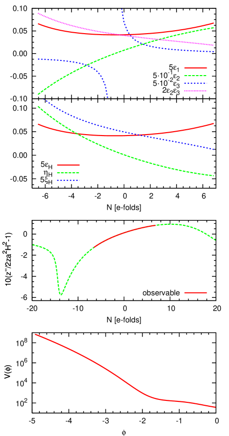
Figure 6: Panels from the bottom to the top: 1. Potential reconstructed from one of the flow equations simulations. 2. Effectively this plot shows the dependence of $z^{\prime\prime}/z$ on the number of the e-folds during the inflation for this potential. 3. Plots of Hubble slow-roll parameters $\epsilon_{\scriptstyle H}$, $\eta_{\scriptstyle H}$, $\xi_{\scriptstyle H}$. All of them are smooth. 4. Plots of horizon-flow slow-roll parameters $\epsilon_{1}$, $\epsilon_{2}$, $\epsilon_{3}$ and the product of $\epsilon_{2}\epsilon_{3}$ for the same inflationary model. While everything is fine with $\epsilon_{1}$, $\epsilon_{2}$ and $\epsilon_{2}\epsilon_{3}$, the value of $\epsilon_{3}$ again flips over infinity.

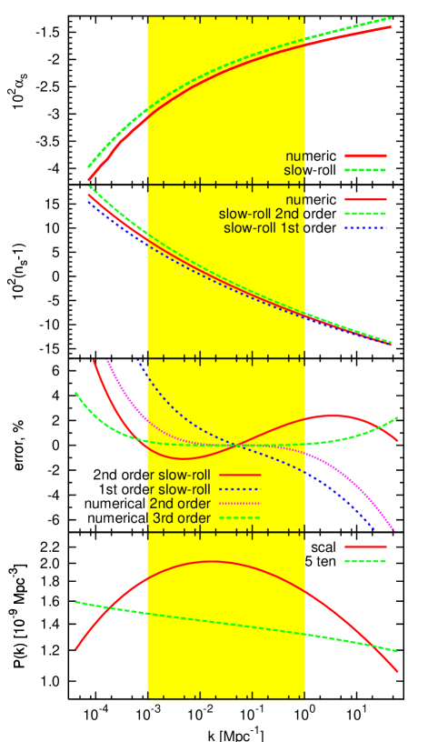
Figure 7: Panels from the bottom to the top: 1. Power spectrum produced by potential on Fig. 6. 2. Errors made by approximating the true scalar power spectrum by (13) with calculating $n_{s}$ and $\alpha_{s}$ from first order slow-roll formulae (16, 17), second order slow-roll formulae (14, 15) and calculating them through numerical differentiation. Numerical third order takes into account third logarithmic derivative of the power spectrum $\beta_{s}$ in parameterization (13). 3. The evolution of $n_{s}-1$ is calculated numerically and by the first and second order slow-roll formulae. 4. The evolution of $\alpha_{s}$ is calculated numerically and by the slow-roll formulae (first and second order slow-roll are the same for $\alpha_{s}$). The error plot clearly shows that the main error comes from the imprecision of $n_{s}-1$, whereas the approximation for the $\alpha_{s}$ works well enough. One can also see that in the case of this potential first order slow-roll formula for $n_{s}-1$ underestimates the real value, while the second order formula overestimates it.

The bottom panel in Fig. 6 shows a potential from such a model with an unusually high value of the running $\alpha_{s}$. We notice that there is a small dip in the potential. Some of the potentials with high $\alpha_{s}$ from the simulations had unrealistically high values of the tensor to the scalar ratio, but all of them had quite similar shapes. The second from the bottom panel of Fig. 6 shows the characteristic behavior of the function $z^{\prime\prime}/z$ which influences the scalar power spectrum as we have seen earlier. The top two panels show the dependence of the slow-roll parameters on the number of e-folds. As in the other case with large running, we find a singularity for the horizon-flow slow-roll parameter $\epsilon_{3}$, while the product $\epsilon_{2}\epsilon_{3}$ behaves smoothly and $\epsilon_{2}$ crosses zero.

The bottom panel in Fig. 7 shows the power spectrum of scalar and tensor perturbations produced by inflation with the potential under consideration. The second from the bottom panel shows the error produced by every one of the approximations for the power spectrum. We again see that both first and second order slow-roll formulae do not give a satisfactory result for $n_{s}$. One of them again overestimates $n_{s}$; the other underestimates it. The error for either of the approximations is about 2–4%.

The error introduced by the approximate formula for the running $\alpha_{s}$ is a bit smaller than the one for $n_{s}$, but it is somewhat larger compared to the quadratic potential we considered in the previous section.

Chen et al. (Chen et al., 2004) perform a similar analysis of slow-roll approximation. Using the flow-equations technique, they found discrepancy of larger than $0.01$ for $n_{s}$ between second and third order slow-roll approximations for some of the models. Based on this fact they conclude that third order slow-roll is better. For the model we considered in this section we have found that the third order slow-roll does not improve the results of the second order approximation. In our calculations both formulas give identical results leading to approximately the same order of error as the first order approximation.

VI Is Truncated Taylor Expansion good?

Recently Abazajian, Kadota and Stewart (Abazajian et al., 2005) have argued that if

$$|\alpha_{s}\ln(k/k_{*})|\gtrsim|n_{s}-1|,$$ (37)

then the traditional truncated Taylor series parameterization is inconsistent, and hence it can lead to incorrect parameter estimations. One can notice that Taylor expansions $P(x)=\sum a_{i}x^{i}$ of functions $x^{2}$ or $\cos x$ around $x=0$ also violates the condition $a_{1}\gtrsim a_{2}x$, but no one argues that these expansions are not valid. Abazajian et al. propose to use the parameterization

$$\ln\mathcal{P}(k)=\ln\mathcal{P}_{0}+\frac{(n_{s}-1)^{2}}{\alpha_{s}}\left[\left(\frac{k}{k_{*}}\right)^{\frac{\alpha_{s}}{n_{s}-1}}-1\right]$$ (38)

instead.

There is one significant disadvantage of this approach. In particular, using this parameterization to describe $\mathcal{P}$ as a function of $k$, one is able to describe only a growing or decreasing function, which can be easily seen from the form of the function. The models we study in this paper produce scalar power spectra which are not purely growing or decreasing (e.g. see Fig. 7).

In the previous section we have considered the potential which produces power spectrum satisfying equation (37). On Fig. 8 we compare the traditional truncated to second and third order Taylor expansion and the parameterization (38). We find that the parameterization (38) gives a significantly larger error than, e.g. the second order Taylor expansion.

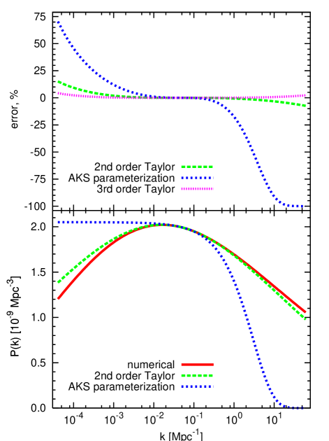
Figure 8: The bottom panel shows the numerically calculated power spectrum of the potential we used in section V and it’s approximations by the second order Taylor expansion and by Abazajian, Kadota and Stewart (AKS) parameterization (38). The top panel shows the error produced by each of the parameterizations. We have also added the error produced by the third order Taylor expansion here. AKS parameterization acceptably describes the true power spectrum in a very narrow range of $k$’s around the pivot point $k=0.05$ Mpc^-1. It does not improve the truncated Taylor expansion over the wider range of $k$’s.

Thus we found that in this particular case though equation (37) holds, truncated Taylor expansion is a good approximation and the AKS approach does not improve it. There might be models for which equation (38) works better than Taylor expansion, but it is definitely not an improvement for a general case and should be used with caution, if at all.

VII Conclusions

In this paper we have explored the accuracy of the slow-roll approximation given the observational constraints on the primordial scalar and tensor power spectra. The current constraints can be roughly described by the tensor to scalar ratio $r<1$, small deviation from the scale invariance of the scalar power spectrum, $|n_{s}-1|<0.05$ and small but possibly nontrivial running, $|\alpha_{s}|<0.03$. These constraints allow for the particular case where $n_{s}\sim 1$ and $|\alpha_{s}|>0.01$, which has previously been argued to not satisfy the slow-roll condition. We have computed exact numerical solutions for the considered potentials and compared them to those obtained from the first and second order slow-roll approximations.

We have found that for the potentials explored here, there is no substantial difference when using first or second order slow-roll formulae for the power spectrum index $n_{s}$. Both of them either work well in the case of small running or have a comparable error in the case of non-negligible running. Adding extra (cubic in $\ln k$) terms in the approximation for the scalar power spectrum extends the accuracy to a larger range of scales, but this accuracy is most likely not necessary for existing and near future experiments. If the values of $n_{s}$ and $\alpha_{s}$ are known with the precision $\delta n_{s}=6\cdot 10^{-4}$ and $\delta\alpha_{s}=3\cdot 10^{-4}$, then the scalar power spectrum will have an error of about 0.2% at the edge of the observable range of wavenumbers $k$’s.

The horizon-flow basis $\epsilon_{n+1}={d\ln|\epsilon_{n}|}/{dN}$ introduces an artificial singularity for inflationary models with negative running and the value of the spectral index crossing 1. Such a divergence in one of the horizon-flow parameters does not indicate that the slow-roll approximation has been badly broken. We find that the slow-roll is still accurate at the 1-2% level and most of the error comes from inaccuracies in the evaluation of the slope itself, and not the running. Thus the first order slow-roll approximation is sufficiently accurate for the current observations. Only if the running turns out to be large, while the slope remains close to scale-invariant, are exact numerical calculations required to achieve sub-percent accuracy. In the appendix we present a short guideline on performing such calculations. One can request the code directly from the author.

*

Appendix A Inflationary Equations

In this appendix we describe the technical details of the code we ran to get the results presented in the main part of the paper. The code is given a potential $V(\phi)$ and some point $\phi_{0}$ which lies in the observable range of wave-modes and, say, corresponds to the moment when wavelengths with $k=0.05$ Mpc^-1 exit the horizon. We want to find the power spectrum produced by inflation with the potential $V(\phi)$. For this purpose we first have to go backwards in time about 50 e-folds and then start the inflation there. This guarantees that the inflationary dynamics are not affected by the choice of the initial condition and we indeed have the attractor solution.

Now we evolve the universe from our “beginning of inflation” to the end of inflation, the moment which is determined by the violation of the inequality $\ddot{a}>0$. This part is described below in the “non-perturbed inflationary equations” section. Usually we require 50 to 70 e-folds between $\phi_{0}$ and the end of inflation.

After we already have the complete background history of the evolution of the universe during the inflationary stage of the expansion, we can start working out the evolution of the perturbations during inflation, as discussed in the second part of the appendix.

A.1 Non-perturbed inflationary equations

The unperturbed dynamics of inflation are described by the equation of motion of the scalar field $\phi$ with potential $V(\phi)$ in the expanding universe with the Hubble parameter $H\equiv\dot{a}/a$

$$\ddot{\phi}+3H\dot{\phi}+V^{\prime}(\phi)=0$$ (39)

and the Friedman equation with only the scalar field component present in the universe

$$H^{2}=\frac{8\pi}{3m_{\rm pl}^{2}}\left[V(\phi)+\frac{1}{2}\dot{\phi}^{2}\right].$$ (40)

The equations (39, 40) are equivalent to the pair of Hamilton-Jacobi equation (1) and

$$\dot{\phi}=-\dfrac{m_{\rm pl}^{2}}{4\pi}H^{\prime}(\phi).$$ (41)

The Hamilton-Jacobi equation connects the Hubble parameter and the value of the potential of the scalar field during the inflation. In the case when we know the behavior of the Hubble parameter it is easy to find the potential. The method of flow equations is entirely based on this fact. In contrast, if we know the shape of the potential and want to reconstruct the behavior of the Hubble parameter, the problem is not as simple. First of all, as for any first order differential equation, we would like to have an initial condition $H_{0}=H(\phi_{0})$. Due to the attractor nature of the equation (1) its solution does not really depend on the initial condition $H_{0}$ (we have found from numerical simulations that one needs about 6 e-folds to forget the history). Thus it does not really matter which initial condition we choose.

Hamilton-Jacobi equation requires that

$$H^{2}(\phi)\geq\frac{8\pi}{3m_{\rm pl}^{2}}V(\phi).$$ (42)

If we are going to use a method such as Runge-Kutta for the integration of the differential equation(1), we might try values of $H$ which would violate the inequality (42).

To avoid this complication, we reparametrize our equation using a new function $\delta(\phi)$ so that

$$H^{2}(\phi)=\frac{8\pi}{3m_{\rm pl}^{2}}V(\phi)\left(1+e^{\delta(\phi)}\right).$$ (43)

Then substituting our new definition into equation (1) we get

$$H^{\prime}(\phi)=-\frac{4\pi\sqrt{2}}{m_{\rm pl}^{2}}\sqrt{V(\phi)}e^{\delta(\phi)/2}.$$ (44)

Combining this with the expression for $H^{\prime}$ obtained from the direct differentiation of $H$ in (43), we get a differential equation for $\delta^{\prime}(\phi)$

$$\delta^{\prime}=-\sqrt{1+e^{-\delta}}\left[\frac{V^{\prime}}{V}\sqrt{1+e^{-\delta}}+\frac{4\sqrt{3\pi}}{m_{\rm pl}}\right].$$ (45)

This equation is much more pleasant to deal with numerically than equation (1), since it does not have a weird boundary for $\delta$, as $H$ did before. One can also check the attractor nature of the equation (45), that it does not remember the prior history. We see now that in the case when the potential is changing slowly $\delta^{\prime}\approx 0$ and we have

$$e^{\delta}=\left[\frac{48\pi}{m_{\rm pl}^{2}\left({V^{\prime}}/V\right)^{2}}-1\right]^{-1}\approx\frac{m_{\rm pl}^{2}}{48\pi}\left(\frac{V^{\prime}}{V}\right)^{2}.$$ (46)

We can use this approximate solution of the equation as the initial condition for our differential equation since it is quite close to the true solution and it will make our numerical solution evolve into the attractor solution faster.

One can check that the expressions for $\epsilon_{\scriptstyle H}$, $\eta_{\scriptstyle H}$ and ${}^{2}\xi_{\scriptstyle H}$ are given by the following formulae

$$\epsilon = \frac{m_{\rm pl}^{2}}{4\pi}\left(\frac{H^{\prime}}{H}\right)^{2}=\frac{3}{1+e^{-\delta}},$$ (47)

$$\eta = \frac{m_{\rm pl}^{2}}{4\pi}\frac{H^{\prime\prime}}{H}$$ (48)

$$= 3+\frac{m_{\rm pl}}{4}\sqrt{\frac{3}{\pi}}\frac{V^{\prime}}{V}\frac{1}{\sqrt{e^{\delta}(1+e^{\delta})}},$$

$${}^{2}\xi = \frac{m_{\rm pl}^{4}}{16\pi^{2}}\frac{H^{\prime}H^{\prime\prime\prime}}{H^{2}}$$ (49)

$$= 3(\epsilon+\eta)-\eta^{2}-\frac{3m_{\rm pl}^{2}}{8\pi}\frac{V^{\prime\prime}}{V}\frac{1}{1+e^{\delta}}.$$

From these expressions we can expect that in general $\epsilon$ and $\eta$ are continuous functions, whereas ${}^{2}\xi$ does not have to be continuous at points where $V^{\prime\prime}$ is not continuous.

The condition for inflation to take place ($\ddot{a}>0$) follows from the derivative of the Friedman equation

$$\frac{\ddot{a}}{a}=\frac{8\pi}{3m_{\rm pl}^{2}}\left[V(\phi)-\dot{\phi}^{2}\right]=H^{2}(\phi)(1-\epsilon),$$ (50)

or

$$\frac{\ddot{a}}{a}=\frac{8\pi}{3m_{\rm pl}^{2}}\left[V(\phi)-\frac{m_{\rm pl}^{4}}{16\pi^{2}}\left(H^{\prime}(\phi)\right)^{2}\right]\\ =\frac{8\pi}{3m_{\rm pl}^{2}}V(\phi)(1-2e^{\delta}).$$ (51)

The first of these two equations implies that the end of inflation happens when the inequality $\epsilon<1$ is violated. The same thing occurs when the inequality $\delta<-\ln 2$ is violated in the second equation. The latter also means that the inflation continues while the kinetic energy of the inflaton is less than half of its potential energy

$$\frac{K}{\Pi}=\frac{\dot{\phi}^{2}/2}{V(\phi)}=e^{\delta(\phi)}<\frac{1}{2}.$$ (52)

Thus we come to a physical definition of our parameter $e^{\delta(\phi)}$ as the ratio of the kinetic energy $\dot{\phi}^{2}/2$ to the potential energy $V(\phi)$.

In the next subsection we will be working with inflationary perturbations and it will not be very convenient for us to work with the value of the scalar field $\phi$ as an independent variable. For this purpose we will use the number of e-folds defined as

$$\tilde{N}=\ln\frac{(aH)}{(aH)_{0}}.$$ (53)

Note that this is the actual number of e-folds and is not the same as $N=\ln(a/a_{0})$. The connection between $\tilde{N}$ and $\phi$ is determined through the derivative

$$\frac{d\tilde{N}}{d\phi}=\frac{2\sqrt{\pi}}{m_{\rm pl}}\frac{1-\epsilon(\phi)}{\sqrt{\epsilon(\phi)}}.$$ (54)

We are almost done describing the background evolution of the universe, except we have not yet chosen the initial value of the scalar field $\phi_{i}$. We only have the value $\phi_{0}$ which corresponds to the moment when the mode $k=0.05$ Mpc^-1 exits the horizon. We want to move backwards in time for about 50 e-folds. Equation (45) has an attractor behavior only when we are moving in the positive direction along the $\phi$-axis. It diverges from the attractor solution in the negative direction. As a useful trick, let us modify equation (1) to the following form

$$[H^{\prime}(\phi)]^{2}=\frac{12\pi}{m_{\rm pl}^{2}}\left[\frac{8\pi}{3m_{\rm pl}^{2}}V(\phi)-H^{2}(\phi)\right].$$ (55)

In this form, when we move backwards in time the value of $H(\phi)$ is bound by the value of $\sqrt{8\pi V/3m_{\rm pl}^{2}}$ from the top and the solution cannot diverge. In addition we temporarily redefine $\delta(\phi)$ to satisfy

$$H^{2}(\phi)=\frac{8\pi}{3m_{\rm pl}^{2}}V(\phi)(1-e^{\delta(\phi)}).$$ (56)

Thus we get an equation analogous to the equation (45)

$$\delta^{\prime}=\sqrt{1-e^{-\delta}}\left[\frac{V^{\prime}}{V}\sqrt{1-e^{-\delta}}+\frac{4\sqrt{3\pi}}{m_{\rm pl}}\right].$$ (57)

Equation (57) does not carry any physical meaning; we just use this equation to go “upwards” to the higher values of the potential, still tracking the general behavior of $V(\phi)$. If we go backwards in time 50 e-folds using (57) and then forward in time 50 e-folds using (45), we will not return to the same point $\phi_{0}$, since the behavior of $\delta(\phi)$ in the equation (57) is determined by the area which is to the right of the current value of $\phi$ and in the equation (45) is determined by the area which is on the left side. Nevertheless, this method gives us a good estimate of what initial value of $\phi_{i}$ we should take.

It is also worth mentioning that this approach is not more  difficult to deal with than the inflationary flow equations (29–31).

A.2 Perturbation equations

A.2.1 Scalar mode

The algorithm for finding the scalar mode primordial power spectrum is described in the main text (see equation (10) and below). Here we will just mention some technical details.

Equation (10) is not very convenient to solve in its current form. First of all we would like to set the independent variable, the conformal time $\tau$, in such a way that $\tau\to-0$ as inflation goes on. In this case we would be able to numerically integrate equation (10) up to as small values of $\tau$ as we want. But in numerical realizations we cannot really choose such an initial value of $\tau_{i}$ that gives us $\tau\to-0$ at the end of the inflation. Suppose that at the end of the inflation we have $\tau\to 1-0$. In this case the numerical error on $\tau$ will be of the order of $10^{-15}$ which is a reasonable machine precision. Hence the limit on corresponding $d\tau$ is of the same order and we can explore the range of changing the scale factor $a$ from $\sim 1$ to $\sim 10^{15}$, i.e. about 35 e-folds. This might be enough, but to be safe we will use a different independent variable, the true number of e-folds $\tilde{N}$ defined by equation (53) which is the same as

$$d\tilde{N}=\frac{d(aH)}{aH}.$$ (58)

Then the mode equation (10) can be rewritten as

$$(1-a)\frac{d^{2}u_{k}}{d\tilde{N}^{2}}+(1+b)\frac{du_{k}}{d\tilde{N}}\\ +\left[\left(\frac{k}{k_{0}}\right)^{2}e^{-2(\tilde{N}-\tilde{N}_{0})}-2(1+c)\right]u_{k}=0,$$ (59)

where coefficient $a$, $b$ and $c$ can be exactly expressed through $\epsilon_{\scriptstyle H}$, $\eta_{\scriptstyle H}$ and ${}^{2}\xi_{\scriptstyle H}$ as

$$a = 2\epsilon-\epsilon^{2},$$ (60)

$$b = -2\epsilon-\epsilon^{2}+2\epsilon\eta,$$ (61)

$$c = \epsilon-\frac{3}{2}\eta+\epsilon^{2}-2\epsilon\eta+\frac{1}{2}\eta^{2}+\frac{1}{2}~{}^{2}\xi.$$ (62)

In equation (59), $k$ is the wavelength of the interest, while $k_{0}$ and $\tilde{N}_{0}$ are constants conveniently chosen for normalization purposes.

Further, equation (10) has a solution

$$u_{k}\propto\frac{1}{\sqrt{2k}}e^{-ik\tau}$$ (63)

at the beginning of the inflation when $\tau\to-\infty$ and $k^{2}\gg\dfrac{1}{z}\dfrac{d^{2}z}{d\tau^{2}}$. We also know the approximate behavior of $u_{k}$ at later times when $\tau\to-0$ and $k^{2}\ll\dfrac{1}{z}\dfrac{d^{2}z}{d\tau^{2}}$:

$$u_{k}\propto z.$$ (64)

Thus it is natural to decompose $u_{k}$ into growing and oscillating parts

$$u_{k}=e^{A+i\phi},$$ (65)

where both functions $A$ and $\phi$ are real functions of conformal time $\tau$ or of the true number of e-folds $\tilde{N}$. Then the equation (59) can be split into 4 ordinary differential equations with 2 new functions $A_{p}$ and $\phi_{p}$ defined as below

$$\frac{dA}{d\tilde{N}} = A_{p},$$ (66)

$$\frac{dA_{p}}{d\tilde{N}} = \frac{-\left.({k^{2}}/{k_{0}^{2}})\right.e^{-2\tilde{N}}+2(1+c)-(1+b)A_{p}}{1-a}$$ (67)

$$-(A_{p}^{2}-\phi_{p}^{2}),$$

$$\frac{d\phi}{d\tilde{N}} = \phi_{p},$$ (68)

$$\frac{d\phi_{p}}{d\tilde{N}} = -\phi_{p}\frac{(1+b)+2(1-a)A_{p}}{1-a}.$$ (69)

This system of differential equations looks a bit more complicated than the single equation (10), but it is actually much easier to solve numerically. Indeed, at earlier times we have $dA/d\tilde{N}\equiv A_{p}=0$. This instaneously gives us the initial condition on $d\phi/d\tilde{N}\equiv\phi_{p}$ from (67)

$$\phi_{p}^{2}=\frac{\left.({k^{2}}/{k_{0}^{2}})\right.e^{-2\tilde{N}}-2(1+c)}{1-a}$$ (70)

as $\tau\to-\infty$, i.e. $\tilde{N}\to-\infty$. To be consistent with the initial condition on

$$u_{k}\propto\dfrac{1}{\sqrt{2k}}e^{-ik\tau}$$

as $\tau\to-\infty$ we also require that

$$A=-\frac{1}{2}\ln k$$

as $\tilde{N}\to-\infty$. As the inflation continues, the terms

$$-\dfrac{k^{2}}{k_{0}^{2}}\dfrac{e^{-2\tilde{N}}}{1-a}$$

and $\phi_{p}^{2}$ will balance each other on the right hand side of the equation (67) until $A_{p}$ is not negligible in comparison to $1$ in equation (69). Thus, around $\tilde{N}=\ln(k/k_{0})$ the oscillating part $\phi_{p}$ will decrease more rapidly than before, finally exponentially dropping to zero. At the same time $A_{p}$, and therefore $A$, start exponentially growing. The final power spectrum is given by

$$\mathcal{P}_{k}=\frac{k^{3}}{2\pi^{2}}\left|\frac{u_{k}}{z}\right|^{2}\propto\frac{k^{3}}{2\pi^{2}}e^{2A_{k}}.$$ (71)

Thus we even do not need information about the phase $\phi$ and we can freely drop equation (68) from our system. Also while being in the stage of inflation where $u_{k}$ has an oscillatory behavior, if one were to use the usual method without our substitution, one would have to find the values of $u_{k}$ for at least 6 points per oscillation period. However with our substitution, we easily pass this area, which does not have any interest for us since we analytically know the behavior of $u_{k}$ here, and therefore move directly to the place where we cannot solve it analytically. By our estimates this technique gives a gain of a factor of 10 in computational time, which is of particular interest if one wants to calculate the power spectrum for e.g. 100 wavemodes.

A.2.2 Tensor mode

The calculation of the tensor mode power spectrum of perturbations is absolutely analogous to the one for scalars, except instead of equation (10) one has to solve

$$\frac{d^{2}u_{k}}{d\tau^{2}}+\left(k^{2}-\frac{1}{a}\frac{d^{2}a}{d\tau^{2}}\right)u_{k}=0$$ (72)

with the same initial condition

$$u_{k}(\tau)\to\dfrac{1}{\sqrt{2k}}e^{-ik\tau}$$

as $\tau\to-\infty$, where $a$ is the usual scale factor of the Friedman universe. One can show that

$$\frac{1}{a}\frac{d^{2}a}{d\tau^{2}}=2a^{2}H^{2}\left(1-\frac{1}{2}\epsilon\right).$$ (73)

Mode equations for the amplitude and the phase of the wave (66-69) of the tensor mode look similar except in the equations (60-62) where we have to change $c$ to $d$ defined as

$$d=-\frac{1}{2}\epsilon.$$ (74)