Constraints on holographic dark energy from type Ia supernova observations

Abstract

In this paper, we use the type Ia supernovae data to constrain the holographic dark energy model proposed by Li. We also apply a cosmic age test to this analysis. We consider in this paper a spatially flat Friedmann-Robertson-Walker Universe with matter component and holographic dark energy component. The fit result shows that the case $c<1$ ($c=0.21$) is favored, which implies that the holographic dark energy behaves as a quintom-type dark energy. Furthermore, we also perform a joint analysis of SNe+CMB+LSS to this model; the result is well improved, and still upholds the quintom dark energy conclusion. The best fit results in our analysis are $c=0.81$, $\Omega_{m}^{0}=0.28$, and $h=0.65$, which lead to the present equation of state of dark energy $w_{0}=-1.03$ and the deceleration/acceleration transition redshift $z_{T}=0.63$. Finally, an expected SNAP simulation using $\Lambda$CDM as a fiducial model is performed on this model, and the result shows that the holographic dark energy model takes on $c<1$ ($c=0.92$) even though the dark energy is indeed a cosmological constant.

I Introduction

The type Ia supernova (SN Ia) [1, 2] observations provide the first evidence for the accelerating expansion of the present Universe. To explain this accelerated expansion, the Universe at present time is viewed as being dominated by an exotic component with large negative pressure referred to as dark energy. A combined analysis of cosmological observations, in particular, of the WMAP (Wilkinson Microwave Anisotropy Probe) experiment [3, 4, 5], indicates that dark energy occupies about 2/3 of the total energy of the Universe, and dark matter about 1/3. The most obvious theoretical candidate of dark energy is the cosmological constant $\Lambda$ [6] which has the equation of state $w=-1$. An alternative proposal is the dynamical dark energy [7, 8] which suggests that the energy form with negative pressure is provided by a scalar field evolving down a proper potential. The feature of this class of models is that the equation of state of dark energy $w$ evolves dynamically during the expansion of the Universe. However, as is well known, there are two difficulties arise from all these scenarios, namely the two dark energy (or cosmological constant) problems — the fine-tuning problem and the “cosmic coincidence” problem. The fine-tuning problem asks why the dark energy density today is so small compared to typical particle scales. The dark energy density is of order $10^{-47}{\rm GeV}^{4}$, which appears to require the introduction of a new mass scale 14 or so orders of magnitude smaller than the electroweak scale. The second difficulty, the cosmic coincidence problem, states “Since the energy densities of dark energy and dark matter scale so differently during the expansion of the Universe, why are they nearly equal today”? To get this coincidence, it appears that their ratio must be set to a specific, infinitesimal value in the very early Universe.

Recently, considerable interest has been stimulated in explaining the observed dark energy by the holographic dark energy model. For an effective field theory in a box of size $L$, with UV cut-off $\Lambda_{c}$ the entropy $S$ scales extensively, $S\sim L^{3}\Lambda_{c}^{3}$. However, the peculiar thermodynamics of black hole [9] has led Bekenstein to postulate that the maximum entropy in a box of volume $L^{3}$ behaves nonextensively, growing only as the area of the box, i.e. there is a so-called Bekenstein entropy bound, $S\leq S_{BH}\equiv\pi M_{p}^{2}L^{2}$. This nonextensive scaling suggests that quantum field theory breaks down in large volume. To reconcile this breakdown with the success of local quantum field theory in describing observed particle phenomenology, Cohen et al. [10] proposed a more restrictive bound – the energy bound. They pointed out that in quantum field theory a short distance (UV) cut-off is related to a long distance (IR) cut-off due to the limit set by forming a black hole. In the other words, if the quantum zero-point energy density $\rho_{X}$ is relevant to a UV cut-off, the total energy of the whole system with size $L$ should not exceed the mass of a black hole of the same size, thus we have $L^{3}\rho_{X}\leq LM_{p}^{2}$, this means that the maximum entropy is in order of $S_{BH}^{3/4}$. When we take the whole Universe into account, the vacuum energy related to this holographic principle [11] is viewed as dark energy, usually dubbed holographic dark energy. The largest IR cut-off $L$ is chosen by saturating the inequality so that we get the holographic dark energy density

$$\rho_{X}=3c^{2}M_{p}^{2}L^{-2}~{},$$ (1)

where $c$ is a numerical constant, and $M_{p}\equiv 1/\sqrt{8\pi G}$ is the reduced Planck mass. If we take $L$ as the size of the current Universe, for instance the Hubble scale $H^{-1}$, then the dark energy density will be close to the observed data. However, Hsu [12] pointed out that this yields a wrong equation of state for dark energy. Li [13] subsequently proposed that the IR cut-off $L$ should be taken as the size of the future event horizon

$$R_{h}(a)=a\int_{t}^{\infty}{dt^{\prime}\over a(t^{\prime})}=a\int_{a}^{\infty}{da^{\prime}\over Ha^{\prime 2}}~{},$$ (2)

then the problem can be solved nicely and the holographic dark energy model can thus be constructed successfully. Some speculations on the deep reasons of the holographic dark energy were considered by several authors [14]; further studies on this model see also [15, 16, 17, 18, 19, 20, 21, 22, 23]. In addition, it is necessary to discuss about the choice $L=H^{-1}$. Even though this choice was argued to be unsuitable due to that it may lead to the holographic dark energy tracks the matter density, this does not mean that the formalism $M_{p}^{2}H^{2}$ cannot be made compatible with the observation. There are other contexts in quantum field theory where one can have a dark energy behaving as $M_{p}^{2}H^{2}$ without introducing the holographic principle. For instance, Refs.[24] nicely introduce the $M_{p}^{2}H^{2}$ law from general arguments in quantum field theory. Actually, the first time where this law was introduced in quantum field theory was in the context of the renormalization group models of the cosmological constant; see e.g. [25]. Otherwise, within the holographic model framework, the choice $L=H^{-1}$ can also be favored, if one introduce some interaction between dark energy and dark matter [23]. However, in this paper we restrict our attention to the holographic dark energy model proposed by Li [13].

In this paper, we will see what constraints to the holographic dark energy model are set by present and future SNe Ia observations. Recently, some constraints from SNe Ia on related model where obtained in Refs.[16, 17]. In this paper, we extend the analysis carried out in Ref.[16]. The work presented here differs from [16] (and [17]) in the following aspects: (a) We not only constrain the model by means of the SNe Ia observations, but also test the fit results by using the age of the Universe; (b) When performing the analysis of the SNe data, we also test the sensitivity to the present Hubble parameter $H_{0}$ in the fit; (c) For improving the fit result, we combine the current SNe Ia data with the cosmic microwave background (CMB) data and the large-scale structure (LSS) data to analyze the model; (d) We also investigate the predicted constraints on the model from future SNe Ia observations.

II The holographic dark energy model

The holographic dark energy scenario may provide simultaneously natural solutions to both dark energy problems as demonstrated in Ref.[13]. In what follows we will review this model briefly and then constrain it by the type Ia supernova observations. In addition, we will also apply a joint analysis of SNe+CMB+LSS data to this model. Consider now a spatially flat FRW (Friedmann-Robertson-Walker) Universe with matter component $\rho_{m}$ (including both baryon matter and cold dark matter) and holographic dark energy component $\rho_{X}$, the Friedmann equation reads

$$3M_{p}^{2}H^{2}=\rho_{m}+\rho_{X}~{},$$ (3)

or equivalently,

$${H^{2}\over H_{0}^{2}}=\Omega_{m}^{0}a^{-3}+\Omega_{X}{H^{2}\over H_{0}^{2}}~{}.$$ (4)

Note that we always assume spatial flatness throughout this paper as motivated by inflation. Combining the definition of the holographic dark energy (1) and the definition of the future event horizon (2), we derive

$$\int_{a}^{\infty}{d\ln a^{\prime}\over Ha^{\prime}}={c\over Ha\sqrt{\Omega_{X}}}~{}.$$ (5)

We notice that the Friedmann equation implies

$${1\over Ha}=\sqrt{a(1-\Omega_{X})}{1\over H_{0}\sqrt{\Omega_{m}^{0}}}~{}.$$ (6)

Substituting (6) into (5), one obtains the following equation

$$\int_{x}^{\infty}e^{x^{\prime}/2}\sqrt{1-\Omega_{X}}dx^{\prime}=ce^{x/2}\sqrt{{1\over\Omega_{X}}-1}~{},$$ (7)

where $x=\ln a$. Then taking derivative with respect to $x$ in both sides of the above relation, we get easily the dynamics satisfied by the dark energy, i.e. the differential equation about the fractional density of dark energy,

$$\Omega_{X}^{\prime}=\Omega_{X}(1-\Omega_{X})(1+{2\over c}\sqrt{\Omega_{X}})~{},$$ (8)

where the prime denotes the derivative with respect to $x$. This equation describes the behavior of the holographic dark energy completely, and it can be solved exactly [13, 16],

$$\ln\Omega_{X}-{c\over 2+c}\ln(1-\sqrt{\Omega_{X}})+{c\over 2-c}\ln(1+\sqrt{\Omega_{X}})-{8\over 4-c^{2}}\ln(c+2\sqrt{\Omega_{X}})=-\ln(1+z)+y_{0}~{},$$ (9)

where $y_{0}$ can be determined through (9) by replacing $\Omega_{X}$ with $\Omega_{X}^{0}$ as $z=0$. From the energy conservation equation of the dark energy, the equation of state of the dark energy can be expressed as

$$w=-1-{1\over 3}{d\ln\rho_{X}\over d\ln a}~{}.$$ (10)

Then making use of the formula $\rho_{X}={\Omega_{X}\over 1-\Omega_{X}}\rho_{m}^{0}a^{-3}$ and the differential equation of $\Omega_{X}$ (8), the equation of state for the holographic dark energy can be given [13, 16, 17]

$$w=-{1\over 3}(1+{2\over c}\sqrt{\Omega_{X}})~{}.$$ (11)

We can also give the deceleration parameter $q=-\ddot{a}/aH^{2}$, in terms of $\Omega_{X}$,

$$q={1\over 2}-{1\over 2}\Omega_{X}-{1\over c}\Omega_{X}^{3/2}~{}.$$ (12)

It can be seen clearly that the equation of state of the holographic dark energy evolves dynamically and satisfies $-(1+2/c)/3\leq w\leq-1/3$ due to $0\leq\Omega_{X}\leq 1$. In this sense, this model should be attributed to the class of dynamical dark energy models even though without quintessence scalar field. The parameter $c$ plays a significant role in this model. If one takes $c=1$, the behavior of the holographic dark energy will be more and more like a cosmological constant with the expansion of the Universe, and the ultimate fate of the Universe will be entering the de Sitter phase in the far future. As is shown in Ref.[13], if one puts the parameter $\Omega_{X}^{0}=0.73$ into (11), then a definite prediction of this model, $w_{0}=-0.903$, will be given. On the other hand, if $c<1$, the holographic dark energy will behave like a quintom-type dark energy proposed recently in Ref.[26], the amazing feature of which is that the equation of state of dark energy component $w$ crosses the phantom divide line, $-1$, i.e. it is larger than $-1$ in the past while less then $-1$ near today. The recent fits to current SNe Ia data with parametrization of the equation of state of dark energy find that the quintom-type dark energy is mildly favored [27, 28, 29]. Usually the quintom dark energy model is realized in terms of double scalar fields, one is a normal scalar field and the other is a phantom-type scalar field [30, 31]. However, the holographic dark energy in the case $c<1$ provides us with a more natural realization for the quintom picture. While, if $c>1$, the equation of state of dark energy will be always larger than $-1$ such that the Universe avoids entering the de Sitter phase and the Big Rip phase. Hence, we see explicitly, the determination of the value of $c$ is a key point to the feature of the holographic dark energy as well as the ultimate fate of the Universe.

FIG. 1.: An illustrative example for the holographic dark energy model. The evolutions of the deceleration parameter $q$ and the equation of state of dark energy $w$. In this case, we take $\Omega_{m}^{0}=0.27$.

As an illustrative example, we plot in Fig.1 the evolutions of the deceleration parameter $q$ and the equation of state of dark energy $w$ in cases of $c=1.2,~{}1.0,~{}0.8$ and 0.6, respectively. It is easy to see that the equation of state of dark energy crosses $-1$ as $c<1$, which is in accordance with the plots of the model-independent analysis in Ref.[27]. It should be pointed out that the variable cosmological constant model can also give rise to a quintom behavior, i.e. the effective equation of state produced by this model can also cross $-1$ [32].

In the forthcoming sections, we will see what constraints to the model described above are set by present and future SNe Ia observations. In the fitting, we use the recent new high red-shift supernova observations from the HST/GOODS program and previous supernova data, and furthermore we test the fit results by means of the cosmic age data. We find that if we marginalize the nuisance parameter $h$, the fit of the SNe observation provides $0.09\lesssim c\lesssim 0.62~{}(1\sigma)$; this means the holographic dark energy behaves as a quintom. Further, we find that the allowed range of model parameters depends on $h$ evidently, for instance, we obtain (in $1\sigma$) $0.21\lesssim c\lesssim 1.17$ for $h=0.64$, $0.10\lesssim c\lesssim 0.43$ for $h=0.66$, and $0.03\lesssim c\lesssim 0.07$ for $h=0.71$. The allowed regions of model parameters become evidently smaller for larger values of $h$. The fit values of the matter density $\Omega_{m}^{0}$ in this model are apparently larger than the fit value appears in the $\Lambda$CDM (WMAP result). Now that the SNe data analysis evidently depends on the value of $h$, an important thing we should do is to find some observational quantities which do not depend on $h$ to be useful complements of the SNe data set to probe the property of holographic dark energy. Such quantities can be found in CMB and LSS (${\cal R}$ and $A$, respectively, see section IV). A combined analysis of SNe+CMB+LSS shows that the confidence region evidently shrinks, and the value of $c$ is changed considerably, namely in $1\sigma$, $0.65\lesssim c\lesssim 1.04$. We will discuss the cosmological consequences come from the fits, and compare the case of the joint analysis with the case of the SNe only in detail. Interestingly, an expected SNAP simulation using $\Lambda$CDM as a fiducial model shows that the holographic dark energy model will also favor $c<1$ even though the Universe is indeed dominated by a cosmological constant.

III The current type Ia supernova constraints

We now perform the best fit analysis on our holographic dark energy model with data of the type Ia supernova observations. The luminosity distance of a light source is defined in such a way as to generalize to an expanding and curved space the inverse-square law of brightness valid in a static Euclidean space,

$$d_{L}=\left({{\cal L}\over 4\pi{\cal F}}\right)^{1/2}=H_{0}^{-1}(1+z)\int_{0}^{z}{dz^{\prime}\over E(z^{\prime})}~{},$$ (13)

where ${\cal L}$ is the absolute luminosity which is a known value for the standard candle SNe Ia, $\cal F$ is the measured flux, $H_{0}^{-1}$ (here we use the natural unit, namely the speed of light is defined to be 1) represents the Hubble distance with value $H_{0}^{-1}=2997.9h^{-1}$ Mpc, and $E(z)=H(z)/H_{0}$ can be obtained from (4), expressed as

$$E(z)=\left({\Omega_{m}^{0}(1+z)^{3}\over 1-\Omega_{X}}\right)^{1/2}~{},$$ (14)

note that the dynamical behavior of $\Omega_{X}$ is determined by (8). The observations directly measure the apparent magnitude $m$ of a supernova and its red-shift $z$. The apparent magnitude $m$ is related to the luminosity distance $d_{L}$ of the supernova through

$$m(z)=M+5\log_{10}(d_{L}(z)/{\rm Mpc})+25~{},$$ (15)

where $M$ is the absolute magnitude which is believed to be constant for all type Ia supernovae. The numerical parameter $c$ of the model, the density parameter $\Omega_{m}^{0}$ and the nuisance parameter $h$ can be determined by minimizing

$$\chi^{2}=\sum_{i}{[\mu_{\rm obs}(z_{i})-\mu_{\rm th}(z_{i})]^{2}\over\sigma_{i}^{2}}~{},$$ (16)

where the extinction-corrected distance moduli $\mu(z)$ is defined as $\mu(z)=m(z)-M$, and $\sigma_{i}$ is the total uncertainty in the observation. The likelihood ${\cal L}\propto e^{-\chi^{2}/2}$ if the measurement errors are Gaussian. In our analysis, we take the 157 gold data points listed in Riess et al. [33] which includes recent new 14 high redshift SNe (gold) data from the HST/GOODS program. The results of our analysis for the holographic dark energy model are displayed in Fig.2. In this figure we marginalize over the nuisance parameter $h$ and show $68\%$, $95\%$ and $99\%$ confidence level contours, in the $(c,\Omega_{m}^{0})$-plane. The best fit values for the model parameters are: $h=0.66$, $\Omega_{m}^{0}=0.47^{+0.06}_{-0.15}$, and $c=0.21^{+0.41}_{-0.12}$ with $\chi_{\rm min}^{2}=173.44$ (similar results see also [16]). We see clearly that the fit values of this model are evidently different from those of $\Lambda$CDM, i.e. the value of $h$ is slightly smaller and $\Omega_{m}^{0}$ evidently larger (The WMAP results for $\Lambda$CDM model are [4, 34]: $h=0.71^{+0.04}_{-0.03}$ and $\Omega_{m}^{0}=0.27\pm 0.04$). We notice in this figure that the current SNe Ia data do not strongly constrain the parameters $\Omega_{m}^{0}$ and $c$ (in $2\sigma$), in particular $c$, in the considered ranges. Other observations may impose further constraints. For instance, the CMB and LSS data can provide us with useful complements to the SNe data for constraining cosmological models. But, first, we will apply a cosmic age test to the SNe analysis.

FIG. 2.: Confidence contours of $68\%,~{}95\%$ and $99\%$ in the $(c,\Omega_{m}^{0})$-plane for the case of marginalizing $h$. The point in the figure, with the coordinate $(0.21,0.47)$, represents the best fit value, with $\chi^{2}_{\rm min}=173.44$. Constraints from the age of the Universe give $0.95<H_{0}t_{0}<1.05$ (at the $1\sigma$ confidence level), the dashed lines represent these two limits.

Recent analyses of the age of old stars [35] indicate that the expansion time is in the range $11{\rm Gyr}\lesssim t_{0}\lesssim 17{\rm Gyr}$ at $95\%$ confidence, with a central value $t_{0}\simeq 13{\rm Gyr}$. Following Krauss and Chaboyer [35] these numbers add 0.8 Gyr to the star ages, under the assumption that star formation commenced no earlier than $z=6$. A naive addition in quadrature to the uncertainty in $H_{0}$ indicates that the dimensionless age parameter is in the range $0.72\lesssim H_{0}t_{0}\lesssim 1.17$ at $95\%$ confidence, with a central value $H_{0}t_{0}\simeq 0.89$. More recent, Richer et al. [36] and Hansen et al. [37] found an age of $12.7\pm 0.7$ Gyr at $95\%$ confidence using the white dwarf cooling sequence method. For a full review of cosmic age see Ref. [4]. All in all, it seems reasonable to view $\sim 12$ Gyr to be a low limit of the cosmic age [38]. Now let us examine the age computation of the holographic dark energy model. The age of the Universe can be written as

$$t_{0}=H_{0}^{-1}\int_{0}^{\infty}{dz\over(1+z)E(z)}~{},$$ (17)

where $H_{0}^{-1}$ represents the Hubble time with value $H_{0}^{-1}=9.778h^{-1}$ Gyr. Using the best fit values, the holographic dark energy model gives the cosmic age $t_{0}=13.3$ Gyr. This value is consistent with the above observational analyses. Furthermore, we impose a more rigorous test on it. The latest value of cosmic age appears in the Review of Particle Physics (PDG) [34] is given by a combined analysis of various observations [4], $t_{0}=13.7\pm 0.2$. Using the data from Ref.[34], we can get the dimensionless age parameter range $0.96\lesssim H_{0}t_{0}\lesssim 1.05$ at $68\%$ confidence, with a central value $H_{0}t_{0}\simeq 0.99$. We also display the contours $H_{0}t_{0}=0.96$ and $H_{0}t_{0}=1.05$ ($1\sigma$) in Fig.2. It can be seen explicitly that the $1\sigma$ fit result of the SNe Ia data is almost excluded by this age test.

FIG. 3.: Confidence contours of $68\%,~{}95\%$ and $99\%$ in the $(c,\Omega_{m}^{0})$-plane for the case of $h=0.64$. The best fit values for the parameters are: $\Omega_{m}^{0}=0.41^{+0.12}_{-0.18}$ and $c=0.46^{+0.71}_{-0.25}$, with $\chi_{\rm min}^{2}=175.90$. Dashed lines represent the contours of cosmic age with $t_{0}=12,~{}13,~{}14,~{}15,~{}16$ and 18 Gyr.

FIG. 4.: Confidence contours of $68\%,~{}95\%$ and $99\%$ in the $(c,\Omega_{m}^{0})$-plane for the case of $h=0.66$. The best fit values for the parameters are: $\Omega_{m}^{0}=0.47^{+0.07}_{-0.11}$ and $c=0.21^{+0.22}_{-0.11}$, with $\chi_{\rm min}^{2}=173.44$. Dashed lines represent the contours of cosmic age with $t_{0}=12,~{}13,~{}14,~{}15$ and 16 Gyr.

FIG. 5.: Confidence contours of $68\%,~{}95\%$ and $99\%$ in the $(c,\Omega_{m}^{0})$-plane for the case of $h=0.71$. The best fit values for the parameters are: $\Omega_{m}^{0}=0.49\pm 0.03$ and $c=0.05\pm 0.02$, with $\chi_{\rm min}^{2}=175.90$. Dashed lines represent the contours of cosmic age with $t_{0}=11,~{}12,~{}13,~{}14$ and 16 Gyr.

Next, we will probe the sensitivity to the present Hubble parameter $H_{0}$ in the analysis of the SNe data. We check that, keeping the parameter $h$ fixed, how well the SNe and the cosmic age will constrain the holographic dark energy model. We fix $h=0.64,~{}0.66$ and 0.71, respectively, and show the fit results in Figs.3-5. From these figures, we notice that with the increase of the parameter $h$, $c$ decreases evidently and the confidence contours in the $(c,\Omega_{m}^{0})$-plane shrink sharply. These figures clearly show that the SNe analysis is dependent on the parameter $h$ highly. Hence, finding out observational quantities which do not depend on $H_{0}$ to jointly constrain the holographic dark energy model becomes very important and senseful. We also display age contours in these figures, but the age constraints are rather weak. The fits of SNe data indicate that the current SNe Ia data tend to support a holographic dark energy with $c<1$, in other words, a quintom-type holographic dark energy. However, the authors of Ref.[17] tried to show another possibility. They re-examined the holographic dark energy model by considering the spatial curvature, and found that the holographic dark energy will not behave as phantom if the Universe is closed. However, the spatial flatness is a definitive prediction of the inflationary cosmology, and has been confirmed precisely by the WMAP. Thus we use the spatial flatness prior throughout this paper.

IV combined analysis with CMB and LSS

The above analyses show that the supernovae data alone seem not sufficient to constrain the holographic dark energy model strictly. First, the confidence region of $c-\Omega_{m}^{0}$ plane is rather large, especially for the parameter $c$. Moreover, the best fit value of $\Omega_{m}^{0}$ is evidently larger. Second, it is very hard to understand the fit value of parameter $c$, 0.21, it seems odd because it leads to an unreasonable present equation of state, $w_{0}=-2.64$, the absolute value is too large. Third, even though the predicted cosmic age $t_{0}=13.3$ Gyr is larger than the reasonable low limit of the cosmic age estimated by old stars, a more rigorous analysis implies that the fit result of the SNe Ia data is contradictive to the present data of cosmic age (dimensionless age parameter $H_{0}t_{0}$). Furthermore, our analysis shows that the fit of the SNe Ia data is very sensitive to the parameter $H_{0}$. Hence, it is very important to find other observational quantities irrelevant to $H_{0}$ as complement to SNe Ia data. Fortunately, such suitable data can be found in the probes of CMB and LSS.

In what follows we will perform a combined analysis of SNe Ia, CMB, and LSS on the constraints of the holographic dark energy model. We use a $\chi^{2}$ statistic

$$\chi^{2}=\chi_{\rm SN}^{2}+\chi_{\rm CMB}^{2}+\chi_{\rm LSS}^{2}~{},$$ (18)

where $\chi_{\rm SN}^{2}$ is given by equation (16) for SNe Ia statistics, $\chi_{\rm CMB}^{2}$ and $\chi_{\rm LSS}^{2}$ are contributions from CMB and LSS data, respectively. For the CMB, we use only the measurement of the CMB shift parameter [39],

$${\cal R}=\sqrt{\Omega_{m}^{0}}\int_{0}^{z_{\rm dec}}{dz\over E(z)}~{},$$ (19)

where $z_{\rm dec}=1089$ [3]. Note that this quantity is irrelevant to the parameter $H_{0}$ such that provides robust constraint on the dark energy model. The results from CMB data correspond to ${\cal R}_{0}=1.716\pm 0.062$ (given by WMAP, CBI, ACBAR) [4, 40]. We include the CMB data in our analysis by adding $\chi_{\rm CMB}^{2}=[({\cal R}-{\cal R}_{0})/\sigma_{\cal R}]^{2}$ (see [41]), where ${\cal R}$ is computed by the holographic dark energy model using equation (19). The only large scale structure information we use is the parameter $A$ measured by SDSS [42], defined by

$$A=\sqrt{\Omega_{m}^{0}}E(z_{1})^{-1/3}\left[{1\over z_{1}}\int_{0}^{z_{1}}{dz\over E(z)}\right]^{2/3}~{},$$ (20)

where $z_{1}=0.35$. Also, we find that this quantity is independent of $H_{0}$ either, thus can provide another robust constraint on the model. The SDSS gives the measurement data [42] $A_{0}=0.469\pm 0.017$. We also include the LSS constraints in our analysis by adding $\chi_{\rm LSS}^{2}=[(A-A_{0})/\sigma_{A}]^{2}$ (see [43]), where $A$ is computed by the holographic dark energy model using equation (20).

Note that we have chosen to use only the most conservative and robust information, ${\cal R}$ and $A$, from CMB and LSS observations. These measurements we use do not depend on the Hubble parameter $H_{0}$. Furthermore, by limiting the amount of information that we use from CMB and LSS observations to complement the SNe Ia data, we minimize the effect of the systematics inherent in the CMB and LSS data on our results. Figure 6 shows our main results, the contours of $1\sigma$, $2\sigma$, and $3\sigma$ confidence levels in the $c-\Omega_{m}^{0}$ plane. The best fit values for the model parameters are: $h=0.65$, $\Omega_{m}^{0}=0.28\pm 0.03$, and $c=0.81^{+0.23}_{-0.16}$, with $\chi_{\rm min}^{2}=176.67$. We see clearly that a great progress has been made when we perform a joint analysis of SNe Ia, CMB, and LSS data. Note that the best fit value of c is also less than 1, while in $1\sigma$ range it can slightly larger than 1. Now the fit value of $\Omega_{m}^{0}$ is roughly as the same as that of the $\Lambda$CDM model (WMAP result), but $h$ is still slightly smaller. It should be pointed out that a slightly lower value of $h$ is, however, in agreement with the observations of [44] which can accommodate lower values of $h\sim 0.6$. We also see from the figure that the fit result of the joint analysis is consistent with the dimensionless age range $0.96\lesssim H_{0}t_{0}\lesssim 1.05$.

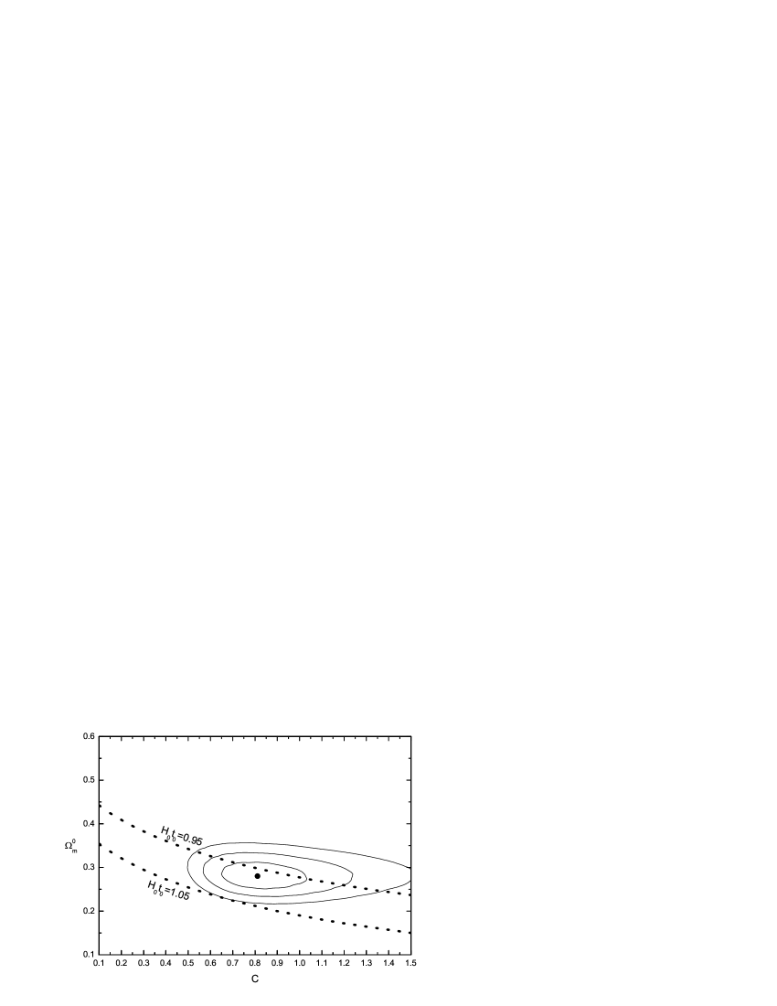
FIG. 6.: Results for analysis of SNe+CMB+LSS data, $1\sigma$, $2\sigma$, $3\sigma$ confidence levels in the $c-\Omega_{m}^{0}$ space, marginalizing over $h$. The best fit values are: $h=0.65$, $\Omega_{m}^{0}=0.28$, and $c=0.81$, with $\chi_{\rm min}^{2}=176.67$. Cosmic age test, the dimensionless age parameter range $0.96\lesssim H_{0}t_{0}\lesssim 1.05$, also shown.

We now compare the fit results of the SNe analysis and the joint analysis of SNe, CMB, and LSS, and discuss the different cosmological consequences. Let us first look at the likelihood distributions of the parameter $c$ in the two fits. In Fig.7 we plot the 1-dimensional likelihood function for $c$, marginalizing over the other parameters. The big difference can lead to rather different conclusions for some important cosmological parameters, such as today’s equation-of-state parameter of dark energy, today’s deceleration parameter, etc. For the best fit results of the two fits, we plot the evolution behaviors of the deceleration parameter $q$ and the equation-of-state parameter of dark energy $w$ in Fig.8. For the SNe+CMB+LSS joint analysis, from the figure, we see that the deceleration parameter $q$ has a value of $q_{0}=-0.61$ at present. The transition from deceleration to acceleration ($q(z_{T})=0$) occurs at a redshift of $z_{T}=0.63$. The equation-of-state parameter $w$ is slightly smaller than $-1$ at present, $w_{0}=-1.03$. For comparison, we list these values for the alone analysis of SNe data: $q_{0}=-1.60$, $z_{T}=0.27$, and $w_{0}=-2.64$. Therefore, obviously, the results of the combined fit seem more reasonable. From a joint analysis of SNe+CMB+LSS data, one may obtain within the framework of the holographic dark energy model a fairly good idea of when the Universe began to accelerate and how fast the present acceleration is. By contraries, the cosmological consequences given by the alone analysis of the SNe data seem unreasonable. Comparing our plots in Fig.8 with the model-independent plots in Ref.[27] (which also use data from [33]), we find that the holographic plot for $c=0.81$ case is in good agreement with those model-independent plots for the redshift range $z=0-2$, while the $c=0.21$ case dose not accord. Moreover, it should be mentioned again that these results demonstrate that the best fit to SNe+CMB+LSS observations also favors a quintom-type holographic dark energy.

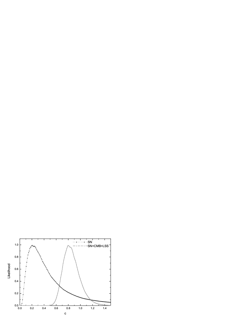
FIG. 7.: Likelihood distributions of parameter $c$ in the fits of SNe only and SNe+CMB+LSS.

FIG. 8.: Deceleration parameter $q$ and equation of state of dark energy $w$, versus red-shift $z$, from two fits, SNe only and SNe+CMB+LSS. Solid lines correspond to the joint analysis of SNe+CMB+LSS, with the parameters $c=0.81$, $\Omega_{m}^{0}=0.28$, and $h=0.65$. Dashed lines correspond to the alone analysis of SNe, with the parameters $c=0.21$, $\Omega_{m}^{0}=0.47$, and $h=0.66$.

V Expected SNAP analysis

Finally we consider how well the proposed Supernova/Acceleration Probe (SNAP), may constrain the parameters $c$ and $\Omega_{m}^{0}$. The SNAP mission is expected to observe about 2000 type Ia SNe each year, over a period of three years, according to the SNAP specifications.To find the expected precision of the SNAP, one must assume a fiducial model, and then simulate the experiment assuming it as a reference model. We will use SNAP specifications to construct mock SNe catalogues [45]. Following previous investigations [46], we assume, in our Monte Carlo simulations, that a total of 2000 supernovae (roughly one year of SNAP observations) will be observed with the following redshift distribution. We consider, 1920 SNe Ia, distributed in 24 bins, from $z=0$ to $z=1.2$. From redshift $z=1.2$ to $z=1.5$, we assume that 60 SNe Ia will be observed and we divide them in 6 bins. From $z=1.5$ to $z=1.7$ we consider 4 bins with 5 SNe Ia in each bin. All the supernovae are assumed to be uniformly distributed with $\Delta z=0.05$. To fully determine the $\chi^{2}$ functions, the error estimates for SNAP must be defined. Following [45], we assume that the systematic errors for the apparent magnitude, $m$, are given by

$$\sigma_{sys}={0.02\over 1.5}z~{}~{},$$ (21)

which are measured in magnitudes such that at $z=1.5$ the systematic error is $0.02$ mag, while the statistical errors for $m$ are estimated to be $\sigma_{sta}=0.15$ mag. We add both kinds of errors quadratically

$$\sigma_{mag}(z_{i})=\sqrt{\sigma^{2}_{sys}(z_{i})+{\sigma^{2}_{sta}\over n_{i}}}~{}~{},$$ (22)

where $n_{i}$ is the number of supernovae in the $i^{\prime}th$ redshift bin with width $\Delta z\approx 0.05$. Now let us assume a spatial flat $\Lambda$CDM model as a fiducial model, and analyze the holographic dark energy model fit. We aim to show if the Universe is indeed described by the $\Lambda$CDM model, how well the the fitting of a holographic dark energy model to be.

FIG. 9.: Predicted confidence contours of $68\%,~{}95\%$ and $99\%$ in the $(c,\Omega_{m}^{0})$-plane for the SNAP mission are shown. We consider a fiducial model with $\Omega_{m}^{0}=0.27$ and $h=0.71$. The best fit values for the parameters are: $\Omega_{m}^{0}=0.23$ and $c=0.92$.

In Fig.9 we display the results of our simulation assuming a $\Lambda$CDM model as fiducial model with $\Omega_{m}^{0}=0.27$ and $h=0.71$. In the fit, we marginalize over the nuisance parameter $h$. The best fit values for the model parameters are: $\Omega_{m}^{0}=0.23$ and $c=0.92$. From this figure it is clear that SNAP mission is able to place rigorous constraints on the holographic dark energy model. On the other hand, we notice with interest that, even though the dark energy in the Universe is exactly described by a cosmological constant $\Lambda$, the precision type Ia supernova observations will still support a quintom-type holographic dark energy.

VI Concluding remarks

In this paper, we investigated constraints on the holographic dark energy model from current and future SN Ia observations. We considered a spatially flat FRW Universe with matter component and holographic dark energy component. For the holographic dark energy model, the numerical constant $c$ plays a very important role in determining the evolutionary behavior of the space-time as well as the ultimate fate of the Universe. In a holographic dark energy dominated Universe, the case of $c=1$ corresponds to an asymptotic de Sitter Universe; The choice of $c<1$ will lead to dark energy behaving as quintom, and in this case, the Gibbons-Hawking entropy will eventually decrease as the event horizon shrink such that violates the second law of thermodynamics; While the case of $c>1$ does not violate the second law of thermodynamics, in this situation, the evolution of the corresponding space-time avoids entering de Sitter phase and Big Rip phase. Though the choice of $c=1$ is favored theoretically, other possibilities can not be ruled out from the viewpoint of phenomenology, and only experiments and observations are capable of determining which choice is realistic. We derived model parameter ranges from the analysis of the present available SNe Ia data, and then imposed a rigorous test using the new data of age of the Universe on the derived parameter region. However, only the supernova analysis seems not sufficient to be able to precisely determine the value of $c$. For improving the result of the analysis, we perform a joint analysis of SNe, CMB, and LSS data to the holographic dark energy model.

The results of the SNe analysis show that the holographic dark energy model behaves as quintom in $1\sigma$ confidence level, consistent with the current SNe Ia data. However, when we perform a rigorous age test on this analysis result using the latest PDG data, the $1\sigma$ allowed range is almost ruled out. Moreover, in this case, the confidence regions in the parameter-plane are rather large. We also probe the sensitivity to the present Hubble parameter $H_{0}$ in this analysis. We do this by fixing the parameter $h$, and find the allowed regions of the parameters shrink sharply as $h$ increases. Hence, a combined analysis of SNe data with other observational data becomes important. A joint analysis of SNe+CMB+LSS produces more reasonable results: $c=0.81$, $\Omega_{m}^{0}=0.28$, and $h=0.65$, leading to the present equation of state of dark energy is $w_{0}=-1.03$, and the epoch at which the Universe began to accelerate is $z_{T}=0.63$. The confidence regions in this analysis become more compact. On the whole, the analysis indicates that the case of $c<1$ is consistent with the present SNe Ia data.

We are also interested in the constraints on the holographic dark energy model from a fictitious future supernova experiment. An expected SNAP fit, by using the $\Lambda$CDM model as fiducial model to generate mock observational data, shows that the case $c<1$ ($c=0.92$) also favored. Obviously, a large number of supernovae at high redshifts, as well as better knowledge of the values of $H_{0}$ and $\Omega_{m}^{0}$ are therefore required to draw firm conclusions about the property of the holographic dark energy. We expect that a more sophisticated combined analysis of various observations will be capable of determining the value of $c$ exactly and thus revealing the property of the holographic dark energy.

- [1] A. G. Riess et al., Astron. J. 116 (1998) 1009 astro-ph/9805201.
- [2] S. Perlmutter et al., Astrophys. J. 517 (1999) 565 astro-ph/9812133.
- [3] C. L. Bennett et al., Astrophys. J. Suppl. 148 (2003) 1 astro-ph/0302207.
- [4] D. N. Spergel et al., Astrophys. J. Suppl. 148 (2003) 175 astro-ph/0302209.
- [5] H. V. Peiris et al., Astrophys. J. Suppl. 148 (2003) 213 astro-ph/0302225.
- [6] S. Weinberg, Rev. Mod. Phys. 61 (1989) 1; S. M. Carroll, Living Rev. Rel. 4 (2001) 1 astro-ph/0004075; P. J. E. Peebles and B. Ratra, Rev. Mod. Phys. 75 (2003) 559 astro-ph/0207347; T. Padmanabhan, Phys. Rept. 380 (2003) 235 hep-th/0212290.
- [7] C. Wetterich, Nucl. Phys. B 302 (1988) 668; P. J. E. Peebles and B. Ratra, Astrophys. J. 325 (1988) L17; B. Ratra and P. J. E. Peebles, Phys. Rev. D 37 (1988) 3406; J. A. Frieman, C. T. Hill, A. Stebbins and I. Waga, Phys. Rev. Lett. 75 (1995) 2077 astro-ph/9505060; M. S. Turner and M. White, Phys. Rev. D 56 (1997) R4439 astro-ph/9701138; R. R. Caldwell, R. Dave and P. J. Steinhardt, Phys. Rev. Lett. 80 (1998) 1582 astro-ph/9708069; A. R. Liddle and R. J. Scherrer, Phys. Rev. D 59 (1999) 023509 astro-ph/9809272; I. Zlatev, L. Wang and P. J. Steinhardt, Phys. Rev. Lett. 82 (1999) 896 astro-ph/9807002; P. J. Steinhardt, L. Wang and I. Zlatev, Phys. Rev. D 59 (1999) 123504 astro-ph/9812313; D. F. Torres, Phys. Rev. D 66 (2002) 043522 astro-ph/0204504.
- [8] L. Amendola, Phys. Rev. D 62 (2000) 043511 astro-ph/9908023; L. Amendola, D. Tocchini-Valentini, Phys. Rev. D 64 (2001) 043509 astro-ph/0011243; L. Amendola, D. Tocchini-Valentini, Phys. Rev. D 66 (2002) 043528 astro-ph/0111535; L. Amendola, Mon. Not. Roy. Astron. Soc. 342 (2003) 221 astro-ph/0209494; M. Pietroni, Phys. Rev. D 67 (2003) 103523 hep-ph/0203085; D. Comelli, M. Pietroni, and A. Riotto, Phys. Lett. B 571 (2003) 115 hep-ph/0302080; U. Franca, and R. Rosenfeld, Phys. Rev. D 69 (2004) 063517 astro-ph/0308149; X. Zhang, astro-ph/0503072; X. Zhang, Phys. Lett. B 611 (2005) 1 astro-ph/0503075.
- [9] J. D. Bekenstein, Phys. Rev. D 7 (1973) 2333; J. D. Bekenstein, Phys. Rev. D 9 (1974) 3292; J. D. Bekenstein, Phys. Rev. D 23 (1981) 287; J. D. Bekenstein, Phys. Rev. D 49 (1994) 1912; S. W. Hawking, Commun. Math. Phys. 43 (1975) 199; S. W. Hawking, Phys. Rev. D 13 (1976) 191.
- [10] A. G. Cohen, D. B. Kaplan and A. E. Nelson, Phys. Rev. Lett. 82 (1999) 4971 hep-th/9803132.
- [11] G. ’t Hooft, gr-qc/9310026; L. Susskind, J. Math. Phys. 36 (1995) 6377 hep-th/9409089.
- [12] S. D. H. Hsu, Phys. Lett. B 594 (2004) 13 hep-th/0403052.
- [13] M. Li, Phys. Lett. B 603 (2004) 1 hep-th/0403127.
- [14] K. Ke and M. Li, Phys. Lett. B 606 (2005) 173 hep-th/0407056; S. Hsu and A. Zee, hep-th/0406142;Y. Gong, Phys. Rev. D 70 (2004) 064029 hep-th/0404030; Y. S. Myung, Phys. Lett. B 610 (2005) 18; Y. S. Myung, hep-th/0501023; H. Kim, H. W. Lee and Y. S. Myung, hep-th/0501118; Y. S. Myung, hep-th/0502128.
- [15] Q. G. Huang and M. Li, JCAP 0408 (2004) 013 astro-ph/0404229; Q. G. Huang and M. Li, JCAP 0503 (2005) 001 hep-th/0410095.
- [16] Q. G. Huang and Y. Gong, JCAP 0408 (2004) 006 astro-ph/0403590.
- [17] Y. Gong, B. Wang and Y. Z. Zhang, hep-th/0412218.
- [18] H. C. Kao, W. L. Lee and F. L. Lin, Phys. Rev. D 71 (2005) 123518 astro-ph/0501487.
- [19] K. Enqvist and M. S. Sloth, Phys. Rev. Lett. 93 (2004) 221302 hep-th/0406019. K. Enqvist, S. Hannestad and M. S. Sloth, JCAP 0502 (2005) 004 astro-ph/0409275.
- [20] J. Shen, B. Wang, E. Abdalla and R. K. Su, hep-th/0412227.
- [21] E. Elizalde, S. Nojiri, S. D. Odintsov and P. Wang, hep-th/0502082.
- [22] X. Zhang, astro-ph/0504586.
- [23] D. Pavon, and W. Zimdahl, gr-qc/0505020; B. Wang, Y. Gong, and E. Abdalla, hep-th/0506069.
- [24] T. Padmanabhan, hep-th/0406060; T. Padmanabhan, Curr. Sci. 88 (2005) 1057 astro-ph/0411044.
- [25] I. L. Shapiro, J. Sola, C. Espana-Bonet, and P. Ruiz-Lapuente, Phys. Lett. B 574 (2003) 149 astro-ph/0303306; C. Espana-Bonet, P. Ruiz-Lapuente, I. L. Shapiro, and J. Sola, JCAP 0402 (2004) 006 hep-ph/0311171; I. L. Shapiro, J. Sola, and H. Stefancic, JCAP 0501 (2005) 012 hep-ph/0410095.
- [26] B. Feng, X. Wang and X. Zhang, Phys. Lett. B 607 (2005) 35 astro-ph/0404224.
- [27] U. Alam, V. Sahni, and A. A. Starobinsky, JCAP 0406 (2004) 008 astro-ph/0403687.
- [28] D. Huterer and A. Cooray, Phys. Rev. D 71 (2005) 023506 astro-ph/0404062.
- [29] See also, e.g. S. Nesseris and L. Perivolaropoulos, Phys. Rev. D 70 (2004) 043531 astro-ph/0401556; R. A. Daly and S. G. Djorgovski, Astrophys. J. 612 (2004) 652 astro-ph/0403664; S. W. Allen, R. W. Schmidt, H. Ebeling, A. C. Fabian, and L. van Speybroeck, Mon. Not. Roy. Astron. Soc. 353 (2004) 457 astro-ph/0405340; T. R. Choudhury and T. Padmanabhan, Astron. Astrophys. 429 (2005) 807 astro-ph/0311622; H. K. Jassal, J. S. Bagla and T. Padmanabhan, Mon. Not. Roy. Astron. Soc. Lett. 356 (2005) L11 astro-ph/0404378; S. Hannestad and E. Mortsell, JCAP 0409 (2004) 001 astro-ph/0407259; P. S. Corasaniti, M. Kunz, D. Parkinson, E. J. Copeland and B. A. Bassett, Phys. Rev. D 70 (2004) 083006 astro-ph/0406608; D. A. Dicus and W. W. Repko, Phys. Rev. D 70 (2004) 083527 astro-ph/0407094; B. A. Bassett, P. S. Corasaniti, and M. Kunz, Astrophys. J. 617 (2004) L1 astro-ph/0407364.
- [30] For relevant studies see e.g. S. Nojiri and S. D. Odintsov, Phys. Lett. B 562 (2003) 147 hep-th/0303117; S. Nojiri and S. D. Odintsov, Phys. Lett. B 599 (2004) 137 astro-ph/0403622; E. Elizalde, S. Nojiri and S. D. Odintsov, Phys. Rev. D 70 (2004) 043539 hep-th/0405034; Y. H. Wei and Y. Tian, Class. Quant. Grav. 21 (2004) 5347 gr-qc/0405038; C. Csaki and N. Kaloper, astro-ph/0409596; Y. Wang, J. M. Kratochvil, A. Linde, M. Shmakova, JCAP 0412 (2004) 006 astro-ph/0409264; V. K. Onemli and R. P. Woodard, Class. Quant. Grav. 19 (2002) 4607 gr-qc/0204065; T. Brunier, V. K. Onemli, R. P. Woodard, Class. Quant. Grav. 22 (2005) 59-84 gr-qc/0408080; B. McInnes, JHEP 0410 (2004) 018 hep-th/0407189; G. Allemandi, A. Borowiec and M. Francaviglia, Phys. Rev. D 70 (2004) 103503 hep-th/0407090; E. Babichev, V. Dokuchaev and Y Eroshenko, Class. Quant. Grav. 22 (2005) 143 astro-ph/0407190; A. Vikman, Phys. Rev. D 71 (2005) 023515 astro-ph/0407107; Z. H. Zhu and J. S. Alcaniz Astrophys. J. 620 (2005) 7 astro-ph/0404201; V. K. Onemli and R. P. Woodard, gr-qc/0406098; S. D. H. Hsu, A. Jenkins and M. B. Wise, Phys. Lett. B 597 (2004) 270 astro-ph/0406043; G. Chen and B. Ratra, Astrophys. J. 612 (2004) L1 astro-ph/0405636; T. Padmanabhan, astro-ph/0411044; B. Feng, M. Li, Y. Piao and X. Zhang, astro-ph/0407432; J. Xia, B. Feng and X. Zhang, astro-ph/0411501; S. Nojiri, S. D. Odintsov and S. Tsujikawa, hep-th/0501025; H. Wei, R.-G. Cai and D.-F. Zeng, hep-th/0501160; M. Li, B. Feng, and X. Zhang, hep-ph/0503268.
- [31] Z. Guo, Y. Piao, X. Zhang and Y. Zhang, Phys. Lett. B 608 (2005) 177 astro-ph/0410654; X. Zhang, H. Li, Y. Piao and X. Zhang, astro-ph/0501652.
- [32] J. Sola, and H. Stefancic, astro-ph/0505133.
- [33] A. G. Riess et al., Astrophys. J. 607 (2004) 665 astro-ph/0402512.
- [34] Particle Data Group, S. Eidelman et al., Review of Particle Physics, Phys. Lett. B 592 (2004) 92.
- [35] E. Carretta et al. Astrophys. J. 533 (2000) 215; L. M. Krauss and B. Chaboyer, astro-ph/0111597; B. Chaboyer and L. M. Krauss, Astrophys. J. Lett. 567 (2002) L45 astro-ph/0201443.
- [36] H. B. Richer et al. Astrophys. J. 574 (2002) L151.
- [37] B. M. S. Hansen et al. Astrophys. J. 574 (2002) L155.
- [38] B. Feng, X. Wang and X. Zhang, Phys. Lett. B 607 (2005) 35 astro-ph/0404224.
- [39] J. R. Bond, G. Efstathiou, and M. Tegmark, Mon. Not. Roy. Astron. Soc. 291 (1997) L33 astro-ph/9702100; A. Melchiorri, L. Mersini, C. J. Odman, and M. Trodden, Phys. Rev. D 68 (2003) 043509 astro-ph/0211522; C. J. Odman, A. Melchiorri, M. P. Hobson, and A. N. Lasenby, Phys. Rev. D 67 (2003) 083511 astro-ph/0207286.
- [40] CBI Collaboration, T. J. Pearson et al., Astrophys. J. 591 (2003) 556 astro-ph/0205388; ACBAR Collaboration, C. L. Kuo et al., Astrophys. J. 600 (2004) 32 astro-ph/0212289.
- [41] Y. Wang, and P. Mukherjee, Astrophys. J. 606 (2004) 654 astro-ph/0312192; Y. Wang, and M. Tegmark, Phys. Rev. Lett. 92 (2004) 241302 astro-ph/0403292.
- [42] D. J. Eisenstein et al., astro-ph/0501171.
- [43] Y. Gong, and Y.-Z. Zhang, astro-ph/0502262.
- [44] A. Saha et al., Astrophys. J. 486 (1997) 1; G. A. Tammann, A. Sandage, and B. Reindl, Astron. Astrophys. 404 (2003) 423 astro-ph/0303378; P. D. Allen, and T. Shanks, Mon. Not. Roy. Astron. Soc. 347 (2004) 1011A astro-ph/0102447; W. L. Freedman et al., Astrophys. J. 553 (2001) 47 astro-ph/0012376; E. S. Battistelli et al., Astrophys. J. 598 (2003) L75 astro-ph/0303587; E. D. Reese et al., Astrophys. J. 581 (2002) 53 astro-ph/0205350; B. S. Mason, S. T. Myers, and A. C. S. Readhead, Astrophys. J. 555 (2001) L11 astro-ph/0101169.
- [45] See, e.g. J. Weller, A. Albrecht, Phys. Rev. D 65 (2002) 103512 astro-ph/0106079; M. Makler, S. Oliveira and I. Waga, Phys.Lett. B 555 (2003) 1 astro-ph/0209486; U. Alam, V. Sahni, T. Saini, A. A. Starobinsky, Mon. Not. Roy. Astron. Soc. 344 (2003) 1057 astro-ph/0303009; O. Bertolami, A. A. Sen, S. Sen and P. T. Silva, Mon. Not. Roy. Astron. Soc. 353 (2004) 329 astro-ph/0402387.
- [46] I. Maor, R. Brustein and P. J. Steinhardt, Phys. Rev. Lett. 86 (2001) 6 astro-ph/0007297; J. Weller and A. Albrecht, Phys. Rev. Lett. 86 (2001) 1939 astro-ph/0008314; J. Weller and A. Albrecht, Phys. Rev. D 65 (2002) 103512 astro-ph/0106079; S. Podariu, P. Nugent and B. Ratra, Astrophys. J. 553 (2001) 39 astro-ph/0008281; M. Goliath, R. Amanullah, P. Astier and R. Pain, Astronomy & Astrophysics 380 (2001) 6 astro-ph/0104009; S. C. C. Ng and D. L. Wiltshire, Phys. Rev. D 64 (2001) 123519 astro-ph/0107142; Y. Wang and G. Lovelace, Astrophys. J. 562 (2001) L115 astro-ph/0109233; E. M. Minty, A. F. Heavens and M. R. S. Hawkins, Mon. Not. Roy. Astron. Soc. 330 (2002) 378 astro-ph/0104221 ; A. G. Kim, E. V. Linder, R. Miquel and N. Mostek, Mon. Not. Roy. Astron. Soc. 347 (2004) 909-920 astro-ph/0304509.