Deriving stellar properties from photometry: maximizing information content and minimizing biases

Abstract

I study the importance of the accurate calibration of photometric systems in order to produce meaningful comparisons between the observed colors + magnitudes and model SEDs. Possible sources of errors are discussed and two examples are analyzed. I show that well-calibrated Tycho-2 photometry is stable and precise enough for such comparisons. On the contrary, the available calibrations for Johnson $UBV$ photometry yield relative large systematic errors, which has prompted me to develop a new, more precise calibration. The advantages of multicolor photometry over the standard single-color + magnitude diagrams for the derivation of physical properties of stars (elimination of degeneracies, inclusion of multiple parameters, avoidance of linearizing approximations, possibility of a more precise treatment of errors) are discussed through the use of CHORIZOS, a code developed specifically for this purpose.

Space Telescope Science Institute, 3700 San Martin Drive, Baltimore, MD 21218, U.S.A.

Space Telescope Division, European Space Agency, ESTEC, Noordwijk, Netherlands

1. A brief introduction to synthetic photometry

 The most common way of studying the properties of stellar populations is by comparing measured single-color + magnitude diagrams (SCMDs) with the synthetic magnitudes derived from spectral energy distributions (SEDs) by means of a synthetic photometry code. The formula used to compute the magnitude for a photon-counting detector is:

$$m_{P}=-2.5\log_{10}\left(\frac{\int P(\lambda)f_{\lambda}(\lambda)\lambda\,d\lambda}{\int P(\lambda)f_{\lambda{\rm,ref}}(\lambda)\lambda\,d\lambda}\right)+{\rm ZP}_{P}$$ (1)

and the equivalent formula for an energy-integrating detector is:

$$m_{P}^{\prime}=-2.5\log_{10}\left(\frac{\int P(\lambda)f_{\lambda}(\lambda)\,d\lambda}{\int P(\lambda)f_{\lambda{\rm,ref}}(\lambda)\,d\lambda}\right)+{\rm ZP}^{\prime}_{P}.$$ (2)

The quantities in those formulae are:

• $f_{\lambda}(\lambda)$ is the SED of the object.

• $f_{\lambda{\rm,ref}}(\lambda)$ is the SED of the reference spectrum. The most common choices are Vega, a constant in $f_{\lambda}$, and a constant in $f_{\nu}$ (see Fig. 1).

• $P(\lambda)$ is the total-system sensitivity curve.

• ZP_P (or ZP${}^{\prime}_{P}$) is the zero point for filter $P$.

Figure 1.: Reference spectra for magnitude systems: the Vega spectrum of Bohlin & Gilliland (2004), the constant $f_{\lambda}$ spectrum for the ST system, and the constant $f_{\nu}$ spectrum for the AB system. The latter two are normalized to have the same flux (in photons s^-1 cm^-2 Å^-1) at $\lambda=5493$ Å (dotted line). The non-normalized photon-counting sensitivity curves for the Tycho-2 $B_{T}$ and $V_{T}$ filters are also plotted.

A magnitude system for a filter $P$ is defined by giving both $f_{\lambda{\rm,ref}}(\lambda)$ and ZP_P. Common choices are:

• The VEGAMAG system uses Vega as a reference spectrum and has ZP_P = 0 by definition (STScI 1998).

• The STMAG system also has ZP_P = 0 and as a reference spectrum uses a constant in $f_{\lambda}$ normalized in such a way as to have the same flux as Vega at the pivot wavelength of the Johnson $V$ filter, 5493 Å. We obtain a value of $f_{\lambda}=3.582\cdot 10^{-9}$ erg s^-1 cm^-2 Å^-1 from the Vega spectrum of Bohlin & Gilliland (2004).

• The ABMAG system also has ZP_P = 0 and as a reference spectrum uses a constant in $f_{\nu}$ normalized in such a way as to have the same flux as Vega at the pivot wavelength of the Johnson $V$ filter, 5493 Å. We obtain a value of $f_{\nu}=3.605\cdot 10^{-20}$ erg s^-1 cm^-2 Hz^-1 from the Vega spectrum of Bohlin & Gilliland (2004).

• The Johnson-Cousins system uses Vega as a reference spectrum and has values of $ZP_{P}$ for $P=U,B,V\ldots$ that NEED TO BE MEASURED.

There are some possible error sources that can yield biases when using synthetic photometry. The first one is using the wrong equation (1 or 2). Since Eq. 1 gives more weight to longer wavelengths, it generates brighter magnitudes for red objects than for blue ones compared to Eq. 2. This can be quantified e.g. by computing $\Delta m=(m_{P,1}-m_{P,1}^{\prime})-(m_{P,2}-m_{P,2}^{\prime})$ for a red (1) and a blue (2) SED (Table 1), since that quantity gives the maximum systematic error introduced in the analysis of a CMD. If one wants to convert between energy-integrating and photon-counting magnitudes it is useful to define a sensitivity curve $P^{\prime}(\lambda)=P(\lambda)/\lambda$. Then, it is easy to show that $m_{P^{\prime}}=m_{P}^{\prime}$ if ZP${}_{P^{\prime}}$ = ZP${}^{\prime}_{P}$.

	Johnson-Cousins					Strömgren
Filter	$U$	$B$	$V$	$R$	$I$	$u$	$v$	$b$	$y$
$\Delta m$	0.049	0.053	0.037	0.054	0.020	0.019	0.003	0.001	0.024

Table 1.: $\Delta m$ for Johnson-Cousins and Strömgren filters using as red and blue spectra solar-metallicity main-sequence Kurucz models with $T_{\rm eff}$ of 3 500 K and 50 000 K, respectively.

A second possible source of errors is an incorrect $f_{\lambda{\rm,ref}}(\lambda)$. For the case of Vega, the most precise spectrum is the one obtained by Bohlin & Gilliland (2004) using a combination of HST/STIS CCD spectroscopy and Kurucz models. The absolute flux calibration has an accuracy of 4% in the FUV and 2% in the optical (Bohlin 2000) but, given that the photometric repeatability of STIS is 0.2-0.4% (Bohlin et al. 2001), the relative flux calibration for colors derived from STIS spectra is expected to be better than 2% in the optical.

Two other possible sources of error are an incorrect knowledge of $P(\lambda)$ and of ZP_P. In the next two sections we analyze the cases of the Tycho-2 $B_{T}V_{T}$ and Johnson $UBV$ filter sets.

2. Calibration of Tycho-2 $B_{T}V_{T}$ photometry

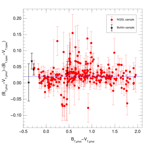
Figure 2.: Comparison between photometric and spectrophotometric Tycho-2 $B_{T}-V_{T}$ colors as a function of photometric $B_{T}-V_{T}$ for the two samples. The error bars represent the photometric uncertainties and the horizontal line marks the proposed ZP${}_{B_{T}-V_{T}}$.

 The Hipparcos mission (ESA 1997) observed the full sky and yielded the Tycho catalog, which is reasonably complete down to $V=11.5$. The original Tycho catalog was consequently reprocessed by Høg et al. (2000b) to produce the Tycho-2 catalog, which contains 2.5 million stars and is currently the most complete and accurate all-sky photometric survey in the optical. The Tycho-2 catalog contains photometry in two optical bands, $B_{T}$ and $V_{T}$, whose sensitivities were analyzed by Bessell (2000) and use Vega as the reference spectrum. The careful processing of Tycho-2 photometry was described by Høg et al. (2000a), including the different tests used to check for possible systematic errors.

I have recently (Maíz Apellániz 2005) tested the sensitivity curves of the Tycho-2 photometry and calculated the values of ZP${}_{B_{T}}$, ZP${}_{V_{T}}$, and ZP${}_{B_{T}-V_{T}}$ using the spectra obtained with STIS for the Next Generation Spectral Library (or NGSL, http://lifshitz.ucdavis.edu/~mgregg/gregg/ngsl/ngsl.html and Gregg et al. 2004) and the spectrophotometric standards of Bohlin et al. (2001). The results for $B_{T}-V_{T}$ are shown in Figs. 2 and 3. No general trend is observed as a function of color in Fig. 2 and the data are symmetrically distributed around a central value, which I take to be ZP${}_{B_{T}-V_{T}}$. I measured ZP${}_{B_{T}-V_{T}}$ by calculating the weighted mean using $1/\sigma^{2}_{B_{T}-V_{T}}$ as weights and found it to be 0.020$\pm$0.001 magnitudes. The histograms for the $B_{T}-V_{T}$ data, both in absolute and relative (corrected for ZP${}_{B_{T}-V_{T}}$ and dividing each point by its photometric uncertainty) terms, appear in Fig. 3. The second histogram has a median of $1.2\cdot 10^{-5}$ and a standard deviation of 1.04 and the distribution is very well approximated by a normalized Gaussian. All of the above implies that an accurate cross-calibration of colors vs. relative fluxes between Tycho-2 photometry and HST spectrophotometry is possible in principle without having to invoke e.g. modifications in the Tycho filter sensitivities or the STIS calibration. Furthermore, given that the normalized histogram has a standard deviation only slightly larger than 1.0, the largest source of deviations from the expected value originates in the photometry, not in the spectrophotometry. Since the mean photometric $\sigma_{B_{T}-V_{T}}$ = 0.025 magnitudes, the accuracy of the spectrophotometrically-derived Tycho-2 colors must be better than 1%, which agrees with the published value for the STIS photometric repeatability Bohlin et al. (2001). A similar analysis for the individual magnitudes $B_{T}$ and $V_{T}$ yields ZP${}_{B_{T}}$ = 0.078$\pm$0.009 magnitudes and ZP${}_{V_{T}}$ = 0.058$\pm$0.009.

Figure 3.: Histograms for the comparison between photometric and spectrophotometric $B_{T}-V_{T}$ colors for the NGSL sample. (left) Regular histogram. (right) Histogram for the data shifted by the proposed ZP${}_{B_{T}-V_{T}}$ and normalized by the individual uncertainties. A Gaussian distribution with $\mu=0$ and $\sigma=1$ is overplotted for comparison.

These results imply that the Tycho-2 photometry has well-characterized sensitivity curves and that the zero points are accurate and stable, both in absolute and relative terms. Therefore, it should be possible to produce accurate comparisons between Tycho-2 photometry and synthetic photometry generated from SED models.

3. Calibration of Johnson $UBV$ photometry

 The Johnson (1966) $UBV$ system is the most commonly used photometric system in the optical range. It was originally defined using photomultipliers but it was later adapted for CCDs. Despite its extensive use, its calibration for a comparison with synthetic photometry has a number of problems:

• As opposed to the Tycho-2 case, the Johnson photometry available in the literature has been obtained by different observers using different detectors, telescopes, and observing sites, and applying different reduction procedures. Under those circumstances, an artificial scatter of the measured magnitudes and colors is inevitable.

• Ground-based photometry should not be as stable as space-based photometry due to the larger instability of the observing conditions and the difficulties in correcting for atmospheric extinction, a problem that is exacerbated for broad-band photometry with respect to the intermediate- or narrow-band case due to differential effects with wavelength. This point is especially important for the $U$ band, whose short-wavelength limit is determined mostly by the atmosphere.

• It is not clear that all published synthetic photometry works have included the correct distinction between Eqs. 1 and 2 (see e.g. STScI 1998).

A consequence of the above problems can be seen in the sensitivity curves for $UBV$ published by Buser & Kurucz (1978) and Bessell (1990). First, both of those articles are unable to find a unique $B$ sensitivity curve that is capable of generating the observed $U-B$ and $B-V$ colors. Instead, they resort to two different definitions of $B$, one for each color, a result that is clearly unphysical. Second, the $U$ sensitivity curves of those two articles are quite different: for A-type stars, the effect on the derived synthetic magnitudes is rather small, but for early-type O-stars the difference in the synthetic $U-B$ is almost 0.1 magnitudes.

In order to reduce the effect of the problems above, I am working on a recalibration of Johnson $UBV$ photometry following an approach similar to the one followed in Maíz Apellániz (2005) for Tycho-2 data. I have collected the Johnson photometry for the non-variable stars in the NGSL using the Lausanne database (Mermilliod et al. 1997) and selected those stars with at least four different observations in $U-B$ or $B-V$ in order to account for different observing conditions. For the absolute calibration of the photometry, I have used the value of ZP_V = 0.026$\pm$0.008 obtained by Bohlin & Gilliland (2004). Here I report the preliminary results.

• The measured $B-V$ colors agree well with the synthetic ones derived from the spectrophotometry and the sensitivity curves of either Buser & Kurucz (1978) or Bessell (1990). ZP_B-V is very close to zero, in agreement with the result of Bessell et al. (1998).

• No combination of the Buser & Kurucz (1978) and Bessell (1990) $U$ and $B$ sensitivities is capable of reproducing the observed photometry.

• I have used a $\chi^{2}$-minimization algorithm to generate a new $U$ sensitivity curve which, when combined with the $B$ curve used to calculate $B-V$ colors, is capable of reproducing the observed $U-B$ colors. Therefore, it is possible to eliminate the discrepancies between the measured data and the synthetic photometry and, at the same time, get rid of the need of a double definition for $B$.

4. CHORIZOS: maximizing information content

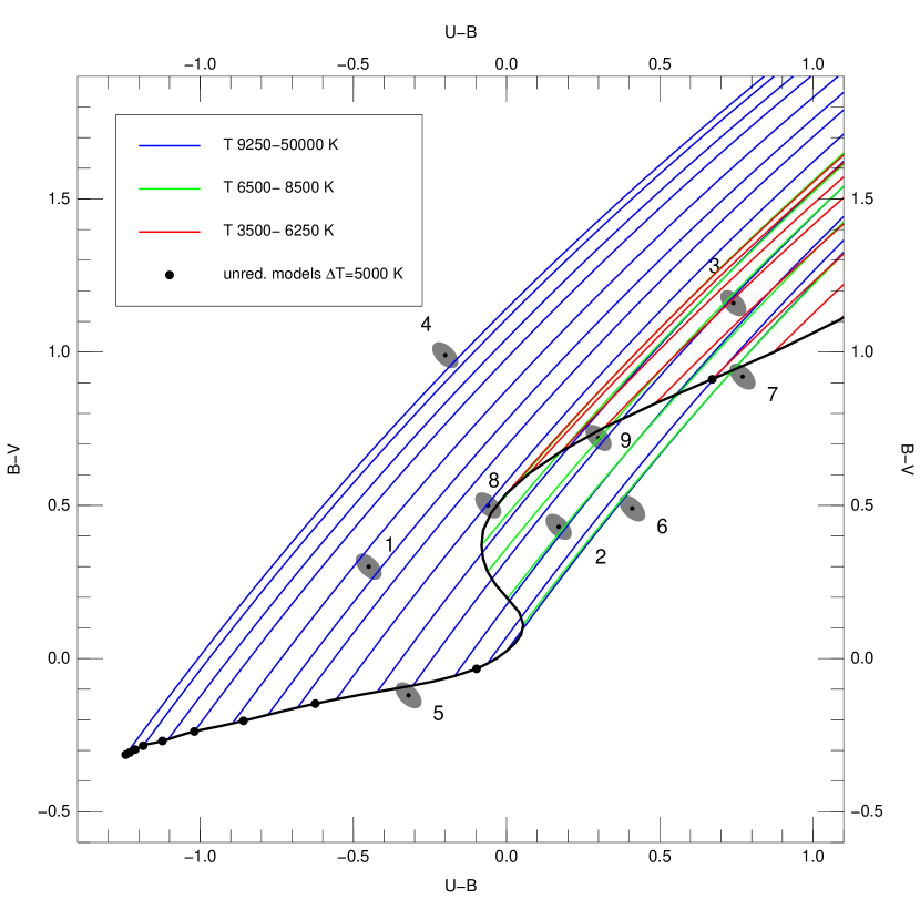
Figure 4.: $U-B$ vs. $B-V$ color-color plot for $Z=0.0$, main-sequence Kurucz atmospheric models. The line with circles indicates the location of the unredenned values as a function of temperature, starting at $T=50\,000$ K, with the circles marking those points where the temperature is a multiple of 5 000 K. The rest of the lines indicate the colors as a function of reddening using the Cardelli et al. (1989) law with $R_{5495}=3.1$, with the color code being used to differentiate among temperature ranges which are relevant to determine the number of possible temperature + reddening solutions for a given $(U-B)$ + $(B-V)$ combination. Nine measured stars are marked, each one of them with $\sigma_{U}=\sigma_{B}=\sigma_{V}=0.026$. Note that the reddening lines are not straight and that they are not parallel to each other because no Q-parameter approximation is used.

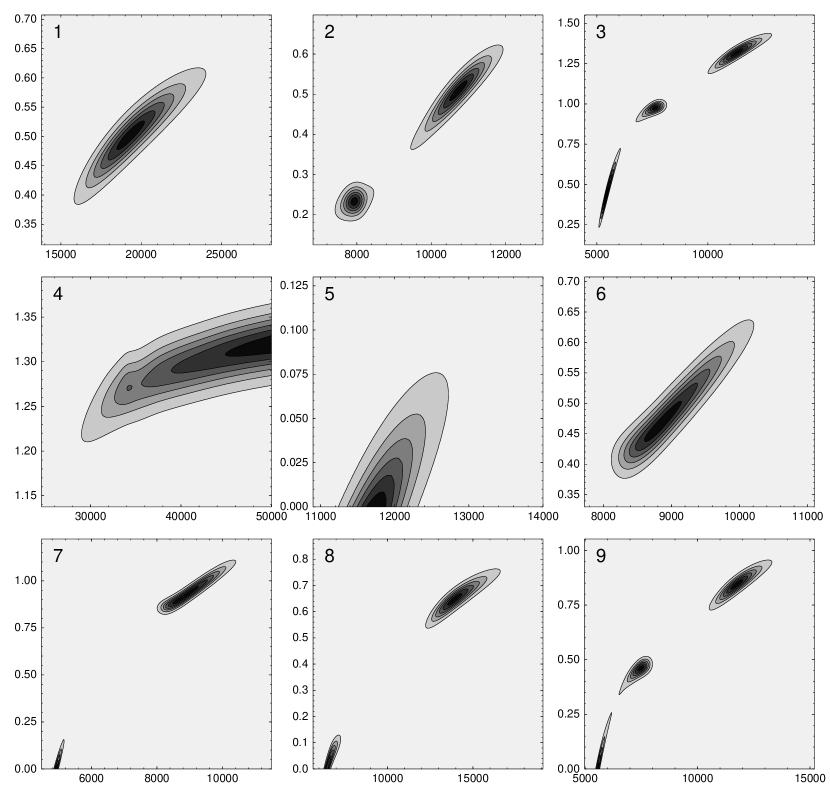
Figure 5.: Likelihood contour plots produced by CHORIZOS for the nine stars shown in Fig. 4. The $x$ axis corresponds to the temperature in K and the $y$ axis to the reddening $E(4405-5495)$.

 As previously mentioned, astronomers usually attempt to derive the $N$ parameters of individual stars (temperature, luminosity, metallicity, extinction…) or of stellar populations (age, metallicity, extinction…) by comparing the observed SCMDs with the synthetic magnitudes derived from SEDs. That is, they transform their model atmosphere outputs from the theoretical (or parameter) $N-dimensional$ space to an observational $M$-dimensional space with $M=2$ (one color and one magnitude) and compare the results with the data there. Such a strategy has a fundamental problems: if $N>2$, degeneracies are likely to exist, so a single solution cannot be obtained (this can happen even if $N=2$). Also, it is not straightforward to include information from an arbitrary number of additional colors: this is usually done by working on individual planes (e.g. projections onto two-dimensional observational space or color-color diagrams) but in doing so one loses the full multidimensional information. It is also common in such cases to use linearizing approximations, such as Q-ratio extinction corrections or filter transformations, hence introducing additional systematic errors (see Fig. 4).

An alternative is to use a code such as CHORIZOS (Maíz Apellániz 2004). CHORIZOS first calculates the theoretical colors for the full $N$-dimensional parameter space and then evaluates the likelihood in each point of the grid for the observed photometry. The moments of the resulting likelihood are then calculated to derive the range of possible parameters. Furthermore, since the code does not operate by simply finding a likelihood maximum (or $\chi^{2}$ minimum) it allows for the detection of multiple solutions. A simple example for the well-known case of finding the temperature and extinction ($N=2$) for stars of known metallicity and gravity and with a standard extinction law from Johnson $U-B$, $B-V$ colors ($M=2$) is shown in Figs. 4 and 5. Such an example has degeneracies, as it can be seen in the two possible solutions for e.g. star 2 and in the three possible solutions for e.g. star 3. Such degeneracies can be lifted by using additional colors (Fig. 6), which CHORIZOS can easily handle.

 

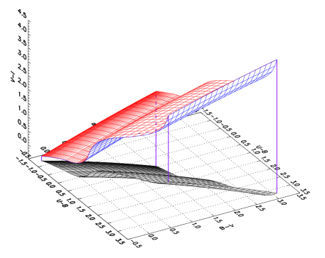
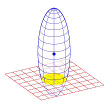
Figure 6.: (left) $V-I$ vs. $B-V$ vs. $U-B$ 3-color plot for $Z=0.0$, main-sequence Kurucz atmospheric models. The range plotted covers $T=3\,500-50\,000$ and $E(4405-5495)=0.0-2.0$ and the extinction law used is that of Cardelli et al. (1989) with $R_{5495}=3.1$. The color surface marks the location in 3-color space while the black one is the projection onto the $(U-B)$-$(B-V)$ plane (see Fig. 4). (right) Basic topology for an $M=3$, $N=2$ case such as the one on the left panel. Given that $M>N$, the measured colors (blue circle) always lies outside the solution surface (red grid). However, including the uncertainty ellipsoid (blue grid), yields an intersection surface (solid yellow) of likely solutions.

CHORIZOS is available to the astronomical community and can be downloaded from http://www.stsci.edu/~jmaiz. A number of upgrades to the code have been added since the publication of the original article (Maíz Apellániz 2004) and more are planned for the near future. We detail the current and future capabilities here:

CURRENT	FUTURE
SEDs: Kurucz, Lejeune, TLUSTY (stars); Starburst99 (clusters).	Arbitrary user-defined SED models for stars, clusters, galaxies…
Parameters: Up to four. Two SED-intrinsic ($T_{\rm eff}$ + log$g$, age) and two extrinsic (reddening + extinction law).	Five, user-defined and in any combination (metallicity, redshift, IMF slope, upper mass limit…).
Parameter control: Full range, restricted range, fixed. Grid size adjustable and extendable.	Use of Bayesian priors
Filters: 80 preinstalled (Johnson-Cousins, Strömgren, Tycho-2, SDSS, 2MASS, HST).	Future HST instruments?, user-defined.
Spectrophotometry: No.	Yes.

Eventually, CHORIZOS will become a full Bayesian code that will be able to handle any arbitrary SED family or filter set.

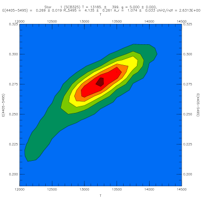
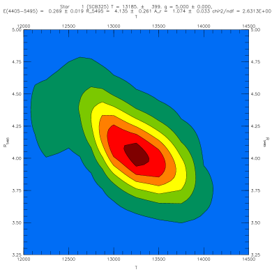
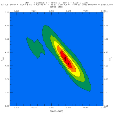
Figure 7.: Likelihood contour plots produced by CHORIZOS for one of the stars in the M8 sample. Each plot corresponds to the projection onto one of the 3 orthogonal planes defined using the three coordinates $T_{\rm eff}$, $E(4405-5495)$, and $R_{5495}$: $T_{\rm eff}-E(4405-5495)$ (upper left), $T_{\rm eff}-R_{5495}$ (lower left), and $E(4405-5495)-R_{5495}$ (lower right).

As an example of the possible applications of CHORIZOS to the study of stellar populations we include here a summary of the study performed by Arias et al. (2005). Those authors analyzed $UBVIJHK_{\rm s}$ photometry for six stars in the Galactic Hi̇i region M8. CHORIZOS was executed using solar-metallicity, main-sequence Kurucz stellar models with three free parameters: temperature, reddening, and extinction law. CHORIZOS parameterizes reddening by $E(4405-5495)$, the monochromatic equivalent of $E(B-V)$ and extinction law by $R_{5495}$, the monochromatic equivalent to $R_{V}$. The extinction laws of Cardelli et al. (1989) were used.

The likelihood plots for SCB 325, one of the six stars is shown in Fig. 7. CHORIZOS produces as graphical output the projection of the likelihood into each of the possible combinations of two free parameters (in this case, there are three free parameters, yielding three possible combinations). As it can be seen, the output is a well-defined peak with only a slight asymmetry, so the values of $T_{\rm eff}$, $E(4405-5495)$, and $R_{5495}$ and their uncertainties can be derived with confidence.

 

Figure 8.: Measured photometry and best-fit spectrum for Herschel 36 produced by CHORIZOS. The left plot shows the fit using all seven photometric bands ($UBVIJHK_{\rm s}$) while the right plot uses only the first five ($UBVIJ$). The corresponding values of the reduced minimum $\chi^{2}$ are 21 and 1.7, respectively. For the photometry, the vertical error bars are used to show the photometric uncertainties while the horizontal ones show the approximate extent of each filter in wavelength.

Another of the CHORIZOS outputs is shown in Fig. 8 for the case of Herschel 36, another star in the M8 sample. The left plot shows the best-fit spectrum when all seven photometric bands (six colors) are used. Such a best fit has a reduced $\chi^{2}$ of 21, indicating that the observed photometry is not compatible with the SED family and/or the parameter range used. A look at the plot immediately suggests the origin of the problem: the $UBVI$ photometry is apparently well fitted but the NIR data is not. As it turns out, Herschel 36 has a large IR excess, so a Kurucz model is not a good approximation for its SED in the NIR: CHORIZOS detects such circumstance by yielding a reduced minimum $\chi^{2}\gg 1$. If on the other hand, CHORIZOS is run excluding the $HK_{\rm s}$ photometry (right plot of Fig. 8), the result is very different: the reduced $\chi^{2}$ for the best fit is close to 1, as it is readily apparent from the concordance between the spectrum and the photometry (note that the two rightmost photometric points are not included in the fit).

Figure 9.: Theoretical ( $T_{\rm eff}$ vs. $M_{\rm bol}+5\log d-5$) HR diagram for the six stars in the M8 sample produced by CHORIZOS. Ellipses indicate the 68% likelihood contour for each star. The line shows the main sequence for $5\log d-5=10.5$. As seen in the plot, such a distance is compatible with the CHORIZOS output for the four earliest stars but not for the latest two.

Once the photometry of each star has been processed by CHORIZOS and the parameters ($T_{\rm eff}$, $E(4405-5495)$, $R_{5495}$) and their uncertainties have been evaluated, it is possible to construct the theoretical HR diagram (Fig. 9). Note that the uncertainty ellipses are inclined with respect to the two coordinates. The reason is the strong correlation between $T_{\rm eff}$ and $M_{\rm bol}$ induced by the dependence of the bolometric correction on temperature. The HR diagram shows that the photometry of the four earliest-type stars in the sample is compatible with a distance modulus of 10.5. The two late B stars, however, must be farther away, since their uncertainty ellipses fall clearly below the expected main sequence at that distance.

5. Conclusions

 I have shown the importance of the accurate calibration of photometric systems in order to produce meaningful comparisons between the observed colors and magnitudes and model SEDs. The Tycho-2 calibration derived by Bessell (2000) (for the sensitivity curves) and Maíz Apellániz (2005) (for the zero points) is precise enough for that task. On the other hand, the available calibrations for Johnson $UBV$ photometry yield relatively large systematic errors, which has prompted me to develop a new, more precise calibration. I have also shown how the use of multicolor photometry has significant advantages over the standard single-color + magnitude diagrams, among them the elimination of degeneracies, the inclusion of multiple parameters, the avoidance of linearizing approximations, and the possibility of a precise treatment of errors.

Acknowledgments.

I would like to thank Ralph Bohlin and Rodolfo Barbá for fruitful conversations about the topics discussed in this work.

References

- Arias et al. (2005) Arias, J. I., Barbá, R. H., Maíz Apellániz, J., Morrell, N. I., & Rubio, M. 2005, submitted to MNRAS
- Bessell (1990) Bessell, M. S. 1990, PASP, 102, 1181
- Bessell (2000) Bessell, M. S. 2000, PASP, 112, 961
- Bessell et al. (1998) Bessell, M. S., Castelli, F., & Plez, B. 1998, A&A, 333, 231
- Bohlin (2000) Bohlin, R. C. 2000, AJ, 120, 437
- Bohlin et al. (2001) Bohlin, R. C., Dickinson, M. E., & Calzetti, D. 2001, AJ, 122, 2118
- Bohlin & Gilliland (2004) Bohlin, R. C., & Gilliland, R. L. 2004, AJ, 127, 3508
- Buser & Kurucz (1978) Buser, R., & Kurucz, R. L. 1978, A&A, 70, 555
- Cardelli et al. (1989) Cardelli, J. A., Clayton, G. C., & Mathis, J. S. 1989, ApJ, 345, 245
- ESA (1997) ESA. 1997, The Hipparcos and Tycho Catalogues (ESA SP-1200)
- Gregg et al. (2004) Gregg, M. D., et al. 2004, American Astronomical Society Meeting Abstracts, 205
- Høg et al. (2000a) Høg, E., et al. 2000a, A&A, 357, 367
- Høg et al. (2000b) Høg, E., et al. 2000b, A&A, 355, L27
- Johnson (1966) Johnson, H. L. 1966, Ann. Rev. Astron. Astroph., 4, 193
- Maíz Apellániz (2004) Maíz Apellániz, J. 2004, PASP, 116, 859
- Maíz Apellániz (2005) Maíz Apellániz, J. 2005, PASP (June 2005 issue)
- Mermilliod et al. (1997) Mermilliod, J.-C., Mermilliod, M., & Hauck, B. 1997, A&AS, 124, 349
- STScI (1998) STScI. 1998, Synphot User’s Guide, Howard Bushouse and Bernie Simon (eds.)