Frequency dependence of the drifting subpulses of PSR B0031$-$07

The well known drifter PSR B0031$-$07 is known to exhibit drifting subpulses where the spacing between the drift bands ($P_{3}$) shows three distinct modes A, B and C corresponding to 12, 6 and 4 seconds respectively. We have investigated periodicities and polarisation properties of PSR B0031$-$07 for a sequence of 2700 single pulses taken simultaneously at 328 MHz and 4.85 GHz. We found that mode A occurs simultaneously at these frequencies, while modes B and C only occur at 328 MHz. However, when the pulsar is emitting in mode B at the lower frequency there is still emission at the higher frequency, hinting towards the presence of mode B emission at a weaker level. Further, we have established that modes A and B are associated with two orthogonal modes of polarisation, respectively. Based on these observations, we suggest a geometrical model where modes A and B at a given frequency are emitted in two concentric rings around the magnetic axis with mode B being nested inside mode A. Further, it is evident that this nested configuration is preserved across frequency with the higher frequency arising closer to the stellar surface compared to the lower one, consistent with the well known radius-to-frequency mapping operating in pulsars.

1 Introduction

The single pulses of a pulsar are known to be composed of several smaller units of emission called subpulses. These subpulses are often seen to drift in phase across a sequence of single pulses giving rise to the well-known phenomenon of ‘drifting subpulses’, discovered in 1968 (Drake & Craft 1968). The drift pattern is seen to repeat itself after a given time which is usually denoted by $P_{3}$. The phenomenon has since been detected in many pulsars (e.g. Rankin 1986) and the process is believed to carry information on the mechanism leading to coherent radio emission from pulsars. For example, Ruderman & Sutherland (1975) have suggested a vacuum gap model in which the subpulses correspond to beams of particles (or sparks) produced in the vacuum gap over the polar cap and are thought to rotate around the magnetic axis due to the perpendicular component of the electric field and the magnetic field ($E\times B$ drift). Measurements of the speed of rotation of subpulses might therefore give direct information on the electric field in the vacuum gap. Recently, Deshpande & Rankin (1999) have shown that drifting subpulses observed in PSR B0943+10 can be interpreted as 20 sparks rotating around the magnetic axis at a uniform speed.

Some pulsars show clear changes in the vertical spacing between drift bands ($P_{3}$): for example PSR B0809+74 shows a changing $P_{3}$ after it goes through a null (van Leeuwen et al. 2002). PSR B0031$-$07 is particularly interesting because it shows three distinct drift-modes with different $P_{3}$, which are all very stable. They are named mode A, B and C and correspond to a $P_{3}$ of 12, 6 and 4 seconds (or 13, 7 and 4 $P_{1}$), respectively. These values are approximations and from 40,000 pulses observed at 327 MHz Vivekanand & Joshi (1997) found that they may not be harmonically related. They also found that at 327 MHz the relative occurrence rate of these modes are 15.6%, 81.8% and 2.6%, respectively. Furthermore, the pulses occur in clusters containing 30 to 100 pulses which follow each other with delays ranging from fifty to several hundred pulse periods. These clusters are constituted in one of three ways: a series of A bands followed by B bands, only B bands, or a series of B bands followed by C bands (Huguenin et al. 1970; Wright & Fowler 1981). This pulsar also shows a clear presence of Orthogonally Polarised Modes (OPM) in the integrated position angle sweep (Manchester et al. 1975). Table 1 lists some of the known parameters of PSR B0031$-$07. The values for $\alpha$ and $\beta$ were found by fitting the single vector model from Radhakrishnan & Cooke (1969) to the position angle of the dominant polarisation mode. The $\alpha$ and $\beta$ values from the position angle of the remaining polarisation mode are the same within errors.

PSR B0031$-$07 has been thoroughly studied at low observing frequencies (Huguenin et al. 1970; Krishnamohan 1980; Wright 1981; Vivekanand 1995; Vivekanand & Joshi 1997, 1999; Joshi & Vivekanand 2000), but only rarely at an observing frequency above 1 GHz (Wright & Fowler 1981; Kuzmin et al. 1986; Izvekova et al. 1993). Wright & Fowler (1981) have observed PSR B0031$-$07 at 1.62 GHz and have found the same drift-modes as seen at lower frequencies. Kuzmin et al. (1986) have studied the integrated pulse profiles of PSR B0031$-$07 at 102.7 MHz, 4.6 GHz and 10.7 GHz. Izvekova et al. (1993) have studied the subpulse characteristics of PSR B0031$-$07 at 62, 102, 406 and 1 412 MHz. They found that the switching between the three drift-modes and the nulls occur simultaneously at all frequencies. In this paper we study the behaviour of the different modes of drift in PSR B0031$-$07 in radio observations at both low and high observing frequencies simultaneously. In Section 2 we explain how the observations have been obtained, how the different modes of drift have been determined, and what further analyses have been carried out. In Section 3 we present our results. The discussion follows in Section 4. In this last section we present a geometrical model which describes many of the observed characteristics of this pulsar.

Table 1: List of known parameters of PSR B0031$-$07.

Parameter	Value	Reference
$P_{1}$	0.94295 s	Taylor et al. (1993)
$\dot{P}$	$4.083\cdot 10^{-16}$	”
DM	10.89 pc cm-3	”
$S_{400}$	95 mJy	”
$S_{1400}$	11 mJy	”
$B_{surf}$	$6.31\cdot 10^{11}$ G	”
$\dot{E}$	$1.9\cdot 10^{31}$ erg/s	”
$\alpha$	4.5$\pm 1.0\degr$
$\beta$	+4.8$\pm 1.0\degr$

1.1 Definitions

To describe the observational drift of subpulses we use three parameters, which are defined as follows: $P_{3}$ is the spacing at the same pulse phase between drift bands in units of pulsar periods ($P_{1}$); this is the “vertical” spacing when the individual radio profiles obtained during one stellar rotation are stacked as in Fig. 1. $P_{2}$ is the interval between successive subpulses within the same pulse, given in degrees. $\Delta\phi$, the subpulse phase drift, is the time interval over which a subpulse drifts, given in $\degr$/$P_{1}$. Note that $P_{2}=P_{3}\times\Delta\phi$.

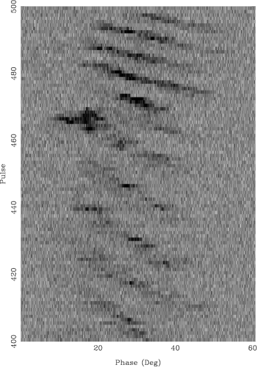
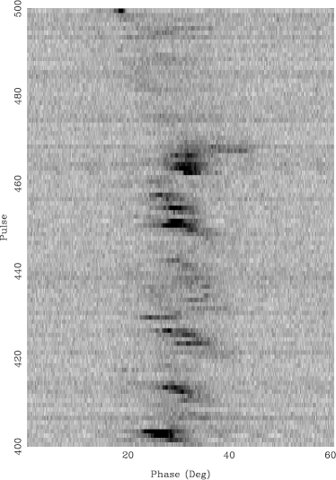
Figure 1: Gray scale plot of individual pulse profiles from the observation at 328 MHz (left) and 4.85 GHz (right) (pulse phase is plotted horizontally and pulse number vertically). These pulses show an example of a rapid mode change. The drift goes from mode A to mode B within a few pulses. It can also be seen that there is only a hint of mode-B drift in the 4.85-GHz observation.

2 Data analysis

The observations of PSR B0031$-$07, were obtained on 3 February 2002 with both the Westerbork Synthesis Radio Telescope (WSRT) and the Effelsberg Radio Telescope simultaneously. These observations were obtained as part of the MFO program. The WSRT observations were made at a frequency of 328 MHz and a bandwidth of 10 MHz. The Effelsberg observations were made at a frequency of 4.85 GHz and a bandwidth of 500 MHz. The time resolutions are 204.8 $\mu$s and 500 $\mu$s for the 328 MHz and 4.85 MHz observations, respectively. The 328-MHz observations have been corrected for Faraday rotation, dispersion and for an instrumental polarisation effects using a procedure described in the Appendix of (Edwards & Stappers 2004). Also, a 50-Hz signal present in the 4.85-GHz observation has been removed by Fourier transforming the entire sequence, removing the 50 Hz peak and Fourier transforming back. By correlating sequences of single pulses between the 328-MHz and 4.85-GHz observations that contained prominent subpulse drift the pulses could be aligned to within an accuracy of 2$\degr$ of pulse longitude, which confirms the broadband nature of the pulsar signal. This alignment is sufficient for the studies presented here.

We have also used an observation from PSR B0031$-$07, obtained on 9 August 1999 with the Effelsberg Radio Telescope at a frequency of 1.41 GHz and a bandwidth of 40 MHz. The time resolution is 250 $\mu$s.

2.1 Calculation of $P_{3}$

To search for periodicities, we considered a sequence of pulses from one of the observations. For each pulse in this sequence, we took the flux at a fixed phase, and calculated the absolute values of the Fourier transform of this flux distribution. This was done for each phase of the pulsar window. The resulting transforms were then averaged over phase, giving a phase-averaged power spectrum (PAPS) from 0 up to 0.5 cycles per rotation period (hereafter c $P_{1}^{-1}$), with a frequency resolution given by the reciprocal of the total length of the sequence.

Initially, all pulses from the observations were divided into sequences of 100 pulses, which were searched for peaks in the PAPS. When a peak was found, the beginning and end of the sequence was adjusted to get the highest signal-to-noise ratio for the peak. The signal-to-noise ratio was calculated as the peak value of the PAPS divided by the rms of the rest of the PAPS. This result was checked by visual inspection of the sequences to see whether they did indeed match the beginning and ending of a drift band. $P_{3}$ was then calculated as the reciprocal of the centre of the peak in the PAPS. When a peak would spread over multiple bins, a cubic spline interpolation was used to determine the location of the peak. The frequency resolution, given by the number of pulses in the sequence, was taken as the error on the position of the peak.

Furthermore, we have calculated the PAPS of all pulses of the 1.41- and 4.85-GHz observations in order to find signs of 6 second periodicity. For comparison, we also calculated the PAPS of the 328-MHz observation.

2.2 Values for $P_{2}$

Along with values for $P_{3}$, we also calculated the phase drift for each sequence of pulses. This was done by cross-correlating consecutive pulses. The fluxes in an interval around the peak of the cross-correlation were fitted with a Gaussian, from which the mean was taken as the phase drift. The error of the fit was taken as the error on the phase drift. $P_{2}$ was then determined by multiplying $P_{3}$ by the phase drift.

2.3 Average profiles and polarisation properties

To further study these distinct periodicities, we looked at the average-pulse profiles for the individual sequences of pulses that show mode A and mode-B drift, respectively. For the 4.85-GHz observation we compared the sequences that showed mode-A drift in the 4.85-GHz observation with the sequences that showed mode-B drift in the 328-MHz observation. In the same way, we calculated the average linear polarisation, circular polarisation and position angle as a function of pulse phase. We also measured the widths of the average total intensity at 10% and 50% of the peak values and at a height three times the rms. These analysis were done only for the 328-MHz and 4.85-GHz observations.

3 Results

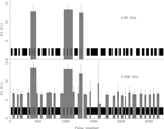
Figure 6: Sequences which show a periodicity of magnitude $P_{3}$ at fixed longitude (the gray areas). The lower panel shows the 328 MHz observation, while the upper panel shows the 4.85 GHz observation. The black lines indicate pulses which show a null at both frequencies.

The values of $P_{3}$ for each sequence and for both frequencies are shown in Fig. 6. Even though mode B does not seem to occur at 4.85 GHz, it should be noted that whenever mode B is active at 328 MHz there is always radiation present at 4.85 GHz. The same is true for mode C, but there is only one case of a mode C drift. Fig. 6 suggests that the transition between modes can happen within one or a few pulses. An example of how fast the drift-rate can change is shown in Fig. 1. In this figure the pulses are plotted from bottom to top. Mode A is present in the first five drift-bands. Then, within one or two pulses, the drift switches to mode B. In this example, it appears that the transition simply involves the appearance of a drift-band in a different mode, rather than the speeding up of the current drift-band. However, it should also be mentioned that this particular transition happens to occur exactly when a new drift-band would be expected to arise. In our observations there are only a few cases when there is a transition from one drift mode into the other without a null separating the two drift-bands. None of these transitions show a clear change of mode within one drift-band.

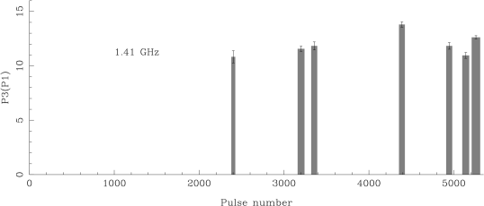
Figure 7: Sequences from the observation at 1.41 GHz which show a periodicity of magnitude $P_{3}$ at fixed longitude. The 1.41 GHz observation was not simultaneous with the other observations.

The values for $P_{3}$ from the observation at 1.41 GHz, are shown in Fig. 7. We found various examples of mode-A drift, but no mode-B drift. In this respect the 1.41-GHz observation resembles the 4.85-GHz observation. There are no drift-bands showing mode-C drift.

The PAPS of all three observations, are shown in Fig. 2. The low frequencies contain a signal due to the nulling. To make the figure clearer we have set them to zero. We see here that the 6-second periodicity is clearly present at 328-MHz and is just visible in the 1.41-GHz observation. At 4.85 GHz the PAPS does not show the 6-second periodicity. Thus, the mode-B drift gets weaker with increasing observing frequency. However, we did find small sequences in the 4.85-GHz observation where there is a weak 6-second periodicity. Fig. 3 shows the power spectrum of the flux as a function of pulse phase as well as the PAPS of a sequence of 20 pulses from the 4.85-GHz observation containing 6-second periodicity. The PAPS peaks at 6.6 seconds. We did not classify this as a mode-B drift, because the drift-bands are not clearly visible and the cross-correlation between consecutive pulses suggests the drift to be in the opposite direction of all the other drifts. It would be most difficult to explain a mode-B drift-band at high frequency that has a drift-direction different from the drift-direction of the same mode-B drift-band at low frequency. The present sequence is not significant enough to establish that this has occurred.

Figure 2: Phase averaged power spectra of three observations at frequencies of 4.85 GHz, 1.41 GHz and 328 MHz. There are clear signs of 6-seconds periodicity in the 1.41-GHz and 328-MHz observations. The dotted line is placed at 1/6.3 s

Figure 3: Contour plot of the power spectrum of the flux at 4.85 GHz as a function of pulse phase during a sequence with 6-second periodicity. The left panel shows the power spectrum integrated over longitude. The upper panel shows the power integrated over frequency. The 0 Hz peak has been put to 0.

Table LABEL:tab:P2 shows the average values for $P_{3}$, phase drift and $P_{2}$ for each drift-mode at three frequencies.

Fig. 8 shows the average-polarisation properties of pulses which show the same modes of drift. Each panel shows the total intensity (solid line), linear polarisation (dashed line), circular polarisation (dotted line) and position angle (lower half of each panel). The left panels show the 328-MHz profiles, the right panels show the 4.85-GHz profiles. The top panels show the average polarisation of pulses containing subpulses with mode-A drift, below that are the average polarisation of pulses containing subpulses with mode-B drift and the bottom panels show the average polarisation of all pulses. There is a clear 90$\degr$ jump in the position angles of all pulses in both the 328-MHz and 4.85-GHz profiles at a longitude of 24$\degr$. This jump can also be seen in the pulses that only show a mode-B drift. The widths of the average-intensity profiles are listed in Table 3.

Table 3: Widths of the average intensity profiles for different selections of pulses from the 328-MHz, 1.41-GHz and 4.85-GHz observations. The 1.41 GHz observation was not simultaneous with the other observations.

Frequency	Which pulses	10% width (deg)	50% width (deg)
328 MHz	Pulses in mode A ($P_{3}\approx 12\,s$)	37 $\pm$ 2	22.6 $\pm$ 1.1
328 MHz	Pulses in mode B ($P_{3}\approx 6\,s$)	42.2 $\pm$ 1.1	22.7 $\pm$ 0.4
328 MHz	All pulses	39.8 $\pm$ 1.1	24.0 $\pm$ 0.5
1.41 GHz	Pulses in mode A ($P_{3}\approx 12\,s$)	21.3 $\pm$ 1.8	8.8 $\pm$ 0.3
1.41 GHz	All pulses	29.9 $\pm$ 1.3	12.1 $\pm$ 0.5
4.85 GHz	Pulses in mode A ($P_{3}\approx 12\,s$)	24.6 $\pm$ 0.8	11.2 $\pm$ 0.3
4.85 GHz	Pulses in mode B ($P_{3}\approx 6\,s$)	33.5 $\pm$ 1.6	19.2 $\pm$ 0.5
4.85 GHz	All pulses	32.9 $\pm$ 0.9	16.1 $\pm$ 0.4

4 Discussion

We have analysed periodicities in two observations with 2700 pulses of PSR B0031$-$07 which were taken simultaneous at 328 MHz and 4.85 GHz. At low frequency we found that 61.8% of the time the pulsar was in one of the three drift-modes. The occurrence rate was 17.8% for mode A, 80.1% for mode B and 2.1% for mode C. This is consistent with previous results of Vivekanand & Joshi (1997). We have shown that whenever the mode-A drift is active, it is visible at both frequencies. Also, when the mode-B drift is active, it is clearly visible at 328 MHz, but not at 1.41 or 4.85 GHz (see Figs. 6 and 7). However, there is 6 second periodicity in the pulses at 1.41 GHz and a hint of 6 second periodicity in the pulses at 4.85 GHz, the latter of which is possibly drifting in the opposite direction of the drift observed at 328 MHz. This would suggest that towards higher frequency we are seeing less of the drifting subpulses and begin to see a diffuse component that is also subject to the $E\times B$ drift. It is difficult to explain a change in the direction of drift towards higher frequency while $P_{3}$ remains almost constant. It might indicate that the observed drift-rate is in fact an alias of the true drift-rate. Establishing and further investigating the possibility of a mode-B drift at 4.85 GHz with a drift direction opposite to that at 328 MHz might help determine the actual drift-rate and direction of the subpulses of this pulsar. The result that only one drift-mode is visible around 1.41 GHz differs from the results in Wright & Fowler (1981) and possibly differs from Izvekova et al. (1993).

In our observations we see that the drift-rate can change within one or two pulses, however we do not see any instance of a mode change within a drift-band. It should be noted that in most cases there is at least one null between two drift-bands with different drift-rates.

Table LABEL:tab:P2 shows that the $P_{2}$ of drift-modes A and B at 328 MHz is almost the same and that drift-mode C has a slightly smaller $P_{2}$ at this frequency. Within errors, however, our values agree with a constant $P_{2}$ for each drift-mode, unlike the behaviour predicted by Vivekanand & Joshi (1997), who claim that $P_{2}$ increases monotonically with $\Delta\phi$. With increasing frequency, the value of $P_{2}$ for polarisation mode A decreases, which can be explained by the decrease of the opening angle towards higher frequency, assuming radius-to-frequency mapping.

Fig. 8 shows that there is a distinct difference between the average profile of pulses with a 12-second periodicity (A-profile) and with a 6-second periodicity (B-profile). At 328 MHz, the A-profile seems to have two components. This can correspond to the line of sight cutting the edge of the subpulses in the centre of the profile, thereby bifurcating the average profile. It is interesting that the right component in the A-profile at 328 MHz seems to correspond to the single component of the A-profile at 4.85 GHz. Thus it appears as though the first component in the A-profile at 328 MHz disappears towards higher frequency. The profiles at 328 MHz also show that the intensity of the pulses in drift-mode A is on average lower than the intensity of the pulses in drift-mode B. A difference in average profile of the three modes has been reported before by Wright & Fowler (1981) and Vivekanand & Joshi (1997). The former authors have observed the pulsar at 1.62 GHz and found that the A-profile is more narrow than the B-profile, which is in turn more narrow than the C-profile. We cannot directly compare this result with our observation at 4.85 GHz as we do not see a mode-B drift at this frequency. But if we define the B-profile as the pulses at 4.85 GHz that show a mode-B drift at 328 MHz, then we find that at 4.85 GHz, the A-profile is indeed more narrow than the B-profile. Wright & Fowler (1981) do not note a difference in amplitude, nor an offset which are first noted by Vivekanand & Joshi (1997), who have observed the pulsar at 326.5 MHz. They show that at this frequency pulses in drift-mode B have on average more intensity than pulses in drift-mode A and C, which are of equal intensity. They also state that drift-mode A arrives earlier than drift-mode B, which in turn arrives earlier than drift-mode C. Both findings are confirmed by our results from the 328 MHz observation. However, they do not report a double component in the A-profile, which is indeed not present in their plot. This might be due to the fact that only a single linear polarisation was used in their observation. Table 3 shows that the widths from the average intensity profiles decreases from 328 MHz to 1.41 GHz and increases again from 1.41 to 4.85 GHz. This behaviour is not consistent with radius-to-frequency mapping. However, we should note that the signal-to-noise ratio of the edges of the profiles might not be high enough to detect the entire width of the pulse, which makes it difficult to draw any conclusions from these values. Furthermore, when we compare the change in 50%-width from the A-profile with the change in $P_{2}$ between 328 MHz and 4.85 GHz, we find that the value for $P_{2}$ decreases roughly by 65% while the width of the A-profile only decreases by 50%. Both should reflect the change in the size of the radioactive region due to radius-to-frequency mapping. To explain this discrepancy we suggest that at each frequency the drift-path of the subbeams is surrounded by an area of weak radio-emission which becomes relatively smaller with decreasing frequency. To support this claim we have constructed average intensity profiles with contributions from the mode-A drift-bands only. This was achieved by adding up the spectral power in the fluctuation spectrum in the domain between 0.07 and 0.1 Hz at each pulse phase. We then compared the 50%-widths of these profiles at 328 MHz and 4.85 GHz. We found that these widths were approximately 22$\degr$ and 7$\degr$, respectively, which is consistent with the change of $P_{2}$ between these frequencies.

Fig. 8 also shows that the average polarisation of all pulses from the 328-MHz observation has two components and a clear minimum around a pulsar phase of 24$\degr$. From the average polarisation of pulses at 328 MHz that are in drift-mode A and B, it is apparent that the pulses in drift-mode A contribute only to the component on the left and the pulses in drift-mode B contribute only to the component on the right. The average position angle of all pulses shows a 90$\degr$ jump at both frequencies at a pulsar phase of 24$\degr$. This can be interpreted as two orthogonally polarised modes changing dominance at this pulsar phase. A straight line fit to the position angles of both modes has shown that these polarisation modes are indeed 90$\degr$ apart. This jump is also visible in the average position angle of pulses that are in mode-B drift. We have searched for this jump in the average position angle of short sequences containing 20 to 50 pulses in a particular drift-mode and did not find a clear change in polarisation mode. It only manifests itself in the average of many sequences. Furthermore, the pulses in mode-A drift do not show any sign of a jump in position angle. They only show some degree of linear polarisation in the left part of the profile, just before the mode jump occurs in the average position angle of all pulses. Thus the left part of the A-profile is dominated by one of the two orthogonal polarisation modes, while the lack of polarisation in the right part of the A-profile suggests that here both polarisation modes are of equal strength. The lack of polarisation in the left part of the B-profile suggests that here both polarisation modes are also of equal strength, while the right part of the B-profile is dominated by the other polarisation mode. This means that there is a strong relationship between the drift-modes A and B and the two orthogonal modes of polarisation.

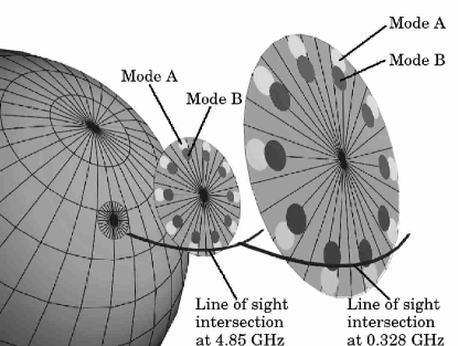
(a)	(b)

Figure 4: (a) Schematic overview of the proposed geometrical model to explain the absence of one mode at high frequency. The two large discs are centred around the magnetic axis and represent the emission region at two different frequencies, corresponding to two different altitudes above the pulsar surface. The smaller circles in the emission region represent the positions of the drifting subpulses, which rotate around the magnetic axis. The true number of subpulses is unknown. The different drift-modes are illustrated by different colours. Please note that only one drift-mode is assumed to be active at a time. (b) Schematics of two field lines from which radio waves of two different frequencies are observed. L is the line that connects the locations where the field lines are directed towards the observer. Due to radius-to-frequency mapping, low frequency radio waves are emitted from inner field lines with respect to those where the high frequency radiation is emitted for the same line of sight. This picture also illustrates that radio waves observed from outer field lines are emitted closer to the magnetic axis than radio waves from inner field lines. Thus, the width of the emission profile decreases with increasing frequency.

4.1 Modelling the observations

Since the limited length of our observations does not enable us to study mode C, we shall only attempt to model the behaviour of modes A and B, which are the most prominent drift-modes. We have found that of these two drift-modes only mode A is visible at high frequency, while at low frequency both modes are visible and are seen to have different orthogonal polarisation. At low frequency, the pulses in mode A have less intensity than the pulses in mode B, while at high frequency the pulses show the opposite behaviour. Furthermore, even though the mode B drift is not clearly visible at 4.85 GHz, we do see a hint of 6 seconds periodicity at this frequency. In the context of the potential gap model, the different rates of drift seem to suggest that the potential gap can take on different stable values. Each stable value can be associated with a particular drift rate and a particular magnetic surface of emission if we assume that the radiation is emitted tangential to the magnetic field lines. An increase in the value of the potential gap is expected to give rise to a faster drift and emission (pair production) from magnetic field-lines closer to the magnetic axis. This leads to the picture of an emission region with two concentric radiating rings. At high frequency, the line of sight intersects with magnetic field lines which are further away from the magnetic axis than at low frequency. Therefore, the drifting component of the inner ring is not seen at high frequency. This is graphically illustrated in Fig. 4.

Figure 5: Schematic overview of two models explaining the observed behaviour of two of the drift-modes of PSR B0031$-$07 at two frequencies f1, f2 (f1$<$f2). The left panel illustrates our present model. The right panel illustrates the model of van Leeuwen et al. (2003). As the pulsar rotates the line of sight passes from L3 over L2 to L1 and back. Emission at low frequency corresponds to altitudes P1, P2 (and P1’, P2’) whereas emission at high frequency comes from altitudes P3, P4 (and P3’, P4’).

It is also possible to construct a model wherein the emission of both modes comes from the same magnetic flux surface, but from different heights. Such a model is given in van Leeuwen et al. (2003). The difference between the two models is graphically illustrated in Fig. 5. Here, L1, L2 and L3 are the locations where the field lines are directed towards the observer for three different lines of sight: L1 when the line of sight is closest to the magnetic axis, L2 when the line of sight just touches the emission region when observing at high frequency, and L3 shows when the line of sight just touches the emission region when observing at low frequency. In case of a dipole magnetic field, the lines L1 - L3 are straight. Note that these lines do not lie in a plane as might be suggested by Fig. 5. Therefore, one must consider these images as lying in the plane through one of the three lines and the magnetic axis. At points on L1, L2 or L3 further away from the pulsar surface the curvature of the field lines decreases and the frequency of emission is believed to be lower.

In our model (left image) a mode change is caused by a shift of the emission to inner field-lines. At high frequency, the observer can only see emission coming from a region between points P3 and P4. As the mode changes from A to B, the observer will no longer see emission. At low frequency the observer can only see emission coming from a region between the points P1 and P2, and is thus able to see both modes. Note that when the line of sight is closest to the magnetic axis, mode A is not visible, thus causing a dip in the centre of the A-profile at low frequency.

In the model of van Leeuwen et al. (2003) (right image) the emission always comes from the same field-lines. Now however, the emission altitude at a fixed frequency decreases when the mode changes from A to B. This causes the observer to see emission from a point lower in the pulsar magnetosphere (indicated by an open dot and an apostrophe). At high frequency, the observer will only see emission coming from a region between P3 and P4 if the pulsar is emitting in mode A but none in mode B since the region between P3’ and P4’ is not part of the ’active’ (radiating) flux tube. Thus the observer will only see emission in mode A. At low frequency the observer will only see emission coming from a region between P1 and P2 if the pulsar is emitting in mode A and will only see emission in a region between P1’ and P2’ if the pulsar is emitting in mode B. Thus the observer will be able to see emission from both modes. Note that also in this model mode A is not visible at low frequency when the line of sight is closest to the magnetic axis.

In the case of PSR B0031$-$07 both models can explain the observed characteristics. It is therefore difficult to distinguish between them observationally, especially if observing at only one frequency. However, if we were to observe this pulsar at a large range of frequencies (preferably simultaneous) it should be possible to make quantitative statements as to favour one of the models.

On theoretical grounds, we find a possible inconsistency in the model of van Leeuwen et al. (2003) when applied to our observations. In their model, which follows the work of Ruderman & Sutherland (1975) and Melikidze et al. (2000), the transition from mode A to B occurs by a decrease in height of the voltage gap. As a result the altitude of emission decreases. However, the electric field also decreases and with it the speed of the $E\times B$ drift, contrary to what is observed. Of course, a possible explanation for this inconsistency could be that we are not seeing the actual drift-speed, but an alias. It should be noted that variation of drift speed can also happen due to temperature variation on the polar cap as suggested by Gil et al. (2003).

5 Conclusions

From an analysis of 2700 pulses from PSR B0031$-$07 taken simultaneously at 328 MHz and 4.85 GHz we found that from the three known drift-modes A, B and C of PSR B0031$-$07 only mode A is visible at high frequencies. We have constructed a geometrical model that explains how one drift-mode can disappear at high frequency while another drift-mode remains visible. Further, we have shown that the two most prominent drift-modes A and B are associated with two orthogonal modes of polarisation, respectively. To continue the study presented here, one would require more multi-frequency single pulse observations from this pulsar containing full Stokes parameters.

Figure 8: Average intensity and polarisation of pulses in mode A (top panels), pulses in mode B (middle panels) and all pulses (lower panels). The profiles have been normalised to set the peak in the average intensity of all pulses to 1. The left panels show the average of pulses at 328 MHz, the right panels show the average of the same pulses at 4.85 GHz. Since the pulses at 4.85 GHz do not show a mode-B drift, the right middle panel contains the average of pulses at 4.85 GHz that show a mode-B drift at 328 MHz. The solid, dashed and dotted lines in each panel represent the total intensity, linear polarisation and circular polarisation, respectively. The lower part of the panels show the polarisation position angle. The 328 MHz profiles have been re-binned to 500 $\mu$s per bin, to make the profiles comparable.