An Efficient Numerical Scheme for Simulating Particle Acceleration in Evolving Cosmic-Ray Modified Shocks
Abstract
We have developed a new, very efficient numerical scheme to solve the CR diffusion convection equation that can be applied to the study of the nonlinear time evolution of CR modified shocks for arbitrary spatial diffusion properties. The efficiency of the scheme derives from its use of coarse-grained finite momentum volumes. This approach has enabled us, using momentum bins spanning nine orders of magnitude in momentum, to carry out simulations that agree well with results from simulations of modified shocks carried out with our conventional finite difference scheme requiring more than an order of magnitude more momentum points. The coarse-grained, CGMV scheme reduces execution times by a factor approximately half the ratio of momentum bins used in the two methods. Depending on the momentum dependence of the diffusion, additional economies in required spatial and time resolution can be utilized in the CGMV scheme, as well. These allow a computational speed-up of at least an order of magnitude in some cases.
keywords:
, url]www.astro.umn.edu/twj
1 Introduction
Collisionless shocks are widely thought to be effective accelerators of energetic, nonthermal particles (hereafter Cosmic-Rays or CRs). Those particles play central roles in many astrophysical problems. The physical basis of the responsible diffusive shock acceleration (DSA) process is now well established through in-situ measurements of heliospheric shocks [10, 11] and through analytic and numerical calculations [3, 6, 7, 25, 31]. While test particle DSA model treatments are relatively well developed; e.g., [7, 32], it has long been recognized that DSA is an integral part of collisionless shock physics and that there are substantial and highly nonlinear backreactions from the CRs to the bulk flows and to the MHD wave turbulence mediating the CR diffusive transport (see, for example, [31] and references therein). Most critically, the CRs can capture a large fraction of the kinetic energy dissipated across such transitions. As they diffuse upstream the CRs form a pressure gradient that decelerates and compresses the entering flow inside a broad shock precursor. That, in turn, can lead to greatly altered full shock jump conditions, especially if the most energetic CRs, which can have very large scattering lengths, escape the system and carry significant energy with them. Also in response to the momentum dependent scattering lengths and flow speed variations through the shock precursor the CR momentum distribution will take on different forms than in a simple discontinuity. Effective analytic (e.g., [5, 6, 28]) and numerical (e.g., [9]) methods have been developed that allow one to compute steady-state modified shock properties given an assumed diffusion behavior. On the other hand, as the CR particle population evolves in time during the formation of such a shock the shock dynamics and the CR-scattering wave turbulence evolve as well. For dynamically evolving phenomena, such as supernova remnants, the time scale for shock modification can be comparable to the dynamical time scales of the problem.
The above factors make it essential to be able to include both nonlinear and time dependent effects in studies of DSA. Generally, numerical simulations are called for. Full plasma simulations offer the most complete time dependent treatments of the associated shock microphysics [14, 35], but are far too expensive to follow the shock evolution over the time, length and energy scales needed to model astrophysical CR acceleration. The most powerful alternative approach utilizes continuum methods, with a kinetic equation for each CR component combined with suitably modified compressible fluid dynamical equations for the bulk plasma (see §2 below). By extending that equation set to include relevant wave action equations for the wave turbulence that mediates CR transport, a self-consistent, closed system of equations is possible (e.g., [1, 2, 17, 18])). Continuum DSA simulations of the kind just described are still quite challenging and expensive even with only one spatial dimension. The numerical difficulty derives especially from the very large range of CR momenta that must be followed, which usually extends to hundreds of GeV/c or beyond on the upper end and down to values close to those of the bulk thermal population, with nonrelativistic momenta. The latter are needed in part to account for “injection” of CRs due to incomplete thermalization that is characteristic of collisionless shocks.
One computational constraint comes from the fact that CR resonant scattering lengths from MHD turbulence, , are generally expected to be increasing functions of particle rigidity, . The characteristic length coupling the CRs of a given momentum, , to the bulk flow and defining the width of the modified shock precursor is the so-called diffusion length, , where is the CR particle speed, and is the bulk flow speed into the shock. One must spatially resolve the modified shock transition for the entire range of in order to capture the physics of the shock formation and the spatial diffusion of the CRs, in particular. The relevant typically spans several orders of magnitude, beginning close to the dissipation length of the thermal plasma, which defines the thickness of the classical, “viscous” gas shock, also called the “subshock” in modified structure. This resolution requirement generally leads to very fine spatial grids in comparison to the “outer scale” of the problem, which must exceed the largest .
Two approaches have been applied successfully so far to manage this constraint in DSA simulations. Berezhko and collaborators [3] developed a method that normalizes the spatial variable by at each momentum value of interest during solution of the CR kinetic equation. This approach establishes an spatial grid that varies economically in tune with . Derived CR distribution properties at different momenta can be combined to estimate feed-back on the bulk flow at appropriate scales. The method was designed for use with CR diffusion properties known a priori. It is not readily applied to CR diffusion behaviors incorporating arbitrary, nonlinear feedback between the waves and the CRs. As an alternative that can accommodate those latter diffusion properties, Kang et al.[24] have implemented diffusive CR transport into a multi-level adaptive mesh refinement (AMR) environment. The benefit of AMR in this context comes from the feature that the highest resolutions are only necessary very close to the subshock, which can still be treated as a discontinuity satisfying standard Rankine-Hugoniot relations. By efficient use of spatial gridding both of these computational strategies can greatly reduce the cost of time dependent DSA simulations.
On the other hand, the above methods do not directly address the principal computational cost in such simulations, so they remain much more costly compared to purely hydrodynamic or MHD simulations. This is because the dependence of on CR momentum, , adds a physical dimension to the problem. In practice, the spatial evolution of the kinetic equation for each CR constituent must be updated over the entire spatial grid at multiple momentum values; say, . The value of is usually large, since the spanned range of CR momentum is typically several orders of magnitude. Physically, CRs propagate in momentum space during DSA in response to adiabatic compression in the bulk flow, sometimes by momentum diffusion (see, for example, equation 1 below), or because of various irreversible energy loss mechanisms, such as Coulomb or radiative losses. The associated evolution rates for depend on the process, but generally depend on . The conventional approach to evolving approximates through low order finite differences in (e.g., [3, 12]). Experience has shown that converged solutions of using such methods require [3, 21]. In that case, for example, a mere five decades of momentum coverage requires more than 100 grid points in . Since spatial update of the kinetic equation at each momentum grid point requires computational effort comparable to that for any of the accompanying hydrodynamical equations (e.g., the mass continuity equation), CR transport then dominates the computational effort by a very large factor, commonly exceeding an order of magnitude.
An attractive alternative approach to evolving the kinetic equation replaces by its integral moments over a discrete set of finite momentum volumes, in which case is replaced by evaluated at the boundaries of those volumes. The method we outline here follows that strategy. Because is relatively smooth, simple subvolume models can effectively be applied over moderately large momentum volumes. We have found this method to give accurate solutions to the evolution of with an order of magnitude fewer momentum bins than needed in our previous finite difference calculations. The computational effort to evolve the CR population is thereby reduced to a level comparable to that for the hydrodynamics. In recognition of its distinctive features we refer to the method as “Coarse-Grained Momentum finite Volume” or “CGMV”. It extends related ideas introduced in [19], [20] and [33] for test particle CR transport. Those previous presentations, while satisfactorily following CR transport in many large-scale, smooth flows, did not include spatial or momentum diffusion, so could not explicitly follow evolution of during DSA. Instead, analytic, test-particle solutions for were applied at shock jumps. Here we extend the CGMV method so that it can be applied to the treatment of fully nonlinear CR modified shocks.
We outline the basic CGMV method and its implementation in Eulerian hydrodynamics codes in §2. Several tests are discussed in §3, and our conclusions are presented in §4.
2 The Method
2.1 Basic Equation
The standard diffusion-convection form of the kinetic equation describing the evolution of the isotropic CR distribution function, , can be written in one spatial dimension as (e.g., [34]).
| (1) |
where is the bulk flow speed, , is the spatial diffusion coefficient, is the momentum diffusion coefficient, and is a representative source term. We henceforth express particle momentum in units of , where is the particle mass. The first RHS term in equation (1) represents “momentum advection” in response to adiabatic compression or expansion. For simplicity of presentation equation 1 neglects for now propagation of the scattering turbulence with respect to the bulk plasma, which can be a significant influence when the sonic and Alfvénic Mach numbers of the flow are comparable. Although it is numerically straightforward to include this effect, the details are somewhat complex, so we defer that to a follow-up work focussed on CR transport in MHD shocks.
Full solution of the problem at hand requires simultaneous evolution of the hydrodynamical flow, as well as the diffusion coefficients, and . Again postponing full MHD, the added equations to be solved are the standard gasdynamic equations with CR pressure included. Expressed in conservative, Eulerian formulation for one dimensional plane-parallel geometry, they are
| (2) |
| (3) |
| (4) |
where and are the isotropic gas and the CR pressure, respectively, is the total energy density of the gas per unit mass and the rest of the variables have their usual meanings. The injection energy loss term, , accounts for the energy of the suprathermal particles transferred at low energy to the CRs. As usual, CR inertia is neglected in such computations, since the mass fraction of the CRs is generally tiny. We note for completeness that can be computed from using the expression
| (5) |
In the simulations described below we set the particle mass, , for convenience .
2.2 The CGVM Method
As mentioned in §1, the momentum advection and diffusion terms in equation 1 typically require when using low order finite difference methods in the momentum coordinate [3, 21]. The resulting large number of grid points in makes finding the solution of equation 1 the dominate effort in simulations of DSA. On the other hand, previous studies of DSA as well as direct observations of CRs in different environments have shown that is commonly well described by the form , where , is a slowly varying function of . Thus, we may expect a piecewise powerlaw form to provide an efficient and accurate, two-parameter subgrid model for . Two moments of are sufficient to recover the subgrid model parameters. We find it convenient to use
| (6) |
and
| (7) |
The first of these moments, , is proportional to the spatial number density of CRs in the momentum bin , while for relativistic CRs, is proportional to the energy density or pressure contribution of CRs in the bin. Then, for example,
| (8) |
where , and with obvious extension to . Either of these moments, plus their ratio, , can be used in straightforward fashion (e.g., iteration) to find both and the intrabin index, .
To evolve and we need the associated moments of equation 1 over the finite momentum volume bounded by . The result for is
| (9) |
where is a flux in momentum space, with , and where and are averaged over the momentum interval, according to
| (10) |
and
| (11) |
Extension of the momentum flux term to include other processes such as radiative or Coulomb losses is obvious (e.g., [19]). In practice these fluxes should be upwinded according to the signs of and . Evaluation of and at the boundaries of the included momentum range requires application of suitable boundary conditions, of course. We usually have set . In most cases we pick a sufficiently large maximum momentum, , that this condition is important only late in the simulation, if at all. Appropriate conditions at the lowest momenta can be more involved, depending on how one intends to connect the CR particle distribution to the thermal particle distribution, as in the injection models discussed below.
The -associated moment of equation 1 is
| (12) |
where ,
| (13) |
, and is given by an analogous expression to equation 11.
We note that momentum binning in the CGMV scheme is quite flexible, so that it can be easily adapted to either uniform or nonuniform momentum bin sizes, or to a momentum range that evolves during the simulation. We have successfully implemented both nonuniform and evolving momentum bin structures, although, for brevity we do not illustrate them here.
To update the distribution function we simultaneously integrate equations (9) and (12) over the timestep . Our implementation applies these methods in Eulerian hydrodynamical codes, so we split the update into two parts. Spatial advection is carried out by a second order, explicit van Leer scheme. The remaining terms are evolved using a second-order, semi-implicit Crank Nicholson scheme. For example, given values at timestep , and assuming for illustration a uniform spatial grid, the implicit part of the solution is given by the tridiagonal system
| (14) |
where
with , and .
The coefficients in equation 14 are obtained with the aid of the solutions to equations 2 - 4, which are updated prior to solution of equations 9 and 12. We note again that similar methods can be applied to follow the evolution of the wave turbulence that resonantly scatters CRs and that defines the spatial and momentum diffusion coefficients. In that case one begins with the wave action equation for the appropriate waves rather than the particle kinetic equation (e.g., [2]).
The solution of equation (14) for either or is quite analogous to our previous FD methods. Thus, since the CGMV method evolves two quantities rather than one, the relative effort required for a given is roughly twice in the CGMV scheme that required in the FD scheme. Our tests confirm this expected scaling. On the other hand, since can be dramatically reduced in a CGMV simulation the method can still be more efficient by a large factor.
2.3 A Flux Fraction Injection model
The most common source term represented by in equation (1) is injection at the shock of low energy CRs from the thermal plasma. There is presently no generally accepted theory for that process. However, we have implemented two commonly used models successfully into the CGMV scheme. For completeness we outline those here.
The simplest and one of the most frequently applied injection models assumes that a small, fixed fraction of the thermal particle flux through the gas subshock, , is injected at a momentum , where is a constant greater than unity and is the plasma sound speed immediately downstream of the subshock (e.g., [21]). This gives , where is the plasma mass density just upstream of the subshock, is the plasma mean particle mass, is the subshock speed with respect to the plasma immediately upstream and is a normalized weight function that allows the injection to be distributed across the numerical shock structure. In this case , while in the momentum bin with . Both and are zero, otherwise. The energy extracted from the thermal plasma is simply . For convenience we call this injection model the “flux fraction” or “FF” model.
2.4 A Thermal Leakage Injection model
A more sophisticated approach to injection physics includes models of the physical processes moderating particle orbits in the post shock flow region in order to estimate the probability that particles of a given speed will be able to escape back upstream, across the subshock. In such “thermal leakage” (TL) models for CR injection at shocks, most of the downstream thermal protons are locally confined by nonlinear MHD waves and only particles well into the tail of the postshock Maxwellian distribution can leak upstream across the subshock. In particular, “leaking” particles not only must have velocities large enough to swim against the downstream flow in order to return across the shock, they must also avoid being scattered during that passage by the MHD waves that mediate the plasma subshock. To model TL injection we utilize a “transparency function”, , expressing the probability that supra-thermal particles at a given velocity can leak upstream from behind the subshock (see [15] for details). In particular we set
| (15) |
where is the postshock flow speed in the subshock frame, is the Heaviside step function, and the particle velocity is normalized to . The parameter, , measures the ratio of the amplitude of the postshock MHD wave turbulence to the general magnetic field aligned with the shock normal, . Both hybrid simulations and theory suggest that [30], so that the model is well constrained. With this the shock is completely “opaque” to particles with momenta less than , i.e., for , where . So is the lowest momentum of the first momentum bin in the TL model and changes in time with the postshock flow speed. For , . The shock becomes virtually transparent to particles with momenta two to three times greater than . For strong, unmodified shocks in the TL model and in the FF model are similar when and . Under those circumstances the initial injection rates will be roughly similar, although differences in model physics lead to different behaviors as such shocks become modified (see, e.g., [4], [15], [25]).
The TL model is implemented in the CGMV scheme by the following numerical approach. After solution of equations (9) and (12) the net changes in and are corrected (reduced) in the upstream region by application of the transparency function as follows:
| (16) |
and
| (17) |
where , found using equation (8), is the CR distribution updated with equations (9) and (12). The energy loss rate of the bulk plasma to injection into the -th CR momentum bin can be approximated by
| (18) |
(see [25]).
3 Discussion
In order to test the performance of the new CGMV scheme we have installed it into two distinct one-dimensional Eulerian hydrodynamic (HD) codes that we have previously applied to studies of CR-modified shocks using conventional finite difference (FD) methods to solve the diffusion convection equation. In this section we briefly discuss the results and compare the CGMV and FD behaviors. Both of the host HD codes are constructed from high order, conservative Riemann solver-based schemes designed to capture shocks sharply. First we describe results from the CGMV scheme installed in a second order “Total Variation Diminished” (TVD) HD code based on the finite difference scheme of Harten [16]. This is the HD version of the MHD-CR code used by us in a previous study of CR modified shocks [23]. Gas subshocks in the TVD scheme typically spread over 2-3 numerical zones. An outline of the code mechanics and the FD CR scheme can be found there, in [13, 21] and references cited in those papers. The FD solver employed a Crank-Nicholson routine originally introduced in [12] for evolving that is similar to equation (14). For the TVD tests we applied the FF injection model.
In addition we present CGMV tests carried out with our Cosmic Ray Adaptive refinement SHock (CRASH) code. CRASH is based on the high order Godunov-like shock tracking algorithm of LeVeque [27]. The hydrodynamics routine in that code employs a nonlinear Riemann solver to follow shock discontinuities within the zones of an initially uniform grid. Thus, gas subshocks in CR-modified shocks remain discontinuous throughout a simulation, allowing CR transport to be modeled down almost to the scale of the physical shock thickness. CRASH also employs adaptive mesh refinement (AMR) around shocks in order to reduce the computational effort on the spatial grid. Refinement is centered on the subshock and each level spans 100 zones with a resolution twice as fine as the level above it. The number of refinement levels depends on what is required to capture diffusion of the lowest energy CRs. The standard, previously documented version of CRASH uses the same FD methods as the TVD code to solve the diffusion convection equation for CR transport. It is described in [24] and [25]. For the CRASH tests discussed in this paper we employed the TL injection model.
3.1 TVD-CR Tests
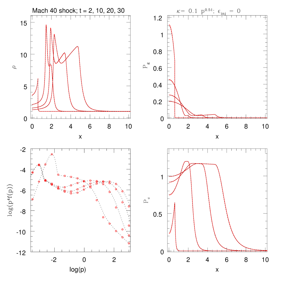
We first examine some results obtained using the TVD-CR code with both FD and CGMV schemes used to model the evolution of a strong CR-modified shock. Fig. 1 and Fig. 2 illustrate the evolution of shocks formed by the reflection of a Mach 30 flow (adiabatic index, ) off the left grid boundary. The resulting piston-driven shock initially has a Mach number, . The density and sound speed of plasma entering from the right boundary were set to and , respectively, so that the inflow speed was unity. The time unit for the calculations is also set by these scalings. In order to relate hydrodynamical variables to CR momenta it is necessary to fix the unit flow speed (the inflow speed in all the simulations discussed in this paper) with respect to the speed of light; i.e., . We set in the TVD-CR simulations. Time steps were fixed by a standard Courant condition, .
For the simulation illustrated in Fig. 1 evolution of the CR distribution is followed over the momentum range (). The simulation represented in Fig. 2 included the momentum range ().
The CR diffusion coefficient, is spatially uniform and set to . In a quest for a reasonably generalized behavior that required minimal computational effort, this choice was motivated by results from Malkov, who found self-similar analytic steady-state solutions for strong CR-modified shocks that apply to all powerlaw forms of , so long as the powerlaw index is steeper that [29]. Thus, our choice leads to fairly general shock behaviors in a way that minimizes the width of the precursor. That width, which determines the minimum space that must be simulated ahead of the subshock, is set by , where represents the maximum momentum contained. The TVD-CR simulations utilize a uniform, fixed grid, so, for example, the Bohm diffusion form modeled in the CRASH simulations below would lead to excessive costs for the TVD-CR FD test simulations presented in this section. The spatial resolution required for the calculations is set by , since accurate solutions of the diffusion-convection equation require good structural information in the diffusive shock precursor upstream of the subshock. Previous convergence tests have shown that is desirable (e.g., [21]). For the problems illustrated in Fig. 1 and Fig. 2 these considerations led us to set for both the FD and CGMV simulations. By varying this resolution, we verified that the shock evolution is reasonably converged with respect to .
The simulation followed in Fig. 1 assumes a pre-existing CR population, , corresponding to an upstream CR pressure, . No fresh injection is included at the shock; i.e., . This test then provides a simple and direct comparison between the CGMV and FD schemes for solving the diffusion-convection equation, since it omits any complications related to the injection model.
This simulation pair evolves the shocks until , which is sufficient to accelerate CRs to ultrarelativistic momenta. The spatial grid spans the interval [0,16], which is sufficient to contain the leading edge of the CR precursor to the end of the simulation.
The CR-modified shock spatial structures and the CR momentum distributions at the subshock are shown in Fig. 1 at times . Before comparing the solutions obtained with the two different methods, it is useful to summarize briefly the physics captured during the shock evolution. All the behaviors described here have been reported previously by multiple authors. The figure shows the well-known property of strongly modified shocks that the CRs extract most of the energy flux into the structure. That leads to a substantial drop in the postshock gas pressure, , and a large increase in the postshock density, . Together those indicate a strongly reduced postshock gas temperature. The decreased temperature is evident in the plot at the subshock, which is dominated at low momenta by the Maxwellian distribution of the bulk plasma. As CRs diffuse upstream against the inflowing gas they compress the flow within the precursor, preheating the gas (adiabatically in these simulations). Initially, while the CR pressure is relatively small compared to the incoming momentum flux, the gas subshock remains strong enough to produce a full four times density compression on top of the precompression. However, the subshock weakens once , reducing the subshock compression in this case to a factor , corresponding to a subshock Mach number near 2.3. That evolution explains the well-known, transitory “density spike” in the shock structures seen after . We note that since energy extracted from the flow by CRs becomes increasingly spread upstream and downstream due to CR diffusion, the total compression in such an evolving modified shock would always exceed the factor of seven one would predict for a strong, fully relativistic gas shock. For this simulation no significant CR energy escapes the spatial grid through upstream diffusion. However, at late times () the partial pressure due to CRs just below is sufficient that escape across the upper momentum boundary is significant. This contributes to the slow decrease in behind the shock and the increasing total compression through the shock transition that is visible in Fig. 1.
In the early evolutionary stages of this flow, while shock modification is modest, the CR momentum distribution resembles the powerlaw form, , predicted by test particle theory for a strong shock (e.g., [7]). With the spatial diffusion coefficient used in this simulation the high momentum cutoff to the distribution increases with time approximately as (see, e.g., [26]). As shock modification intensifies, most of the flow compression shifts from the subshock to the precursor. Then DSA of high momentum CRs occurs predominantly within the precursor rather than near the less important subshock. Consequently the CR distribution develops the familiar upwards-concave form resulting from the momentum dependent CR diffusion length. CRs of higher momentum experience a greater velocity jump within the precursor, so gain more energy each time they are reflected within the shock structure. That flattens the distribution, at momenta below . The result is a bump in the distribution of . On the other hand, CRs with momenta only a little above the injection range remain trapped close to the subshock. Their distribution closely approaches the steady state, powerlaw, test particle form appropriate to the weakened subshock. That feature extends upwards in momentum as the bump near moves upwards.
Looking finally to compare the two methods used to evolve the shock evolution displayed in Fig. 1 we see results from the FD scheme with and the CGMV scheme with . The agreement is generally very good. All the dynamical quantities, including shock jumps and the CR momentum distributions show excellent agreement. The curves representing the FD and CGMV distributions of , and and virtually indistinguishable in the plots. Most notably, all features formed in the FD evolution of the CR momentum distribution are faithfully reproduced by the much coarser CGMV distribution.
Given the excellent comparison in this strongly modified flow it is satisfying to note that the execution time required for the CGMV solution was a little less than 20% of that for the FD solution, demonstrating the significantly higher efficiency of the former method. The speed-up observed in our implementations of the two methods is roughly in accordance with what we would predict for a given reduction factor in the number of momentum values used, since the CGMV method requires one to evolve two distributions and for each momentum bin. We address convergence with respect to momentum resolution in our discussion of a second shock.
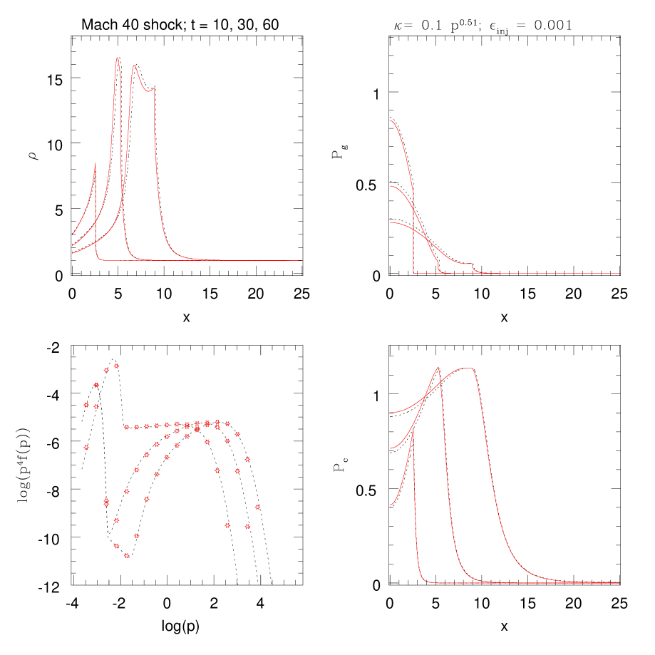
Fig.2 shows a Mach 30 flow similar to that in Fig. 1. In this case FF injection is included with commonly assumed values, and (see §2.3), the upper momentum bound is increased to and the spatial grid extends farther from the piston to . A negligible pre-existing CR population is included to avoid numerical issues coming from the fact that our CGMV scheme requires computation of the ratio over the entire grid.
The simulations evolved the shock until , which leads to . The spatial grid, spanning the interval [0,25], is sufficient to contain the CR leading edge of the precursor almost to the end of the simulations. However, after some CR energy escapes through the right boundary, due to diffusion upstream, mimicking the behavior of a “free escape” boundary (FEB) (e.g., [22] and references therein). Just as for the shock simulated in Fig.1, this energy loss amounts to a cooling process, so that the total shock compression increases with time as the simulation ends.
Again the agreement between FD and CGMV simulations is very good. Very early in the evolution of the shock, when the CRs are dominated by freshly injected nonrelativistic particles, the shock evolution is slightly faster in the CGMV scheme. That influence becomes insignificant later on, so that the modified shock structures found by the two schemes are almost identical as is the distribution at the shock. There is a small residual effect that the position of the subshock in the CGMV simulation lags slightly behind that of the FD simulation, and that is slightly higher in the CGMV simulation near the piston, where the shock first formed.
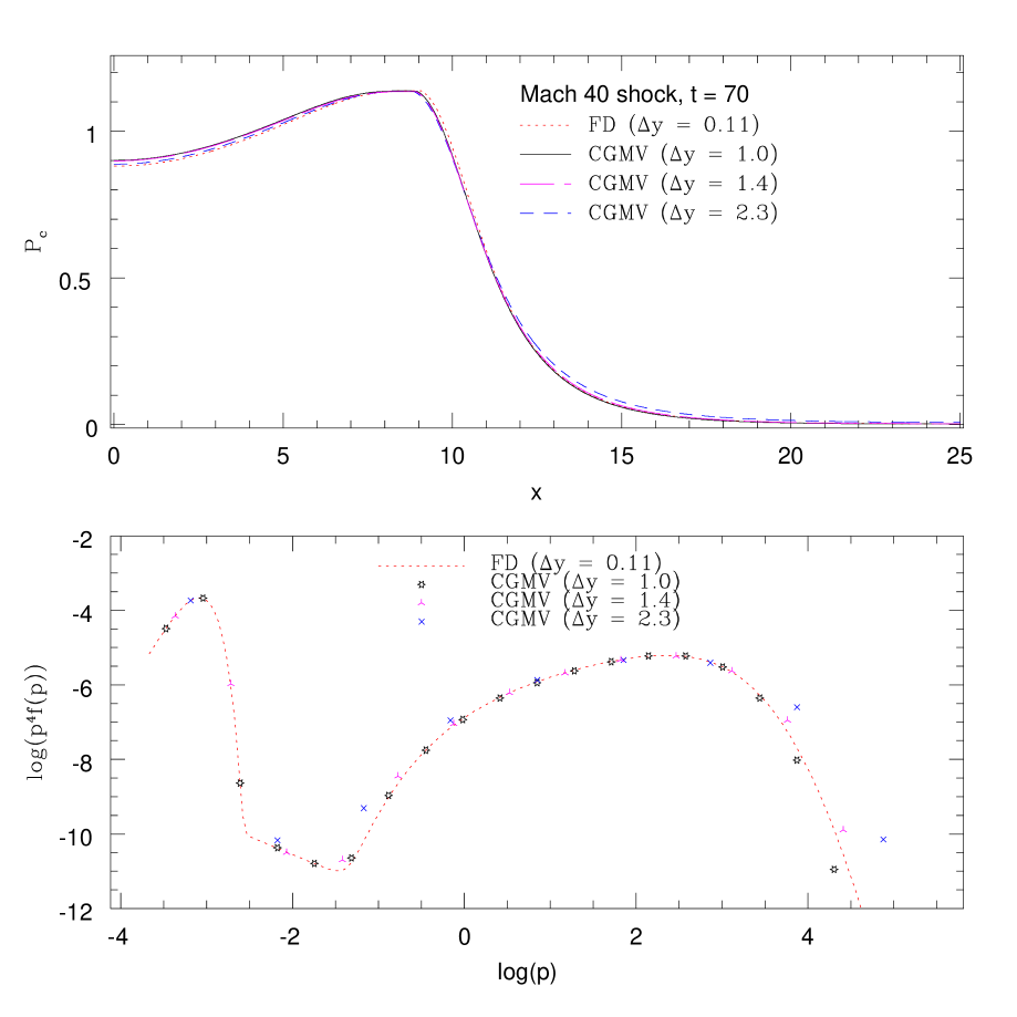
Since the efficiency of the CGMV method comes from its ability to cover the momentum range coarsely, it is important to evaluate how broad the momentum bins can be and still faithfully model the evolution of the shock. Fig. 3 illustrates convergence of the CGMV scheme with respect to momentum bin size, , at for the flow modeled in Fig. 2. The upper panel plots the spatial distributions, while the lower panel shows the particle momentum distributions at the gas subshock. For reference the corresponding FD solution () is shown by the dotted red curves. Solutions from the CGMV scheme are plotted for , and . Even the coarsest of the CGMV solutions is in basic agreement with the other CGMV solutions and with the FD solution. Fine details in the momentum distribution are naturally obscured as the CGMV bin size increases. The largest bins with span a decade in CR momentum (), but still capture the basic dynamical properties of the CRs correctly.
However, the quality of the CGMV solutions deteriorates for still larger momentum bins in these experiments, once the simple subgrid model for the momentum distribution becomes inadequate. As illustrated in the lower panel of Fig. 3 already momentum bins larger than roughly cannot closely follow sharper structures in the momentum distibution that develops at the ends of the CR distribution. That enhances upstream of the subshock, where the flow is both cold and strongly compressed as it approaches the subshock. When the errors become excessive, for , in this case, -induced overcompression in this region can cause the Riemann solver in our TVD code to perform poorly or even to fail in high Mach number flows. In general the largest allowed momentum bin size, should depend on the strongest curvature of the CR momentum distribution function as well as the degree of shock modification.
3.2 CRASH Tests
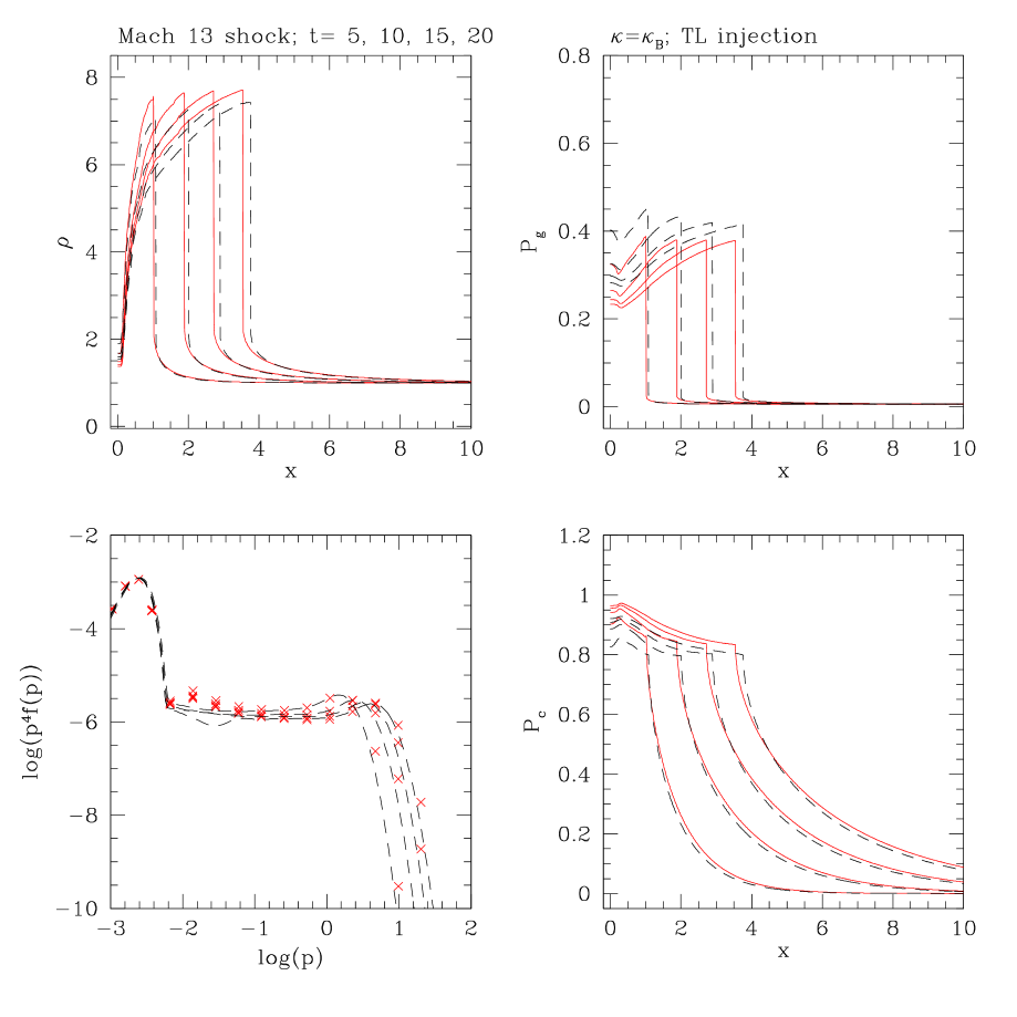
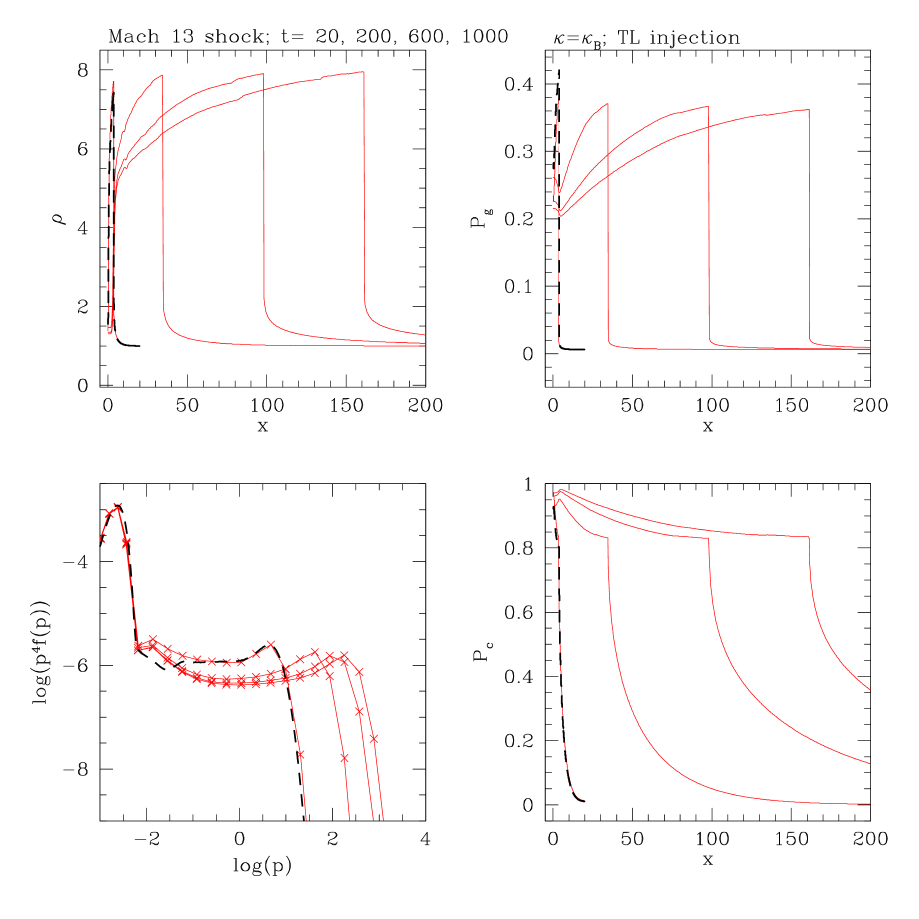
For a third test example we illustrate in Figs. 4 and 5 simulation results using the CRASH code with the TL injection model applied to a Mach 10 flow reflecting off the left computational boundary. The initial gas shock Mach number is approximately 13. As for the previous test, the upstream gas density and flow speed are set to unity, with upstream sound speed, , and . The time unit is defined accordingly. CR momenta are tracked over the range , where is the smallest momentum that can leak upstream (see equation 15).
In this case a Bohm-type diffusion model with , is adopted and the TL injection parameter, is used. The CRASH test was significantly more computationally demanding than the TVD-CR tests. Note first that in the CRASH simulation the value of , while in the previous examples shown in Figs. 1-3. Consequently, is about seven times greater in the current case, and the nominal physical scale of the precursor and its formation timescale are similarly lengthened. In addition, the stronger momentum dependence of Bohm diffusion coefficient means that the precursor width expands more strongly as increases. The associated time rate of increase in is, however, slower, so that the shock must evolve longer to reach a given . These factors substantially increase the size of the physical domain needed to reach a given .
Fig. 4 shows the early evolution of this CR-modified shock for as computed with both the FD and the CGMV methods. The spatial domain for this simulation is [0,20]. The base spatial grid included zones, giving . Since it is necessary to resolve structures near the subshock on scales of the diffusion length for freshly injected, suprathermal CRs, the AMR feature of the CRASH code is utilized. The FD simulation is carried out with 7 refined grid levels; four levels of refined grid are applied in the CGMV simulation. 240 momentum points ()are used in the FD simulation, while the CGMV simulation includes 20 momentum bins (). The time step for each refinement level, , is determined by a standard Courant condition, that is, . Although the Crank-Nicholson scheme is stable with an arbitrary time step, the diffusion convection equation is solved with the time step smaller than ) to maintain good accuracy in the momentum space advection (i.e., ). With , the required time step is smaller by a factor of three or so than the hydrodynamic time step in the FD simulation. Consequently, the FD diffusion convection solver is typically subcycled about 3 times with for each hydrodynamic time step. Because of the much larger , subcycling is not necessary in the CGMV simulation. That adds another relative economy to the CGMV calculation.
At the end of this simulation, , the modified shock structure is approaching a dynamical equilibrium in the sense that the postshock values of , and will not change much at later times. Since this shock is weaker than the Mach 40 shocks examined earlier modifications are more moderate. On the other hand, as expected from the stronger momentum dependence of , the shock precursor broadens much more quickly in the present case. The cutoff in the CR distribution has reached roughly by . Longer term evolution of this shock will be addressed below.
The agreement between the FD and CGMV solutions shown in Fig. 4 is good, although not as close as it was in the examples illustrated in Fig. 1 and Fig. 2. The more apparent distinctions between the two solutions in the present case come from effective differences in the application of the TL injection model with Bohm diffusion in FD and CGMV methods. Recall that the CGMV scheme applies the diffusion coefficients averaged across the momentum bins (see equations 10, 13). The Bohm diffusion model has a very steep momentum dependence for nonrelativistic particles; namely, . At low momenta where injection takes place the averaging increases the effective diffusion coefficient, and, thus, the leakage flux of suprathermal particles, leading to higher injection rate compared to the FD scheme for the same TL model parameters. Consequently, the distribution function in the second bin at is slightly higher in the CGMV scheme, as evident in Figs. 4-5. Note that is anchored on the tail of Maxwellian distribution. The CGMV solutions accordingly show slightly more efficient CR acceleration than the FD solutions at early times. In this test is about 5 % greater in the CGMV simulation at . Since the CGMV scheme can be implemented with nonuniform momentum bins, such differences could be reduced by making the momentum bins smaller at low momentum in instances where the details relating to the injection rate were important.
We show in Fig. 5 the evolution of this same shock extended to , as computed with the CGMV method. This simulation is computed on the domain [0,800], spanned by a base spatial grid of zones, giving . We also included 7 refined grid levels at the subshock, giving . This grid spacing is insufficient for convergence at the injection momentum, , so that the very early evolution is somewhat slower than in the simulations shown in Fig. 4. However, once shock modification becomes strong evolution becomes roughly self-similar, as pointed out previously [25]. The time asymptotic states do not depend sensitively on the early injection history. The self-similar behavior results with Bohm diffusion from a match between the upstream and downstream extensions of the CR population. One also sees from the form of the distribution function in Fig. 5 that the postshock gas temperature has stabilized, while the previously-explained concave form to the CR distribution is better developed than it was at earlier times.
This simulation illustrates nicely the relative efficiency of the CGMV scheme. The equivalent FD simulation would be very much more expensive, because this model requires a long execution time and a large spatial domain. With Bohm diffusion for ultrarelativistic CRs, so that the scale of the precursor, . At the same time the peak in the CR momentum distribution extends relatively slowly, with . The required spatial grid is, thus, 40 times longer than for the shorter simulation illustrated in Fig. 4. The simulated time interval in the extended simulation was 50 times longer. Together those increase the total computational time by a factor 2000. The FD calculation with to took about 2 CPU days on our fastest available processor, so the extended simulation would have been unrealistic using the FD method. The extended CGMV simulation, however, required only about 10 times the effort of the shorter FD simulation, clearly demonstrating the efficiency of the CGMV scheme. This speed-up is a result of combination of several factors: 20 times larger grid spacing, no need for subcycling for the diffusion convection solver, and, of course, a smaller number of momentum bins.
4 Conclusions
Detailed time dependent simulations of nonlinear CR shock evolution are very expensive if one allows for inclusion of arbitrary, self-consistent and possibly time dependent spatial diffusion, as well as various other momentum dependent transport processes. The principal computational cost in such calculations is typically the CR transport itself, and, in self-consistent calculations, the analogous transport of the MHD wave turbulence that mediates CR transport. Tracking these behaviors requires adding at least one physical dimension to the simulations compared to the associated hydrodynamical calculations, since the collisionless media involved are sensitive to the phase space configurations of the particles and waves. Particle kinetic equations (commonly the so-called diffusion convection equation) provide a straightforward approach to addressing this problem and can be coupled conveniently with hydrodynamical equations that track mass and bulk momentum and energy effectively.
Momentum derivatives of the CR distribution function in the diffusion convection equation are most frequently handled by finite differences. Although it is simple, that approach requires moderately fine resolution in momentum space. That is a primary reason that such calculations are costly. Here we introduce a new scheme to solve the diffusion convection equation based on finite volumes in momentum space with a momentum bin spacing as much as an order of magnitude larger than that of the usual finite difference scheme. We demonstrate that this Coarse Grained Momentum finite Volume ( CGMV) method can be used successfully to model the evolution of strong, CR-modified shocks at much lower computational cost than the finite difference approach. The computation efficiency is greatly increased, not only because the number of momentum bins is smaller, but also because the required spatial grid spacing is less demanding due to the coarse-grained averaging of the diffusion coefficient used in the CGMV method. In addition, larger momentum bin size can eliminate the need of subcycling of the diffusion convection solver that can be necessary in some instances using finite differences in momentum. Thus, the combination of the CGMV scheme with AMR techniques as developed in our CRASH code, for example, should allow more detailed modeling of the diffusive shock acceleration process with a strongly momentum dependent diffusion model such as Bohm diffusion, or self-consistent treatments of CR diffusion and wave turbulence transport.
Acknowledgments
TWJ is supported by NSF grant AST03-07600, by NASA grants NAG5-10774, NNG05GF57G and by the University of Minnesota Supercomputing Institute. HK was supported by KOSEF through the Astrophysical Research Center for the Structure and Evolution of Cosmos (ARCSEC).
References
- [1] Achterberg A. Astron. & Astrophys. 98 (1982) 195
- [2] Bell, A. R. M.N.R.A.S. 182 (1978) 147
- [3] Berezhko E.G., Yelshin V.K., & Ksenofontov L.T. Astroparticle Physics 2 (1994) 215
- [4] Berezhko E.G., Ksenofontov L.T., & Yelshin V.K. Nuclear Physics B 39a (1995) 171
- [5] Blasi, P., Astroparticle Physics 16 (2002) 429
- [6] Drury, L. O’C., & Völk, H. J., Astrophys. J. 248 (1981) 344
- [7] Drury, L. O’C. Rept. Prog. Phys. 46 (1983) 973
- [8] Drury, L. O’C., & Falle, S. A. E. G. M.N.R.A.S. 223 (1986) 353
- [9] Ellison, D. C. & Eichler, D. Astrophys. J. (1984) 691
- [10] Ellison, D. C., Möbius, E., & Paschmann, G. Astrophys. J. 352 (1990) 376
- [11] Ellison, D. C., Giacalone, J, Burgress D., & Schwartz, S. J. JGR 98 (1993) 21085
- [12] Falle, S. A. E. & Giddings, J. R. M.N.R.A.S. 225 (1987) 399
- [13] Frank, A., Jones, T. W. & Ryu, D., Astrophys. J. 441 (1995) 629
- [14] Giacalone, J., Burgess, D., Schwartz, S. J. & Ellison, D. C. Astrophs. J. 402 (1993) 550
- [15] Gieseler, U. D. J., Jones, T. W. & Kang, H. Astron. & Astrophys. 364 (2000) 911
- [16] Harten, A. J. Comp. Phys. 49 (1983) 357
- [17] Jones, T. W. Astrophys. J. 619 (1993) 619
- [18] Jones, T. W. Astrophys. J. Supplements 90 (1994) 969
- [19] Jones, T. W., Ryu, D. & Engel, A., Astrophys. J. 512 (1999) 105
- [20] Jun, B.-I. & Jones, T. W., Astrophys. J. 511 (1999) 774
- [21] Kang, H. & Jones, T. W., M.N.R.A.S. 249 (1991) 439
- [22] Kang, H. & Jones, T. W., Astrophys. J. 447 (1995) 944
- [23] Kang, H. & Jones, T. W., Astrophys. J. 476 (1997) 875
- [24] Kang, H., Jones, T. W., LeVeque, R. J., and Shyue, K. M. Astrophys. J. 550 (2001) 737
- [25] Kang, H., Jones, T. W., & Gieseler, U.D.J. Astrophys. J. 579 (2002) 337
- [26] Lagage, P. O. & Cesarsky, C. J. Astron. & Astrophys. 125 (1983) 249
- [27] LeVeque, R. J., and Shyue, K. M. SIAM J. Scien. Comput. 16 (1995) 348
- [28] Malkov, M.A. Astrophys. J. 485 (1997) 638
- [29] Malkov, M.A. Astrophys. J. 511 (1999) L53
- [30] Malkov M.A., and Völk H.J. Adv. Space Res. 21 (1998) 551
- [31] Malkov M.A., & Drury, L.O’C. Rep. Progr. Phys. 64 (2001) 429
- [32] Marcowith, A. & Kirk, J. G. Astron. & Astrophys. 347 (1999) 391
- [33] Miniati, F. Comp. Phys. Comm. 141 (2001) 17
- [34] Skilling, J., M.N.R.A.S., 223 (1975) 353
- [35] Scholar, M. Geophys Res Lett. 17 (1990) 11