Characteristic QSO Accretion Disk Temperatures from Spectroscopic Continuum Variability

Abstract

Using Sloan Digital Sky Survey (SDSS) quasar spectra taken at multiple epochs, we find that the composite flux density differences in the rest frame wavelength range 1300–6000Å  can be fit by a standard thermal accretion disk model where the accretion rate has changed from one epoch to the next (without considering additional continuum emission components). The fit to the composite residual has two free parameters: a normalizing constant and the average characteristic temperature $\bar{T}^{*}$. In turn the characteristic temperature is dependent on the ratio of the mass accretion rate to the square of the black hole mass. We therefore conclude that most of the UV/optical variability may be due to processes involving the disk, and thus that a significant fraction of the UV/optical spectrum may come directly from the disk.

1 Introduction

It has long been suspected that QSOs are powered by matter accreting from a disk onto a supermassive black hole (e.g., Lin & Papaloizou, 1996; Ulrich, Maraschi, & Urry, 1997; Mirabel & Rodríguez, 1999, and references therein). Also, it is observed that QSOs typically present a “flattened” UV/optical spectra or a “big blue bump” (e.g., Shields, 1978; Malkan & Sargent, 1982; Camenzind & Courvoisier, 1984; Elvis et al., 1994; Czerny et al., 2003). In turn, the big blue bump has generally been interpreted as thermal disk emission (e.g., Elvis et al., 1986; Laor & Netzer, 1989; Sanders et al., 1989; Fiore et al., 1995; Gu et al., 2001; Shalyapin et al., 2002). The standard model is a geometrically thin disk with local thermal emission based on conservation of energy and angular momentum (Shakura & Sunyaev, 1973). The integrated standard disk model continuum presents a “flattened” spectrum due to the contribution of different disk surface temperatures at different radii. Reasonable agreements are found with the standard disk model and the UV/optical continuum of QSOs (e.g., Malkan, 1983; Czerny & Elvis, 1987; Wandel & Petrosian, 1988; Sun & Malkan, 1989; Laor, 1990; Krolik et al., 1991; Natali et al., 1998).

However, accretion disk continuum fits to the UV/optical spectra of QSOs typically require additional components such as the extrapolation of the X-ray continuum into the UV/optical, the extrapolation of the infrared continuum, and the inclusion of a “small blue bump” component near 3000Å (e.g., Malkan, 1983; Czerny & Elvis, 1987; Wandel & Petrosian, 1988; Sun & Malkan, 1989; Laor, 1990). Also, host galaxy light can contaminate the QSO spectrum at optical and longer wavelengths.

In this work, we study the residual UV/optical continuum (continuum difference) of QSOs when they vary from a “faint” phase to a “bright” phase, rather than the continuum itself at either phase. Wilhite et al. (2005) found that the emission lines vary relatively weakly with respect to continuum variations; the residual flux density is dominated by continuum changes. By analyzing a composite residual spectrum we find that the average UV/optical flux density difference can be accounted for by a standard accretion disk that has changed its mass accretion rate. The composite residual is constructed from hundreds of objects observed by the Sloan Digital Sky Survey (SDSS) (Wilhite et al., 2005). This study of the residual flux assumes that the UV/optical variability is due to only the disk itself, thus no additional emission components are considered when analyzing the residual. The advantage of this approach is that non-variable emission sources that could contribute to the continuum do not contribute to the residual.

We are currently studying individual QSO spectra taken from the SDSS. If the continuum UV/optical variability in individual objects can also be accounted for by a standard accretion disk at rest frame wavelengths longer than Ly$\alpha$ 1215Å emission, then we may have a method to probe the inner disk region by analyzing the difference between EUV rest frame residual spectra and the standard disk model predictions. The strongest flux density for a disk under typical QSO parameters would occur in the EUV, this emission would be produced in the inner disk region. In turn, the strongest deviations of a real disk from the standard disk model are expected to occur in the inner disk region due to radiative transfer effects (including X-ray irradiation) (e.g., Hubeny et al., 2001) and departures of the gravitational force from the standard Newtonian $r^{-2}$ law (e.g., Frank, King & Raine, 1992; Krolik, 1999).

In §2 we briefly discuss the emission distribution from a standard disk and present general relationships. We present the form in which the average characteristic disk temperature $\bar{T}^{*}$ is calculated by analyzing the residual spectrum in §3. In §4 we apply the discussions of the previous two sections to a composite spectrum constructed from SDSS data. Summary and conclusions are presented in §5.

2 Standard Disk Model

2.1 General Comments

We assume in this paper that the QSO UV/optical continuum variability is solely due to accretion disks, and that the changes in the accretion disk are due to changes in the mass accretion rate. We will assume that the radial emission follows that of the standard disk model.

It is obvious that the standard disk model is an idealization, just as the assumption of blackbody emission is an idealization for the continuum of stellar spectra. However, we choose to apply the standard model in the continuum variability analysis for three reasons. First, the standard disk model includes much of the physics involved in accretion disks, such as gravity from a large central mass determining the average velocity fields in the disk, angular momentum transport, conversion of gravitational energy to radiative emission (where in the standard model it is assumed to be locally blackbody), and monotonic increase of temperature with decreasing radius (except at radii close to the inner disk radius). Local blackbody emission is a reasonable first approximation that accounts for the relatively “flat” continuum spectrum observed in systems where accretion disks are inferred.

Second, the radial emission distribution of the standard model is independent of the vertical disk structure and the details that generate viscosity within the disk; thus, in the study of continuum variability, the standard model can be reduced to the dependence on only two basic physical parameters, namely: the central black hole mass $M_{bh}$ and the disk mass accretion rate $\dot{M}_{accr}$.

Third, although more detailed and probably more realistic models that calculate the disk continuum have been developed since Shakura & Sunyaev (1973) (e.g., Czerny & Elvis, 1987; Wandel & Petrosian, 1988; Sun & Malkan, 1989; Laor, 1990; Ross, Fabian, & Mineshige, 1992; Colemann & Shields, 1993; Shields & Colemann, 1994; Störzer, Hauschildt, & Allard, 1994; Dörrer et al., 1996; Hubeny et al., 2000, 2001), they do not present significant differences with the continuum of the standard model at wavelengths greater than $\sim$ 3600Å, and present the strongest differences at wavelengths lower than $\sim$ 1300Å (see Fig. 13 in Hubeny et al., 2001). Therefore, since we are analyzing rest wavelength ranges above 1300Å, we do not expect the conclusions of this work to be significantly affected by applying the standard model rather than a more detailed one.

More detailed models clearly show, for example, that radiative transfer effects (that must be present) can generate significant changes in the disk continuum in the EUV. Therefore, if the analysis presented here continues to hold up for individual objects, then we may be able to study the emission contribution and structure of the inner disk region by analyzing the deviations in EUV variability between the standard model and actual observations.

2.2 Radial Emission Distribution

In the standard accretion disk model (Shakura & Sunyaev, 1973), the disk is assumed to be in a steady state and to be azimuthally symmetric. Shear stresses transport angular momentum outwards as the material of the gas spirals inwards. Conservation of angular momentum leads to the following expression

$$W2\pi r^{2}-\dot{M}_{accr}\omega r^{2}=C\,\,\,({\rm constant})\;\;\;\;,$$ (1)

where $r$ is the radius, $\dot{M}_{accr}$ is the mass accretion rate, $\omega$ is the corresponding angular velocity, and $W$ is defined by

$$W\equiv\int\limits_{-z_{o}}^{z_{o}}w_{r\phi}\,dz\;\;\;\;,$$ (2)

where $z_{o}$ is the half thickness of the disk and $w_{r\phi}$ is shear stress between adjacent layers. With the additional assumption that the shear stresses are negligible in the inner disk radius

$$W={\dot{M}_{accr}\over 2\pi r^{2}}(\omega r^{2}-\omega_{i}r_{i}^{2})\;\;\;\;,$$ (3)

where $\omega_{i}$ is the angular velocity at the inner disk radius $r_{i}$.

Taking into account the work done by shear stresses, and assuming that as the mass accretes inwards the gravitational energy lost is emitted locally

$$Q={1\over 4\pi r}\;{d\over dr}\left[\dot{M}_{accr}\left({\omega^{2}r^{2}\over 2}-{GM_{bh}\over r}\right)-W2\pi\omega r^{2}\right]\;\;\;\;,$$ (4)

where $Q$ is the radiated energy per area of the disk surface, $G$ is the gravitational constant, and $M_{bh}$ is the black hole mass. Assuming that the disk material follows Keplerian orbits, i.e., the mass of the disk is negligible compared to that of the black hole

$$\omega=\left({GM_{bh}\over r^{3}}\right)^{1/2}\;\;\;\;;$$ (5)

from equations (3) and (4) one finds

$$Q(r)={3\dot{M}_{accr}GM_{bh}\over 8\pi r_{i}^{3}}\left(r_{i}\over r\right)^{3}\left[1-\left({r_{i}\over r}\right)^{1/2}\right]\;\;\;\;.$$ (6)

The function $Q(r)$ [eq. (6)] was originally derived by Shakura & Sunyaev (1973) for binary systems with an accretion disk rotating about a black hole.

Further, assuming that the disk is emitting locally as a blackbody, the radial temperature distribution of the disk will be given by

$$T(r)=\left\{{3\dot{M}_{accr}GM_{bh}\over 8\pi r_{i}^{3}\sigma_{s}}\right\}^{1/4}\left\{\left(r_{i}\over r\right)^{3}\left[1-\left({r_{i}\over r}\right)^{1/2}\right]\right\}^{1/4}\;\;\;\;,$$ (7)

where $\sigma_{s}$ is the Stefan-Boltzmann constant.

Defining the characteristic disk temperature $T^{*}$

$$T^{*}\equiv\left\{{3\dot{M}_{accr}GM_{bh}\over 8\pi r_{i}^{3}\sigma_{s}}\right\}^{1/4}\;\;\;\;,$$ (8)

the expression of the radial temperature distribution becomes

$$T(r)=T^{*}\left\{\left(r_{i}\over r\right)^{3}\left[1-\left({r_{i}\over r}\right)^{1/2}\right]\right\}^{1/4}\;\;\;\;.$$ (9)

To further simplify mathematical expressions, we define the function $t(x)$

$$t(x)\equiv\left\{x^{-3}\,\left[1-x^{-1/2}\right]\right\}^{1/4}\;\;\;\;,$$ (10)

thus

$$T(r)=T^{*}\,t(r/r_{i})\;\;\;\;.$$ (11)

Since $r_{i}$ is the inner disk radius, $r\geq r_{i}$. It follows that

$$\max(t(r/r_{i}))=t(7^{2}/6^{2})={6^{3/2}\over 7^{7/4}}\approx 0.488\;\;\;\;.$$ (12)

Therefore the maximum temperature of a standard disk $T_{max}$ is given by

$$T_{max}\equiv\max(T(r))={6^{3/2}\over 7^{7/4}}\,T^{*}\approx 0.488\,T^{*}\;\;\;\;;$$ (13)

that is, the maximum surface temperature of a standard disk $T_{max}$ is approximately one-half of the characteristic temperature $T^{*}$.

The total disk luminosity $L_{disk}$ is given by

$$L_{disk}=\int_{r_{i}}^{r_{f}}4\pi r\,Q(r)\,dr\;\;\;\;,$$ (14)

where $r_{f}$ is the outer disk radius. Thus, substituting equation (6) into equation (14),

$$L_{disk}={\dot{M}_{accr}GM_{bh}\over 2r_{i}}\left\{1-{3r_{i}\over r_{f}}\left[1-{2\over 3}\left({r_{i}\over r_{f}}\right)^{1/2}\right]\right\}\;\;\;\;.$$ (15)

Since we are assuming local blackbody emission, the luminosity density $F_{\lambda}$ of the disk is given by

$$F_{\lambda}=\int_{r_{i}}^{r_{f}}\pi\,B_{\lambda}(T(r))\,4\pi r\,dr\;\;\;\;,$$ (16)

where $B_{\lambda}(T)$ is the blackbody intensity at temperature $T$. That is

$$F_{\lambda}=\int\displaylimits_{r_{i}}^{r_{f}}{\pi\,{{2hc^{2}\over\lambda^{5}}\over\exp\left(hc\over\lambda\,kT^{*}t(r/r_{i})\right)-1}\,4\pi r\,dr}\;\;\;\;,$$ (17)

where $h$ is Plank’s constant, $c$ is the speed of light, and $k$ is Boltzmann’s constant. Thus it follows that

$$L_{disk}=\int_{0}^{\infty}F_{\lambda}\,d\lambda\;\;\;\;.$$ (18)

The radial emission distribution of a standard disk [eqs. (6), (8), (10), and (11)] and its luminosity density [eqs. (17) and (10)] are dependent on only four physical parameters: the black hole mass $M_{bh}$, the mass accretion rate $\dot{M}_{accr}$, the innermost radius of the disk $r_{i}$, and the outermost radius of the disk $r_{f}$.

The nine assumptions used to derive the expressions for the radial emission distribution of a standard disk are: 1) the disk is steady; 2) the disk is azimuthally symmetric; 3) the gravitational field is Newtonian; 4) the mass of the disk is negligible compared to that of the black hole; 5) the mass within the disk follows Keplerian orbits; 6) conservation of angular momentum holds as shear stresses cause the disk mass to spiral inwards; 7) the shear stress in the disk at the innermost radius is zero; 8) conservation of energy holds as the loss of gravitational energy is converted into radiation; and 9) the disk surface emission is locally blackbody.

2.3 Additional Assumptions

We will apply two additional assumptions that reduce the dependence of the disk luminosity density to only two parameters: black hole mass $M_{bh}$ and mass accretion rate $\dot{M}_{accr}$.

First, we shall assume that the outer disk radius $r_{f}$ is much larger than the inner disk radius $r_{i}$:

$$r_{f}\gg r_{i}\;\;\;\;.$$ (19)

This assumption not only eliminates a free parameter, but it is justified since most of the UV/optical emission is coming from the inner disk region [eq. (9)]. Beyond a certain radius the disk contribution to the UV/optical continuum is negligible, even if the disk were to actually extend to infinity.

After making this assumption, the expression for disk luminosity [eq. (15)] becomes

$$L_{disk}={\dot{M}_{accr}GM_{bh}\over 2\,r_{i}}\;\;\;\;,$$ (20)

and the luminosity density [eq. (17)] is now given by

$$F_{\lambda}=\int\displaylimits_{r_{i}}^{\infty}{\pi\,{{2hc^{2}\over\lambda^{5}}\over\exp\left(hc\over\lambda\,kT^{*}t(r/r_{i})\right)-1}\,4\pi r\,dr}\;\;\;\;.$$ (21)

Defining

$$s\equiv{r\over r_{i}}\;\;\;\;,$$ (22)

and rewriting the integral in equation (21) in terms of variable $s$, the expression for the luminosity density becomes

$$F_{\lambda}=r_{i}^{2}\;\int\displaylimits_{1}^{\infty}{\pi\,{{2hc^{2}\over\lambda^{5}}\over\exp\left(hc\over\lambda\,kT^{*}t(s)\right)-1}\,4\pi s\,ds}\;\;\;\;.$$ (23)

The shape of the luminosity density (i.e., the dependence of the luminosity density on wavelength within a multiplying constant) depends only on one physical parameter, the characteristic temperature $T^{*}$ [eq. (8)].

Since a real disk will have a finite outer radius, the actual shape of the disk luminosity density, beyond a certain wavelength, will depend strongly on the exact position of the outer radius; however, if the disk is of sufficient size, the strong dependence on the outer disk radius will occur at infrared wavelengths and beyond. While in the UV/optical continuum, the difference between taking into account the actual outer disk radius with respect to assuming an infinite disk would be indistinguishable.

Second, we shall also assume, as was done by Shakura & Sunyaev (1973), and as is standard in the literature, that the innermost disk radius is given by the last stable circular orbit as determined by General Relativity (GR) under a Schwarzschild metric:

$$r_{i}={6\,GM_{bh}\over c^{2}}\;\;\;\;.$$ (24)

The expression for disk luminosity [eq. (20)] now becomes

$$L_{disk}={1\over 12}\;\dot{M}_{accr}c^{2}\;\;\;\;.$$ (25)

In other words, if the outer radius extends to infinity, and the standard model’s expression for the inner disk radius [eq. (24)] is correct, the efficiency of a standard disk is $1\over 12$. The expression of $L_{disk}$ now depends on only one physical parameter, the mass accretion rate $\dot{M}_{accr}$. Deviations of the inner disk radius from the standard expression [eq. (24)] may generate corrections to equation (25). In particular, if one were to assume the innermost disk radius $r_{i}$ to be the last stable direct circular orbit as calculated in GR under a Kerr metric (rather than a Schwarzschild metric, e.g. Bardeen, Press, & Teukolsky, 1972), one would find smaller values for $r_{i}$ (for a discussion on GR corrections under a Kerr metric for the radial emission distribution of a steady accretion disk see Novikov & Thorne, 1973; Page & Thorne, 1974).

The expression for the characteristic temperature [eq. (8)] now becomes

$$T^{*}\equiv\left\{{\dot{M}_{accr}c^{6}\over 576\,\pi\,G^{2}M_{bh}^{2}\sigma_{s}}\right\}^{1/4}\;\;\;\;.$$ (26)

Substituting equation (24) into equation (23), the expression for the luminosity density becomes:

$$F_{\lambda}=\left(6G\over c^{2}\right)^{2}\;M_{bh}^{2}\;\int\displaylimits_{1}^{\infty}{\pi\,{{2hc^{2}\over\lambda^{5}}\over\exp\left(hc\over\lambda\,kT^{*}t(s)\right)-1}\,4\pi s\,ds}\;\;\;\;.$$ (27)

Thus, we find the explicit expression for luminosity density that we apply here [eq. (27); eq. (10)]. From equation (27), it can be seen that the disk continuum shape depends on only one physical parameter, the characteristic temperature $T^{*}$.

2.4 Qualitative Comparison with Observations

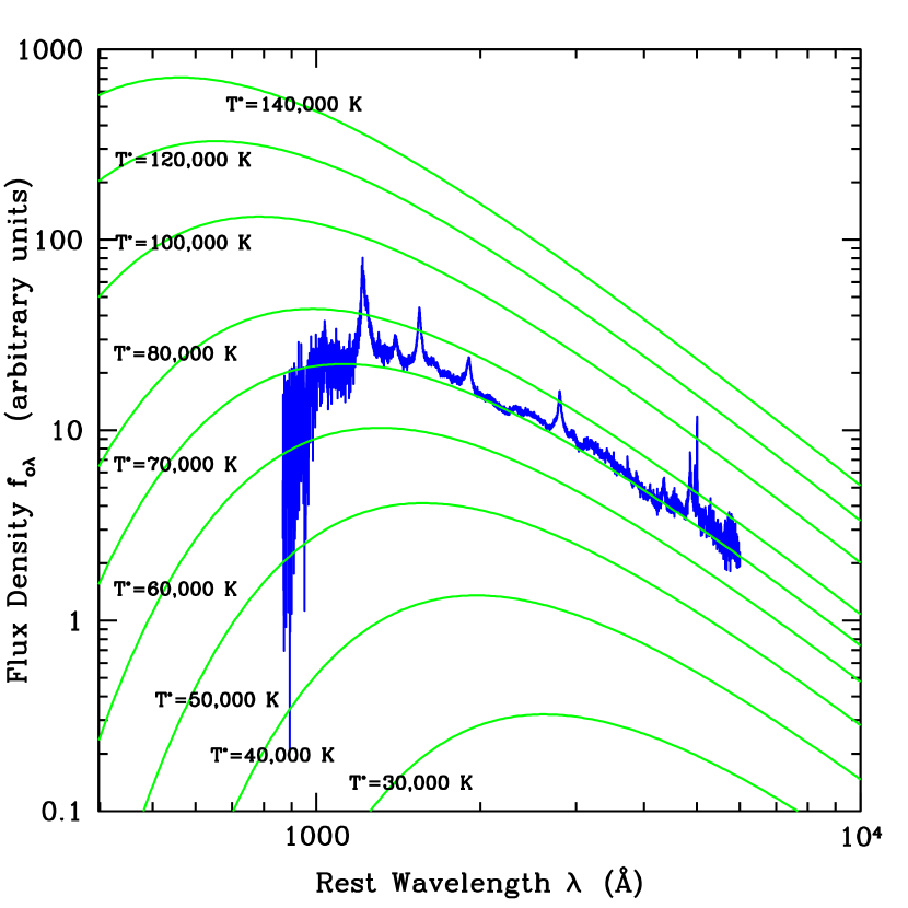
Figure 1: Flux density of an SDSS QSO composite spectrum (blue) in arbitrary units vs. rest wavelength in Å, superimposed with the luminosity density of a standard disk with different characteristic temperatures $T^{*}$ (green) in arbitrary units. The disk mass accretion rate $\dot{M}_{accr}$ is proportional to $(T^{*})^{4}$ [eq. (26)]. This plot illustrates that that the UV/optical continuum of QSOs is qualitatively consistent with thermal emission from an accretion disk. Also, different $T^{*}$ values lead to changes in the shape of the disk continuum spectrum.

As discussed in the Introduction, different authors have noted that the “flattened” UV/optical spectra observed in QSOs is qualitatively consistent with disk models. To illustrate this point, we show in Figure 1 the luminosity density calculated using equation (27) for different disk mass accretion rates superimposed with a QSO composite constructed from SDSS data (Wilhite et al., 2005). In Figure 1, it can be seen that changes in the mass accretion rate $\dot{M}_{accr}$ produce changes in the form of the disk continuum spectrum. Therefore, residual spectra (i.e., the difference between two spectra observed at different epochs) can be used to make comparisons with disk models, as we do here.

The majority of QSOs/AGN present continuum variability on the order of 10% on timescales of months to years (Sirola et al., 1998; Vanden Berk et al., 2004). These timescales are roughly consistent with estimated sound-speed timescales of the accretion disks in QSOs/AGN. Sound-speed timescales measure the time it takes a density/pressure perturbation (i.e., a sound wave) to travel over a significant portion of the disk. In turn, the total pressure is equal to the sum of gas pressure and radiation pressure; for the standard disk within typical QSO/AGN parameters, the disk height in the inner disk region is determined by radiation pressure (rather than gas pressure). This implies that if one estimates the sound speed solely taking into account gas pressure (i.e., taking radiation pressure to be zero), one significantly underestimates the sound speed in the inner disk region, and thus significantly overestimates the sound-speed timescales.

Two additional characteristic disk timescales that should be mentioned at this point (see e.g. Pringle, 1981) are the thermal timescale and the viscous or inflow timescale (for estimates of different disk timescales for QSO/AGN parameters, see e.g. Webb & Malkan, 2000). The thermal timescale is the ratio of the disk thermal content to its heating rate for a given patch of disk (Krolik, 1999). The viscous or inflow timescale is the time it takes a disk particle to travel a significant radial portion of the disk as it spirals inwards. The viscous or inflow timescale at a given radius may be estimated by the ratio of the given radius to the corresponding radial flow velocity, and can be thought of as the accretion timescale (Krolik, 1999). Also, it should be noted that spectroscopic changes occur across the entire spectrum whenever any part of the disk emission changes. So, even if the propagation speed were relatively slow, since the inner disk dominates the spectrum, and since the inner disk would change most rapidly, changes across the spectrum would still occur on relatively short timescales.

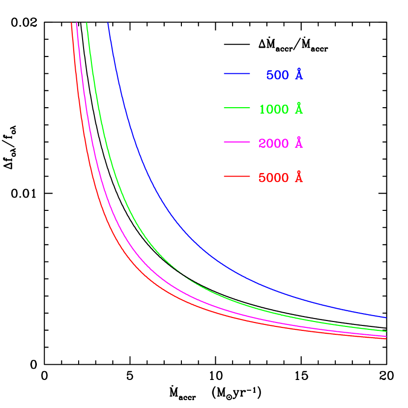
Figure 2: Relative change in flux density of a standard disk vs. mass accretion rate for different wavelengths. The value of black hole mass used is $M_{bh}=10^{9}\,M_{\sun}$. The change in mass accretion rate is assumed constant ($\Delta\dot{M}_{accr}=0.04\,M_{\sun}\,{\rm yr}^{-1}$). This figure shows that, within typical QSO parameters, the continuum spectrum of a standard disk becomes bluer as its mass accretion rate increases [or equivalently, as its luminosity increases; see eq. (25)]. This is consistent with observations of UV/optical variability in QSOs, in that, as discussed in the text, the QSO UV/optical continuum typically becomes bluer as it becomes brighter.

Figure 2 shows the relative change in flux density of a standard disk vs. mass accretion rate for different wavelengths. The value of black hole mass used is $M_{bh}=10^{9}\,M_{\sun}$. The change in mass accretion rate is assumed constant ($\Delta\dot{M}_{accr}=0.04\,M_{\sun}\,{\rm yr}^{-1}$). Figure 2 shows that, within typical QSO parameters, the continuum spectrum of a standard disk becomes bluer as its mass accretion rate increases [or equivalently, as its luminosity increases; see eq. (25)]. This is qualitatively consistent with observations that show that the optical/UV continua of QSOs are generally bluer in more luminous phases (e.g., Cutri et al., 1985; Edelson, Krolik, & Pike, 1990; Kinney et al., 1991; Paltani & Courvoisier, 1994; Webb & Malkan, 2000; Vanden Berk et al., 2004; Wilhite et al., 2005).

3 Determination of $\bar{T}^{*}$ from the Residual Spectrum

3.1 General Comments

In performing fits to the residual spectrum, we assume that the shape of the disk flux continuum is isotropic (foreshortening effects will introduce a viewing angle dependence to the observed disk flux, but independent of wavelength), and thus the observed disk flux would be equal to the luminosity density up to a normalizing constant. Relativistic effects will introduce dependence of the continuum shape on viewing angle (e.g., special relativistic beaming and GR light bending). Radiative transfer effects (e.g., limb darkening) will also introduce dependence of the continuum shape on viewing angle; however, disk atmosphere models suggest that for wavelength ranges above $\sim$ 3600Å significant changes in the continuum shape will occur only at high viewing angles (close to edge-on). The strongest changes for wavelengths between $\sim$ 1300 and $\sim$ 3600Å will also occur at high viewing angles (see Fig. 12 in Hubeny et al., 2000), and that would include only a fraction of objects assuming a random disk orientation in the QSO population.

3.2 Determination of the Average Characteristic Disk Temperature $\bar{T}^{*}$

To simplify the expressions, we define

$$g_{\lambda}(T^{*})\equiv\int\displaylimits_{1}^{\infty}{\pi\,{{2hc^{2}\over\lambda^{5}}\over\exp\left(hc\over\lambda\,kT^{*}t(s)\right)-1}\,4\pi s\,ds}\;\;\;\;.$$ (28)

The observed disk flux density $f_{o\lambda}$ will be proportional to the disk luminosity density [eq. (27)]. Therefore,

$$f_{o\lambda}=c_{o}\;g_{\lambda}(T^{*})\;\;\;\;,$$ (29)

where $c_{o}$ is a constant that depends on the black hole mass [see eq. (27)], the object’s cosmological distance, and the disk viewing angle (through foreshortening).

In this work, we assume that between the two epochs, the disk evolves from one steady state to another steady state with a change in mass accretion rate $\Delta\dot{M}_{accr}$. Since the black hole mass would not change significantly on the timescales considered here, it follows that the normalizing factor $c_{o}$ remains constant, but the characteristic disk temperature $T^{*}$ will vary [eq. (26)]. Therefore, the residual spectrum $\Delta f_{o\lambda}$ is given by

$$\Delta f_{o\lambda}=f_{2o\lambda}-f_{1o\lambda}=c_{o}\;g_{\lambda}(T^{*}_{2})-c_{o}\;g_{\lambda}(T^{*}_{1})=c_{o}\;\left(g_{\lambda}(T^{*}_{2})-g_{\lambda}(T^{*}_{1})\right)$$ (30)

where the subindexes $1$ and $2$ correspond to each epoch.

Considering a Taylor series about the average characteristic temperature

$$\bar{T}^{*}\equiv{1\over 2}\,(T^{*}_{2}+T^{*}_{1})\;\;\;\;,$$ (31)

and defining

$$\Delta T^{*}\equiv T^{*}_{2}-T^{*}_{1}\;\;\;\;,$$ (32)

we have

$$g_{\lambda}(T^{*}_{2})=g_{\lambda}(\bar{T}^{*})+\left(\Delta T^{*}\over 2\right)\left.\partial g_{\lambda}\over\partial T^{*}\right|_{\bar{T}^{*}}+{1\over 2}\,\left(\Delta T^{*}\over 2\right)^{2}\left.\partial^{2}g_{\lambda}\over\partial T^{*2}\right|_{\bar{T}^{*}}+{1\over 6}\,\left(\Delta T^{*}\over 2\right)^{3}\left.\partial^{3}g_{\lambda}\over\partial T^{*3}\right|_{\bar{T}^{*}}+\cdots\;\;\;\;,$$ (33)

and

$$g_{\lambda}(T^{*}_{1})=g_{\lambda}(\bar{T}^{*})-\left(\Delta T^{*}\over 2\right)\left.\partial g_{\lambda}\over\partial T^{*}\right|_{\bar{T}^{*}}+{1\over 2}\,\left(\Delta T^{*}\over 2\right)^{2}\left.\partial^{2}g_{\lambda}\over\partial T^{*2}\right|_{\bar{T}^{*}}-{1\over 6}\,\left(\Delta T^{*}\over 2\right)^{3}\left.\partial^{3}g_{\lambda}\over\partial T^{*3}\right|_{\bar{T}^{*}}+\cdots\;\;\;\;.$$ (34)

It follows that

$$g_{\lambda}(T^{*}_{2})-g_{\lambda}(T^{*}_{1})=\Delta T^{*}\,\left.\partial g_{\lambda}\over\partial T^{*}\right|_{\bar{T}^{*}}+{1\over 3}\,\left(\Delta T^{*}\over 2\right)^{3}\left.\partial^{3}g_{\lambda}\over\partial T^{*3}\right|_{\bar{T}^{*}}+\cdots\;\;\;\;.$$ (35)

Therefore, considering equation (30), the residual spectrum $\Delta f_{o\lambda}$ is given by

$$\Delta f_{o\lambda}=c_{o}\,\Delta T^{*}\,\left.\partial g_{\lambda}\over\partial T^{*}\right|_{\bar{T}^{*}}+{c_{o}\over 3}\,\left(\Delta T^{*}\over 2\right)^{3}\left.\partial^{3}g_{\lambda}\over\partial T^{*3}\right|_{\bar{T}^{*}}+\cdots\;\;\;\;.$$ (36)

In this work, to simplify the analysis, we introduce the following approximation

$$\Delta f_{o\lambda}\approx c_{o}\,\Delta T^{*}\,\left.\partial g_{\lambda}\over\partial T^{*}\right|_{\bar{T}^{*}}\;\;\;\;.$$ (37)

The function $g_{\lambda}$ [equation (28)] depends on only one independent physical parameter, the characteristic temperature $T^{*}$. Therefore, the process of fitting the residual spectra is reduced to the determination of two parameters: the product $c_{o}\,\Delta T^{*}$ and the average characteristic temperature $\bar{T}^{*}$.

We determine these two parameters by the standard method of maximum likelihood under the assumption of Gaussian flux density error distributions. That is, we determine the values of the two free parameters, “$c_{o}\,\Delta T^{*}$” and “$\bar{T}^{*}$,” that minimize

$$\chi^{2}\equiv\sum_{i}{1\over\sigma_{i}^{2}}\,\left(\Delta f_{o\lambda i}-[c_{o}\,\Delta T^{*}]\,\left.\partial g_{\lambda i}\over\partial T^{*}\right|_{\bar{T}^{*}}\right)^{2}\;\;\;\;,$$ (38)

where $\sigma_{i}$ is the error on the measurement of flux density variation at wavelength $\lambda_{i}$. The standard deviation on the values of each of the two free parameters is calculated assuming, once again, standard Gaussian distributions.

3.3 Testing the Method Against “Simulated” Data

In order to test the ability of the method described in §3.2 to determine correct values of $\bar{T}^{*}$ , we shall apply it to “simulated” data in which the exact value of $\bar{T}^{*}$ is previously known.

For the test data, we have fixed the value $\bar{T}^{*}=70,000\,{\rm K}$ (which corresponds to typical QSO parameters: $M_{bh}=10^{9}M_{\sun}$, $\dot{M}_{accr}\approx 1\;M_{\sun}\,{\rm yr^{-1}}$), and have varied the value of $\Delta T^{*}$ for the assumed constant black hole mass of $M_{bh}=10^{9}M_{\sun}$. We have also assumed an error of 5% on measurement of flux density at all wavelengths for both the “bright” and the “faint” epochs.

That is, we have calculated the luminosity density for $T^{*}_{2}=\bar{T}^{*}+\Delta T^{*}/2$ from equation (27) for $\bar{T}^{*}=70,000\,{\rm K}$, for the aforementioned value of black hole mass, for a discrete number of wavelengths between 1300Å and 6000Å, and taken these to be the measured data points for the bright phase with a measurement error of 5% on all points. Equivalently, we have also calculated the luminosity density for $T^{*}_{1}=\bar{T}^{*}-\Delta T^{*}/2$ from equation (27) and taken these values to be the measured data points for the faint phase. The specific values used for the wavelengths $\lambda_{i}$ are taken to be same as those obtained through the construction of the SDSS composite spectra that is studied in §4.

In Figure 3, we show the estimated value $\bar{T}^{*}$ vs. the variation in temperature $\Delta T^{*}$. For the above parameters, accurate values for $\bar{T}^{*}$ are obtained for variations in temperature of up to $\Delta T\approx 15,000\,{\rm K}$. That is, the method estimates accurate values for $\bar{T}^{*}$ (for the parameters used here) for changes in mass accretion rate $\dot{M}_{accr}$ of up to approximately a factor of two [see eq. (26)]. The reason that the characteristic temperature $\bar{T}^{*}$ becomes overestimated for larger variations in temperature $\Delta T^{*}$ (see Figure 3), is that the third and greater order terms of equation (36) are no longer negligible.

In Figure 4, we show the standard deviation of the estimated value of $\bar{T}^{*}$, $\sigma_{\bar{T}^{*}}$ vs. the variation in temperature $\Delta T^{*}$. For the above physical parameters, the standard deviation $\sigma_{\bar{T}^{*}}$ is less than $15,000\,{\rm K}$ for values of $\Delta T^{*}$ greater than $\approx 250\,{\rm K}$. The reason that $\sigma_{\bar{T}^{*}}$ becomes significantly large (i.e., comparable to the value of $\bar{T}^{*}$) at very low temperature variations $\Delta T^{*}$, is that errors on the flux measurements of the bright and faint phases become larger than the residual flux density.

Thus, we have shown that for a disk characteristic temperature of $70,000\,{\rm K}$, if the UV/optical variability in QSOs is due to changes in mass accretion rate $\dot{M}_{accr}$, then the method described in §3.2 will be capable of accurately and effectively constraining the average disk characteristic temperature $\bar{T}^{*}$, as long as the temperature variation $\Delta T^{*}$ is greater than $\approx 250\,{\rm K}$ and the changes in mass accretion rate $\dot{M}_{accr}$ are not significantly greater than about a factor of two.

4 Application to SDSS Composite Spectra

4.1 Construction of the Composite Residual Spectrum

The systematic construction of the composite residual spectrum from over 300 QSOs taken from the SDSS is discussed in detail in a separate paper (Wilhite et al., 2005). To avoid redundancy, we shall present here only a brief discussion of the construction of the composite, and focus rather on analyzing the composite residual within the assumption that it is generated by a change in mass accretion rate of a standard disk that evolves from one steady state to another, applying the methods discussed above.

The SDSS (see York et al., 2000; Stoughton et al., 2002, and references therein for a technical summary) is producing a large homogeneous sample of spectroscopically observed QSOs (Schneider et al., 2003). The QSOs are targeted (Blanton et al., 2003) according to the algorithm described by Richards et al. (2002) from photometric data in the SDSS imaging survey (Fukugita et al., 1996; Gunn et al., 1998; Hogg et al., 2001; Smith et al., 2002; Pier et al., 2003; Ivezic et al., 2004). Most of the QSOs used by Wilhite et al. (2005) are identified in the third SDSS data release (Abazajian et al., 2005). QSOs that were spectroscopically observed at least twice by the SDSS (see Figure 5 for a rest frame time lag histogram of the sample) were searched for clear evidence of variability in the observer frame optical (UV/optical QSO rest frame). Stars observed simultaneously with the QSOs were used to calibrate the observed fluxes (under the assumption that the stellar fluxes are constant), and to systematically establish the maximum variation in flux density measurements that could be attributed to experimental noise.

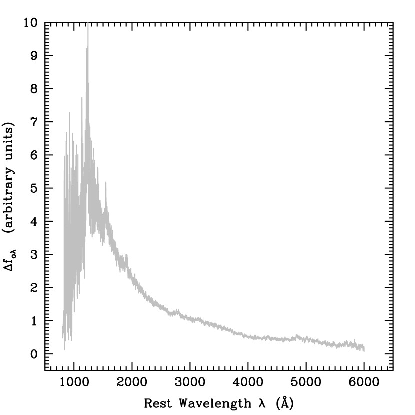
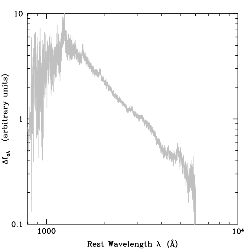
Figure 6: (Left) Composite QSO residual spectrum derived from SDSS data. (Right) Same plot in log-log scale. Details on the construction of the composite are presented in a separate paper (Wilhite et al., 2005). The flux density of the residual spectrum tends to become larger at lower wavelengths. Although the strength of the emission lines is significantly reduced in the residual spectra, with respect to corresponding line strengths in the spectra of either the bright or faint phases (e.g., see Figure 1), they are still detectable.

A residual spectrum was calculated for each of the QSOs that were identified to have clearly presented a variation in its UV/optical rest frame continuum. The individual rest frame residual spectra were scaled to unity at a predefined wavelength (3060Å). The composite residual (Figure 6) was then constructed by averaging the individually scaled residual spectra.

4.2 Fitting the Residual Spectrum

Following the methods discussed in §3.2, we have fit the SDSS composite residual spectrum discussed in §4.1. As discussed in §3.2, the two free parameters of the fit are a constant scaling factor and the average disk characteristic temperature $\bar{T}^{*}$. As discussed by Wilhite et al. (2005), the strength of the emission line components in the residual are significantly reduced with respect to the line strengths in the spectra of either the bright or faint phases; this point is illustrated by comparing Figures 1 and 6. That is, relative to the continuum variations, the emission lines vary relatively weakly. However, residual features at the locations of some major emission lines are visible in the composite difference spectrum.

We calculate several different fits to the residual spectrum by using the whole data spectrum (800-6000Å), by excluding wavelengths below 912Å (i.e., below the Lyman limit), by excluding wavelengths below 1300Å (to exclude flux contributions from the Ly$\alpha$ 1215Å line and to avoid the Ly$\alpha$ forest absorption), and by excluding the contribution of other strong emission lines. The results are presented in Table 1. The first column gives the wavelength ranges used for the fits, the second column lists strong emission lines whose flux contributions are excluded from the fits (due to the wavelength ranges of the first column), the third column gives the derived average characteristic temperatures $\bar{T}^{*}$, the fourth column gives the derived uncertainties (2$\,\sigma$) on $\bar{T}^{*}$ (calculated under the standard assumption of Gaussian distributions), and the fifth column gives the reduced chi-square values $\chi^{2}/n$ (where $n$ is the number of degrees of freedom [# of data points - # of free parameters]).

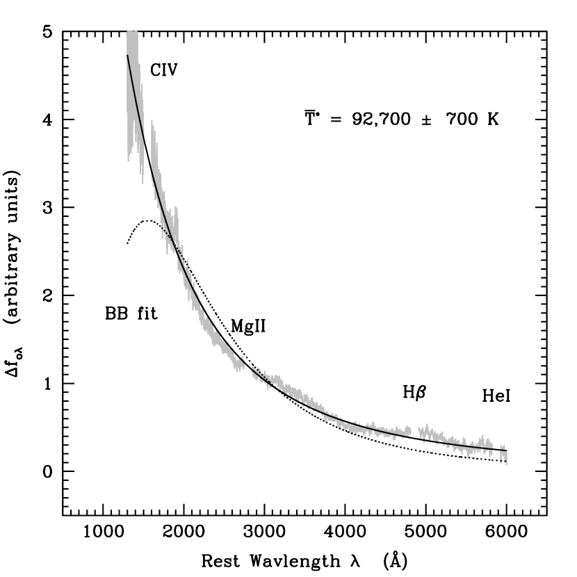
Figure 7: Composite QSO residual spectra derived from SDSS data, excluding wavelengths lower than 1300 Å  and excluding wavelengths associated with the four emission lines indicated, superimposed with the fit of a disk (solid curve) that has changed its mass accretion rate $\dot{M}_{accr}$. The average characteristic temperature of the fit is $\bar{T}^{*}=92,700\,{\rm K}$ (see last row of Table 1). The maximum disk surface temperature $T_{max}$ is approximately one-half of the characteristic temperature $T^{*}$ (see §2.2). In addition, the best blackbody fit (dotted curve; $T_{BB}=15,500{\rm K}$) to the composite residual is also shown.

In Figure 7, we present the composite QSO residual spectra derived from SDSS data excluding wavelengths lower than 1300Å, and excluding wavelengths associated with the four emission lines indicated in the second column of the last row of Table 1, superimposed with the fit of a standard disk that has changed its mass accretion rate $\dot{M}_{accr}$. The average characteristic temperature of the fit is $\bar{T}^{*}=92,700\,{\rm K}\pm 700\,{\rm K}$ and the value for the reduced chi-square of the fit is $\chi^{2}/n=2.993$ (see the last row of Table 1). Figure 7 shows that the composite residual spectrum is quantatively consistent with the assumption that the residual is caused by the change of mass accretion rate $\dot{M}_{accr}$ in a standard disk.

The best fit to the residual spectrum for a single-temperature blackbody is also shown in Figure 7. The blackbody fit with a temperature of $15,500$K is clearly quite poor. Models for which the difference spectrum might reasonably be described by a single blackbody, such as individual supernova explosions or localized hot spots, are not supported by the composite residual spectrum.

Almost all the data used here are different subsets of wavelengths above the Lyman limit (912Å) of the QSO rest frame (Table 1). Below these wavelengths it is likely that deviations between the observations and the standard disk model will occur for several reasons. First, as discussed in the Introduction, deviations of a real disk from the standard model are expected below the Lyman limit due to radiative transfer effects and due to the departure of the gravitational force from the standard Newtonian form in the inner disk region. Second, for higher redshifts QSOs, it is more likely that neutral hydrogen intervening systems will produce significant absorption (Ly$\alpha$ forest) “occulting” of the disk continuum at wavelengths lower than the Ly$\alpha$ 1215Å. A third reason is that other possibly variable components, such as a Compton upscattering component extending from X-ray wavelengths, which do not originate directly from the disk, will be important.

The average characteristic temperature that we derive from the composite residual spectra is thus independent of the continuum turnover that may or may not occur at $\lambda$ $<$ Ly$\alpha$. In fact, most of the fits are based on wavelengths above 1300Å (Table 1; Figure 7). The reason this is significant is that the characteristic temperature of the standard disk model is strongly dependent on the actual disk continuum turnover and in particular on the wavelengths where this turnover occurs. Thus, if an observational continuum turnover is introduced at the Lyman limit due to radiative transfer effects at or near the disk or due to intervening systems, rather than due to the radial distribution of disk photospheric emission, then attempts to fit the residual including data points below the Lyman limit would produce inconsistencies that could cause the disk characteristic temperature to be significantly underestimated.

This analysis has been applied only to a composite residual spectrum, and so it should give a reasonable value of $T^{*}$ for typical QSOs. However, as we have not done this for individual QSOs, we do not know the distribution of $T^{*}$, nor its dependence on luminosity or other QSO parameters.

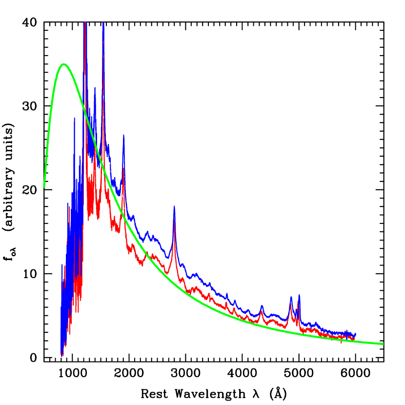
Figure 8: Bright SDSS QSO spectral composite [blue], faint SDSS QSO spectral composite [red], and the continuum of a standard disk (up to a normalizing constant) corresponding to a characteristic temperature of $T^{*}=92,700\,{\rm K}$ [green] (see Figure 7). Although the standard disk model determines an excellent fit to the composite residual (Table 1, Figure 7); when the fit is applied to the composite continuum (rather than to the residual), the disk continuum tends to underestimate the observed continuum around $\sim 3000\hbox{\rm\AA}$ (corresponding to the “small blue bump”), and to overestimate at shorter wavelengths.

In Figure 8 we show the bright SDSS QSO spectral composite and the faint SDSS QSO spectral composite (Wilhite et al., 2005), superimposed with the continuum of a standard disk (up to a normalizing constant) corresponding to a characteristic temperature of $T^{*}=92,700\,{\rm K}$. When the accretion disk fit is applied to the composite continuum (rather than to the residual), while roughly reproducing the overall UV/optical continuum, it does not present such an excellent agreement with observations as it does with the composite residual (Figure 7). Within the context of the models that are applied here, this is due to the contribution of non-variable sources that do not originate directly from the accretion disk. For example, the disk model continuum tends to underestimate the observed emission around $\sim 3000\hbox{\rm\AA}$, corresponding to the “small blue bump” emission, which is probably composed mainly of Balmer continuum emission and Fe line complexes.

5 Summary and Conclusions

Under the assumption that the UV/optical variability in QSOs is due to a change of mass accretion rate in a standard disk, we have analyzed a composite QSO residual spectrum constructed from hundreds of objects observed by the SDSS. An advantage of using difference spectra is the ability to remove non-variable components from the analysis. We have shown that our analysis technique can recover disk parameters in simulated data. The model is relatively simple — the shape of the difference spectrum depends only on the disk characteristic temperature $T^{*}$.

Our main conclusion is that on average (i.e., through the SDSS composite), in the wavelength range 1300-6000Å, residual QSO spectra can be quantitatively accounted for by a standard thermal disk that has varied from one steady state to another steady state by changing its mass accretion rate.

In turn, this suggests that most of the UV/optical variability may be due to processes involving the disk, and that a significant fraction of the UV/optical spectrum may come directly from the disk as has been suggested by many different authors.

We are currently studying individual QSO spectra taken from the SDSS. If the analysis shows consistency with individual objects, as it has done here for composite spectra, then we may have a method to probe the inner disk region by analyzing the difference between variable EUV and the standard disk model predictions. Also, if this method can be used with higher order terms, then there is a possibility of separating and determining black hole mass $M_{bh}$ and disk mass accretion rate $\dot{M}_{accr}$, for direct comparison with other methods of measuring these parameters.

Table 1: Accretion Disk Fits to the Composite Residual Spectrum

$\lambda$ (Å)	Excluded Lines	$\bar{T}^{*}$ (K)	2 $\sigma_{\bar{T}^{*}}$ (K)	$\chi^{2}/n$
800 - 6000	$\cdots$	80,100	400	4.892
912 - 6000	$\cdots$	82,400	400	4.695
1300 - 6000	$\cdots$	95,500	700	3.345
1300 - 1500,	C IV 1549Å	$\cdots$	$\cdots$	$\cdots$
1600 - 6000	$\cdots$	91,500	700	3.111
1300 - 1500,	C IV 1549Å	$\cdots$	$\cdots$	$\cdots$
1600 - 2750,	Mg II 2798Å	$\cdots$	$\cdots$	$\cdots$
2850 - 6000	$\cdots$	91,700	700	3.155
1300 - 1500,	C IV 1549Å	$\cdots$	$\cdots$	$\cdots$
1600 - 2750,	Mg II 2798Å	$\cdots$	$\cdots$	$\cdots$
2850 - 4810,	H$\beta$ 4861Å	$\cdots$	$\cdots$	$\cdots$
4910 - 6000	$\cdots$	92,700	700	2.965
1300 - 1500,	C IV 1549Å	$\cdots$	$\cdots$	$\cdots$
1600 - 2750,	Mg II 2798Å	$\cdots$	$\cdots$	$\cdots$
2850 - 4810,	H$\beta$ 4861Å	$\cdots$	$\cdots$	$\cdots$
4910 - 5825,	He I 5875Å	$\cdots$	$\cdots$	$\cdots$
5925 - 6000	$\cdots$	92,700	700	2.993

Figure 3: $\bar{T}^{*}$ estimated through the method discussed in §3.2 for “simulated” data between rest frame wavelengths of 1300Å and 6000Å, that is, for simulated data representing the exact residual flux from the standard disk model (§2). The exact value of $\bar{T}^{*}$ is $70,000\,{\rm K}$, and a measurement error of 5% on the simulated density flux measurements of the bright and faint phase is assumed. For the above parameters, accurate values for $\bar{T}^{*}$ are obtained for variations in temperature of up to $\Delta T\approx 15,000\,{\rm K}$. That is, the method estimates accurate values for $\bar{T}^{*}$ (for the parameters used here) for changes in mass accretion rate $\dot{M}_{accr}$ of up to approximately a factor of two [see eq. (26)]. The reason that the characteristic temperature $\bar{T}^{*}$ becomes overestimated for larger variations in temperature $\Delta T^{*}$, is that the third and higher order terms of equation (36) are no longer negligible.

Figure 4: Standard deviation $\sigma_{\bar{T}^{*}}$ on the estimated value of $\bar{T}^{*}$ obtained through the method discussed in §3.2 for “simulated” data as described in and for the same physical parameters of Figure 3. The exact value of $\bar{T}^{*}$ is $70,000\,{\rm K}$. For the above physical parameters, the standard deviation $\sigma_{\bar{T}^{*}}$ is less than $15,000\,{\rm K}$ for values of $\Delta T^{*}$ greater than $\approx 250\,{\rm K}$. The reason that $\sigma_{\bar{T}^{*}}$ becomes significantly large (i.e., comparable to the value of $\bar{T}^{*}$) at very low temperature variations $\Delta T^{*}$, is that errors on the flux measurements of the bright and faint phases become larger than the residual flux.

Figure 5: Rest frame time lag histogram of the SDSS QSO object sample used in the contruction of the composite residual spectrum. The median rest frame time lag is 124.5 days, and the full sample ranges from 17.5 to 270.4 days.

.

References

- Abazajian et al. (2005) Abazajian, K., et al. 2005, AJ, 129, 1755
- Bardeen, Press, & Teukolsky (1972) Bardeen, J. M., Press, W. H., & Teukolsky, S. A. 1972, ApJ, 178, 347
- Blanton et al. (2003) Blanton, M. R., Lin, H., Lupton, R. H., Maley, F. M., Young, N., Zehavi, I., & Loveday, J. 2003, AJ, 125, 2276
- Camenzind & Courvoisier (1984) Camenzind, M., Courvoisier, T. J.-L. 1984, A&A, 140, 341
- Colemann & Shields (1993) Colemann, H. H., & Shields, G. A. 1993, Rev. Mexicana Astron. Astrofis., 27, 95
- Cutri et al. (1985) Cutri, R. M., Wiśniewski, W. Z., Rieke, G. H., & Lebofsky, M. J. 1985, ApJ, 296, 423
- Czerny & Elvis (1987) Czerny, B., & Elvis, M. 1987, ApJ, 321, 305
- Czerny et al. (2003) Czerny, B., Nikolajuk M., Różańska, A., Dumont, A.-M., Loska, Z., & Życki, P. T. 2003, A&A, 412, 317
- Dörrer et al. (1996) Dörrer, T., Riffert, H., Staubert, R., & Ruder, H. 1996, A&A, 311, 69.
- Edelson, Krolik, & Pike (1990) Edelson, R. A., Krolik, J. H., & Pike, G. F. 1990, ApJ, 359, 86
- Elvis et al. (1986) Elvis, M., Green, R. F., Bechtold, J., Schmidt, M., Neugebauer, G., Soifer, B. T., & Mathews, K. 1986, ApJ, 310, 291
- Elvis et al. (1994) Elvis, M., Wilkes, B. J., McDowell, J. C., Green, R. F., Bechtold, J., Willner, S. P., Oey, M. S., Polomski, E., & Cutri, R. 1994, ApJS, 95, 1
- Fiore et al. (1995) Fiore, F., Elvis, M., Siemiginowska, A., Wilkes, B. J., McDowell, J. C., & Mathur, S. 1995, ApJ, 449, 74
- Frank, King & Raine (1992) Frank, J., King, A., & Raine, D. 1992, Accretion Power in Astrophysics (Cambridge University Press)
- Fukugita et al. (1996) Fukugita, M., Ichikawa, T., Gunn, J. E., Doi, M., Shimasaku, K., and Schneider, D. P. 1996, AJ, 111, 1748
- Gu et al. (2001) Gu, M., Cao, X., Jiang, D. R., Xu, Y. 2001, MNRAS, 321, 369
- Gunn et al. (1998) Gunn, J. E. et al. 1998, AJ, 116, 3040
- Hogg et al. (2001) Hogg, D. W., Finkbeiner, D. P., Schlegel, D. J., & Gunn, J. E. 2001, AJ, 122, 2129
- Hubeny et al. (2000) Hubeny, I., Agol, E., Blaes, O., & Krolik, J. H. 2000, ApJ, 533, 710
- Hubeny et al. (2001) Hubeny, I., Blaes, O., Krolik, J. H., & Agol, E. 2001, ApJ, 559, 680
- Ivezic et al. (2004) Ivezic, Z., et al. 2004, AN, 325, 583
- Kinney et al. (1991) Kinney, A. L., Bohlin, R. C., Blades, J. C., & York, D. G. 1991, ApJS, 75, 645
- Krolik et al. (1991) Krolik, J. H., Horne, K., Kallman, T. R., Malkan, M. A., & Edelson, R. A. 1991, ApJ, 371, 541
- Krolik (1999) Krolik, J. H. 1999, Active Galactic Nuclei: From the Central Black Hole to the Galactic Environment (Princeton University Press)
- Laor & Netzer (1989) Laor, A., & Netzer, H. 1989, MNRAS, 238, 897
- Laor (1990) Laor, A. 1990, MNRAS, 246, 369
- Lin & Papaloizou (1996) Lin, D. N. C., & Papaloizou, J. C. B. 1996, ARA&A, 34, 703
- Malkan & Sargent (1982) Malkan, M., & Sargent, W. 1982, ApJ, 254, 22
- Malkan (1983) Malkan, M. A. 1983, ApJ, 268, 582
- Mirabel & Rodríguez (1999) Mirabel, I. F., & Rodríguez, L. F. 1999, ARA&A, 37, 409
- Natali et al. (1998) Natali, F., Giallongo, E., Cristiani, S., & La Franca, F. 1998, AJ, 115, 397
- Novikov & Thorne (1973) Novikov, I. D., & Thorne, K. S. 1973, in Black Holes, eds. C. De Witt and B. De Witt (New York: Gordon and Breach)
- Page & Thorne (1974) Page, D. N., & Thorne, K. S. 1974, ApJ, 191, 499
- Paltani & Courvoisier (1994) Paltani, S., & Courvoisier, T. J.-L. 1994, A&A, 291, 74
- Pier et al. (2003) Pier, J. R., Munn, J. A., Hindsley, R. B., Hennessy, G. S., Kent, S. M., Lupton, R. H., & Ivezic, Z. 2003, AJ, 125, 1559
- Pringle (1981) Pringle, J. E. 1981, ARA&A, 19, 137
- Richards et al. (2002) Richards, G. T. et al. 2002, AJ, 123, 2945
- Ross, Fabian, & Mineshige (1992) Ross, R. R., Fabian, A. C., & Mineshige, S. 1992, MNRAS, 258, 189
- Sanders et al. (1989) Sanders, D. B., Phinney, E. S., Neugebauer, G., Soifer, B. T., & Mathews, K. 1989, ApJ, 347, 29
- Shakura & Sunyaev (1973) Shakura, N. I., & Sunyaev, R. A. 1973, A&A, 24, 337
- Shalyapin et al. (2002) Shalyapin, V. N., Goicoechea, L. J., Alcalde, D., Mediavilla, E., Muñoz, J. A., & Gil-Merino, R. 2002, ApJ, 579, 127
- Schneider et al. (2003) Schneider, D. P. et al. 2003, AJ, 126, 2579
- Shields (1978) Shields, G. A. 1978, Nature, 272, 706
- Shields & Colemann (1994) Shields, G. A., Colemann, H. H. 1994, in NATO Advanced Research Workshop on Theory of Accretion Disks - 2 ed. W. Duschl et al. (Dordrecht: Kluwer), 223
- Sirola et al. (1998) Sirola, C. J., Turnshek, D. A., Weymann, R. J., Monier, E. M., Morris, S. L., Roth, M. R., Krzeminski, W., Kunkei, W. E., Duhalde, O., & Sheaffer, S. 1998, ApJ, 495, 659
- Smith et al. (2002) Smith, J. A. et al. 2002, AJ, 123, 2121
- Störzer, Hauschildt, & Allard (1994) Störzer, H., Hauschildt, P. H., & Allard, F. 1994, ApJ, 437, L91
- Stoughton et al. (2002) Stoughton, C. et al. 2002, AJ, 123, 485
- Sun & Malkan (1989) Sun, W.-H., & Malkan, M. A. 1989, ApJ, 346, 68
- Ulrich, Maraschi, & Urry (1997) Ulrich, M.-H., Maraschi, L., & Urry, C. M. 1997, ARA&A, 35, 445
- Vanden Berk et al. (2004) Vanden Berk, D. E., Wilhite, B. C., Kron, R. G., Anderson, S. F., Brunner, R. J., Hall, P. B., Ivezić Z̆., Richards, G. T., Schneider, D. P., York, D. G., Brinkman, J. V., Lamb, D. Q., Nichol, R. C., & Schlegel, D. J. 2004, ApJ, 601, 692
- Wandel & Petrosian (1988) Wandel, A., & Petrosian, V. 1988, ApJ, 329, L11
- Webb & Malkan (2000) Webb, W., & Malkan, M. 2000, ApJ, 540, 652
- Wilhite et al. (2005) Wilhite, B. C., Vanden Berk, D. E., Kron, R. G., & Pereyra, N. A. 2005, ApJ, submitted
- York et al. (2000) York, D. G. et al. 2000, AJ, 120, 1579