Broad-band colors and overall photometric properties of template galaxy models from stellar population synthesis

Abstract

We present here a new set of evolutionary population synthesis models for template galaxies along the Hubble morphological sequence. The models, that account for the individual evolution of the bulge, disk, and halo components, provide basic morphological features, along with bolometric luminosity and color evolution (including Johnson/Cousins, Gunn $g,r,i$, and Washington $C,M,T_{1},T_{2}$ photometric systems) between 1 and 15 Gyr. Luminosity contribution from residual gas is also evaluated, both in terms of nebular continuum and Balmer-line enhancement.

Our theoretical framework relies on the observed colors of present-day galaxies, coupled with a minimal set of physical assumptions related to SSP evolution theory, to constrain the overall distinctive properties of galaxies at earlier epochs. A comparison with more elaborated photometric models, and with empirical sets of reference SED for early- and late-type galaxies is accomplished, in order to test output reliability and investigate internal uncertainty of the models.

The match with observed colors of present-day galaxies tightly constrain the stellar birthrate, $b$, that smoothly increases from E to Im types. The comparison with observed SN rate in low-redshift galaxies shows, as well, a pretty good agreement, and allows us to tune up the inferred star formation activity and the SN and Hypernova rates along the different galaxy morphological types. Among others, these results could find useful application also to cosmological studies, given for instance the claimed relationship between Hypernova events and Gamma-ray bursts.

One outstanding feature of model back-in-time evolution is the prevailing luminosity contribution of the bulge at early epochs. As a consequence, the current morphological look of galaxies might drastically change when moving to larger distances, and we discuss here how sensibly this bias could affect the observation (and the interpretation) of high-redshift surveys.

In addition to broad-band colors, the modeling of Balmer line emission in disk-dominated systems shows that striking emission lines, like $H\alpha$, can very effectively track stellar birthrate in a galaxy. For these features to be useful age tracers as well, however, one should first assess the real change of $b$ vs. time on the basis of supplementary (and physically independent) arguments.

1 Introduction

Since its early applications to extragalactic studies (Spinrad & Taylor, 1971; Tinsley & Gunn, 1978), stellar population synthesis has been the natural tool to probe galaxy evolution. The works of Searle et al. (1973) and Larson (1975) provided, in this sense, a first important reference for a unitary assessment of spectrophotometric properties of early- and late-type systems in the nearby Universe, while the contribution of Bruzual & Kron (1980), Lilly & Longair (1984), Yoshii & Takahara (1988), among others, represent a pionering attempt to extend the synthesis approach also to unresolved galaxies at cosmological distances.

In this framework, color distribution along the Hubble sequence has readily been recognized as the most direct tracer for galaxy diagnostics; a tight relationship exists in fact between integrated colors and morphological type, through the relative contribution of bulge and disk stellar populations (Köppen & Arimoto, 1990; Arimoto & Jablonka, 1991). Ongoing star formation, in particular, is a key mechanism to modulate galaxy colors, especially at short wavelength (Larson & Tinsley, 1978; Kennicutt, 1998), while visual and infrared luminosity are better sensitive to the global star formation history (Quirk & Tinsley, 1973; Sandage, 1986; Gavazzi & Scodeggio, 1996). External environment conditions could also play a role, as well as possible interactions of galaxies with embedding giant haloes, like in some CDM schemes (Firmani & Tutukov, 1992, 1994; Pardi & Ferrini, 1994).

In this work I want to try a simple heuristic approach to galaxy photometric evolution relying on a new family of theoretical template models to account for the whole Hubble morphological sequence. Galaxy evolution is tracked here in terms of the individual history of the composing sub-systems, including the bulge, disk and halo; the present discussion completes the analysis already undertaken in an accompanying paper (Buzzoni, 2002, hereafter Paper I), and relies on the evolutionary population synthesis code developed previously (Buzzoni, 1989, 1995, hereafter B89 and B95, respectively).

A main concern of this work is to provide the user with a quick reference tool to derive broad-band colors and main morphological parameters of galaxies allover their “late” evolutionary stages (i.e. for $t\ga 1$ Gyr). This should be the case for most of $z\la 3$ systems, for which the formation event is mostly over and the morphological design already in place.

Within minor refinements, the present set of models has already been successfully used by Massarotti et al. (2001) in their photometric study of the Hubble Deep Field galaxies; a further application of these templates is also due to Buzzoni et al. (2005), to assess the evolutionary properties of the planetary nebula population in bright galaxies and the intracluster medium. Compared to other more “physical” (and entangled) approaches, I believe that a major advantage of this simplified treatment is to allow the user maintaining a better control of the theoretical output, and get a direct feeling of the changes in model properties as far as one or more of the leading assumptions are modified.

Models will especially deal with the stellar component, which is obviously the prevailing contributor to galaxy luminosity. Residual gas acts more selectively on the integrated spectral energy distribution (SED) by enhancing monochromatic emission, like for the Balmer lines. As far as galaxy broad-band colors are concerned, in the present age range, its influence is negligible and can be treated apart in our discussion. Internal dust could play, on the contrary, a more important role, especially at short wavelength ($\lambda\la 3000$ Å). Its impact for high-redshift observations has been discussed in some detail in Paper I.

In this paper we will first analyze, in Sec. 2, the basic components of the synthesis model, taking the Milky Way as a main reference to tune up some relevant physical parameters for spiral galaxies. A set of color fitting functions is also given in this section, in order to provide the basic analytical tool to compute galaxy luminosity for different star formation histories.

Model setup is considered in Sec. 3, especially dealing with the disk physical properties; metallicity and stellar birthrate will be constrained by comparing with observations and other theoretical studies. In Sec. 4 we will assemble our template models, providing colors and other distinctive features for each galaxy morphological type along the Hubble sequence, from E to Im. A general sketch of back-in-time evolution is outlined in this section, focussing on a few relevant aspects that deal with the interpretation of high-redshift data. Section 5 discusses the contribution of the residual gas; we will evaluate here the nebular luminosity and derive Balmer emission-line evolution. The main issues of our analysis are finally summarized in Sec. 6.

2 Operational tools

Our models consist of three main building blocks: we will consider a central bulge, a disk, and an external halo. It is useful to track evolution of each block individually, in terms of composing simple stellar populations (SSPs), taking advantage of the powerful theoretical formalization by Tinsley (1980) and Renzini & Buzzoni (1986).

If SSP evolution is known and a star formation rate (SFR) can be assumed vs. time, the general relation for integrated luminosity of a stellar system is

$$L_{\rm gal}(t)=\int_{0}^{t}L_{\rm SSP}(\tau)\ SFR(t-\tau)\ d\tau.$$ (1)

Operationally, the integral in eq. (1) is computed by discrete time steps, $\Delta\tau$, taking the lifetime of the most massive stars in the initial mass function (IMF), $t_{\rm min}$, as a reference, so that $\Delta\tau=t_{\rm min}$.

In a closed-box evolution, galaxy SFR is expected to be a decreasing function of time (e.g. Tinsley, 1980; Arimoto & Yoshii, 1986); on the other hand, if fresh gas is supplied from the external environment, then an opposite trend might even be envisaged. One straighforward way to account for this wide range of evolutionary paths is to assume a power law such as SFR $=K\ t^{-\eta}$, with $\eta<1$.

As we pointed out in Paper I, an interesting feature of this simple parameterization is that stellar birthrate,

$$b={{{\rm SFR}(t)}\over{\langle{\rm SFR}\rangle}}=(1-\eta),$$ (2)

is a time-independent function of SFR and becomes therefore an intrinsic distinctive parameter of the galaxy model.

2.1 SSP evolution

In order to properly apply eq. (1) to the different evolutionary cases, we need first to secure its basic “ingredient” by modeling SSP luminosity evolution. The original set of B89 and B95 population synthesis models, and its following upgrade and extension as in Paper I, especially dealt with evolution of low- and intermediate-mass stars, with $M\la 2~{}M_{\odot}$ and main sequence (MS) lifetime typically greater than 1 Gyr. As a striking feature in this mass range, red giant branch sets on in stars with a degenerate Helium core, tipping at high luminosity ($\log L/L_{\odot}\sim 3.3$) with the so-called Helium-flash event Sweigart & Gross (1978).

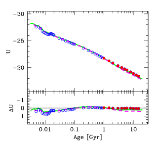
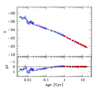
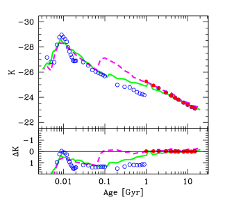
Figure 1: Upper plots of each panel: luminosity evolution of present SSP models (solid dots), for solar metallicity and Salpeter IMF, is compared with other theoretical outputs according to Leitherer et al. (1999, open dots), Bressan et al. (1994, dashed line), and Bruzual & Charlot (2003, solid line). Total mass is scaled to $M_{\rm SSP}=10^{11}~{}M_{\odot}$ throughout, with stars in the range between 0.1–120 $M_{\odot}$. The Leitherer et al. (1999) model has been slightly increased in luminosity (by about 0.06 mag in bolometric, at 1 Gyr) to account for the missing luminosity contribution from low-MS stars ($M_{*}\leq 1.0~{}M_{\odot}$).
Lower plots of each panel: model residuals with respect to the fitting functions of Table 1. See text for discussion.

For younger ages (i.e. $t\la 1$ Gyr), evolution is less univocally constrained, as convection and mass loss via stellar winds (both depending on metallicity) sensibly modulate the evolutionary path of high-mass stars across the H-R diagram on timescales as short as $\sim 10^{6}$ yr (de Loore, 1988; Maeder & Conti, 1994). Such a quicker Post-MS evolution could also lead to a biased sampling of stars in the different phases, even at galaxian mass-scale, inducing intrinsic uncertainties in the SSP spectrophotometric properties independently of the input physics details (see Cerviño et al., 2002 and Cerviño & Valls-Gabaud, 2003, for a brilliant assessment of this problem).

A combined comparison of different SSP models, over the full range of stellar masses, is displayed in Fig. 1, where we matched our SSP model sequence for solar metallicity and Salpeter (1955) IMF with the corresponding theoretical output from Leitherer et al. (1999), Bressan et al. (1994) and Bruzual & Charlot (2003, their “Padova 1994” isochrone setup). Luminosity in the Johnson $U$, $V$, $K$ bands, and in bolometric as well, is explored in the four panels of the figure, referring to evolution of a $10^{11}~{}M_{\odot}$ SSP, with stars in the range $0.1\leq M_{*}/M_{\odot}\leq 120$. To consistently compare with the other outputs, the Leitherer et al. models have been slightly increased in luminosity (by some $\Delta{\rm mag}=-0.06$ in bolometric at 1 Gyr) to account for the missing low-MS ($M_{*}<1~{}M_{\odot}$) contribution, according to the B89 estimates.

Figure 1 shows a remarkable agreement between the four theoretical codes; in particular, ultraviolet and bolometric evolution is fairly well tracked over nearly four orders of magnitude of SSP age. The lack of AGB evolution in the Leitherer et al. (1999) code is, however, especially evident in the $K$ plot, where a glitch of about 1 mag appears at the match with our model sequence about $t\sim 1$ Gyr. To a lesser extent, also the $K$-band contribution of red giant stars seems to be partly undersized in the Bruzual & Charlot (2003) models between $10^{8}$ and $10^{9}$ yrs, probably be due to interpolation effects across stellar tracks in the relevant range of mass (i.e. $M_{*}=5\to 2~{}M_{\odot}$).

Table 1: SSP magnitude fitting functions^(a)

Band	$\lambda_{\it eff}$	$\log f_{o}^{(b)}$	mag = $(\alpha^{\prime}+\alpha^{\prime\prime}{\rm[Fe/H]})\log t_{9}+\beta{\rm[Fe/H]}+\gamma+\delta({\rm t}_{9},{\rm[Fe/H]})$					$\sigma$	System
	[Å]	[erg s-1 cm-2 Å-1]	$\alpha^{\prime}$	$\alpha^{\prime\prime}$	$\beta$	$\gamma$	$\delta({\rm t}_{9},{\rm[Fe/H]})$	[mag]
U	3650	–8.392	2.743	0.26	0.006	2.872	+0.09 10[Fe/H]	$\pm 0.026$	Johnson
C	3920	–8.275	2.560	0.16	–0.024	2.853	+0.09 10[Fe/H]	$\pm 0.022$	Washington
B	4420	–8.205	2.390	0.08	0.033	2.909		$\pm 0.020$	Johnson
M	5060	–8.351	2.232	0.08	–0.060	2.477		$\pm 0.020$	Washington
g	5170	–8.384	2.214	0.08	–0.069	2.401		$\pm 0.019$	Gunn
V	5500	–8.452	2.163	0.08	–0.094	2.246		$\pm 0.019$	Johnson
T1	6310	–8.632	2.072	0.08	–0.160	1.835		$\pm 0.019$	Washington
RC	6470	–8.670	2.048	0.08	–0.176	1.756		$\pm 0.019$	Cousins
r	6740	–8.527	2.037	0.08	–0.189	2.147		$\pm 0.019$	Gunn
R	7170	–8.790	2.006	0.08	–0.207	1.546		$\pm 0.019$	Johnson
IC	7880	–8.936	1.977	0.08	–0.275	1.226		$\pm 0.019$	Cousins
T2	7940	–8.938	1.972	0.08	–0.255	1.250		$\pm 0.019$	Washington
i	8070	–8.653	1.969	0.08	–0.259	1.981		$\pm 0.019$	Gunn
I	9460	–9.136	1.923	0.08	–0.327	0.944		$\pm 0.020$	Johnson
J	12500	–9.526	1.863	0.08	–0.444	0.333		$\pm 0.018$	Johnson
H	16500	–9.965	1.833	0.08	–0.551	–0.375		$\pm 0.016$	Johnson
K	22000	–10.302	1.813	0.08	–0.614	–0.561		$\pm 0.016$	Johnson
Bol			1.923		–0.324	1.623	$-0.1\,t_{9}^{-0.5}$	$\pm 0.014$

^(a) For a Salpeter IMF with stars in the mass range $0.1\leq M/M_{\odot}\leq 120$.

^(b) $\log f=-0.4\,{\rm mag}+\log f_{o}$. For the bolometric: $\log L/L_{\odot}=-0.4\,({\rm Bol}-4.72)$.

Definitely, SSP evolution appears to be best tracked by the isochrone-synthesis models of Bressan et al. (1994); like in our code, these models meet the prescriptions of the so-called “Fuel Consumption Theorem” (Renzini & Buzzoni, 1986), and self-consistently account for the AGB energetic budget down to the onset of the SN II events (about $t\simeq 10^{8}$ yr). In any case, as far as early SSP evolution is concerned, a combined analysis of Fig. 1 makes clear the intrinsic uncertainty of the synthesis output in this particular age range, mainly as a result of operational and physical differences in the treatment of Post-MS evolution (cf. Charlot et al., 1996, for further discussion on this subject).

2.2 SSP fitting functions

Model setup, like in case of composite stellar populations according to eq. (1), would be greatly eased if we could manage the problem semi-analytically, in terms of a suitable set of SSP magnitude fitting functions. An important advantage in this regard is that also intermediate cases for age and/or metallicity could readily be accounted for in our calculations.

For this task we therefore considered the B89 and B95 original dataset of SSP models (and its further extension, as in Paper I), with Salpeter IMF and red horizontal branch morphology (cf. B89 for details). In addition to the original Johnson photometry, we also included here the Cousins ($R_{C},I_{C}$), Gunn ($g,r,i$), and Washington ($C,M,T_{1},T_{2}$) band systems. The works of Bessell (1979), Thuan & Gunn (1976), Schneider et al. (1983), and Canterna (1976) have been referred to for the different system definition (see also Cellone & Forte, 1996, for an equivalent calibration of the Washington colors based on the B89 models). Our analysis will therefore span a wide wavelength range, from 3600 Å ($U$ band), to 2.2 $\mu m$ ($K$ band), sampling SSP luminosity at roughly $\Delta\lambda\sim 400$ Å steps in the spectral window between 3600–9000 Å.

For SSP magnitude evolution, a general fit was searched for in the form

$${\rm mag}=(\alpha^{\prime}+\alpha^{\prime\prime}\,{\rm[Fe/H]})\ \log t_{9}+\beta\ {\rm[Fe/H]}+\gamma+\delta({\rm t}_{9},{\rm[Fe/H]}),$$ (3)

where $t_{9}$ is SSP age, expressed in Gyr. The whole set of the fitting coefficients is summarized in Table 1 (columns 4 to 8); note that the $U$ magnitude scale in the table already accounts for the corrections devised in B95. Column 2 of the table reports the effective wavelength for each photometric passband, as directly computed from the adopted filter profile.

Mass scaling for the SSP fitting functions in Table 1 can be done by adding to all magnitudes an offset

$$\Delta{\rm mag}=-2.5\log M_{\rm tot}+2.5\log(M/L_{\rm V})_{15},$$ (4)

where both SSP total mass and the V-band mass-to-light ratio (estimated at $t=15$ Gyr) are in solar units. A quite accurate fit (within a $\pm 1.5$% relative scatter) for the latter quantity over the metallicity range of our models is:

$$\left({M\over{L_{\rm V}}}\right)_{15}=3.23\ ({\rm[Fe/H]}+1.5)^{2}+6.41.$$ (5)

Again, the fit holds for stars in the range 0.1–120 $M_{\odot}$ and a Salpeter IMF.

The whole set of fitting functions in Table 1 is optimized in the range [Fe/H] $=[-1.5,+0.5]$. For $t\geq 1$ Gyr, model grid is fitted with an internal accuracy better than $\pm 0.02$ mag, slightly worsening in the ultraviolet, as reported in column 9 of the table.

The residual trend of the Leitherer et al. (1999), Bressan et al. (1994) and Bruzual & Charlot (2003) SSP models with respect to our fitting functions is displayed in the lower plot of each panel of Fig. 1. Reference equations give a fully adequate description of SSP luminosity evolution well beyond the nominal age limits of our model grid, and span the whole range of AGB evolution, for $t\geq 10^{8}$ yr. At early epochs, of course, fit predictions partially miss the drop in the SSP integrated luminosity, when core-collapsed evolution of high-mass stars ends up as a SN burst thus replacing the standard AGB phase (we will return on this important feature in Sec. 4.1). As far as composite stellar populations are concerned, however, the induced uncertainty of fit extrapolation on the total luminosity of the system is much reduced since eq. (1) averages SSP contribution over time.

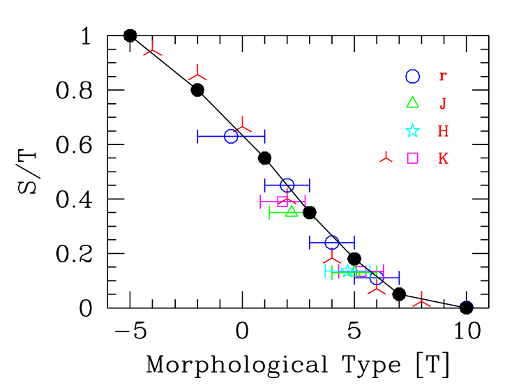
Figure 2: The adopted red/infrared calibration for the S/T morphological parameter, defined as $L_{\rm spheroid}/L_{\rm tot}$ ($\bullet$ markers), as derived from the data of Kent (1985; $\circ$ markers), de Jong (1996; reversed “Y” markers), Giovanardi & Hunt (1988; $\sq$, $\triangle$ and $\star$ markers for later-type spirals at $T\sim 5$), and Moriondo et al. (1998; $\triangle$ and $\sq$ markers for early-type spirals, about $T\sim 2$). Photometric bands of observations are labeled top right in the plot.

3 Model setup: the basic building blocks

To consistently assemble the three main building blocks of our synthesis models we mainly relied on the Kent (1985) galaxy decomposition profiles, that probe the spheroid (i.e. bulge+halo) vs. disk luminosity contribution at red wavelength (Gunn $r$ band). Kent’s results substantially match also the near-infrared observations (see Fig. 2), while $B$ luminosity profiles (Simien & de Vaucouleurs, 1986) tend in general to show a slightly enhanced disk component in later-type spirals, as a consequence of a bluer color with respect to the bulge.

For each Hubble type we eventually calibrated a morphological parameter defined as S/T $=L{\rm(spheroid)}/L{\rm(tot)}$. As the S/T calibration does not vary much at visual and infrared wavelength, we fixed the $I$ luminosity as a reference for model setup. This also fairly traces the bolometric partition (cf. the corresponding fitting coefficients of Table 1), especially for early-type spirals. According to the observations, the luminous mass of the disk remains roughly constant along the Sa–Im sequence, while bulge luminosity decreases towards later-type spirals (Simien & de Vaucouleurs, 1983; Gavazzi, 1993).

3.1 The spheroid sub-system

There is general consensus on the fact that both the halo and bulge sub-systems in the Galaxy basically fit with coeval SSPs older than $\sim 13$ Gyr (Gilmore et al., 1990; Renzini, 1993; Frogel, 1999; Feltzing & Gilmore, 2000). Observations of the central bulge of the Milky Way show that it mostly consists of metal-rich stars (Frogel, 1988, 1999) and this seems a quite common situation also for external galaxies (Jablonka et al., 1996; Goudfrooij et al., 1999; Davidge, 2001). The exact amount of bulge metallicity, however, has been subject to continual revision in the recent years, ranging from a marked metal overabundance (i.e. [Fe/H] $\sim+0.2$; Whitford & Rich, 1983; Rich, 1990; Geisler & Friel, 1992) to less prominent values, actually consistent with a standard or even slightly sub-solar metallicity (Tiede et al., 1995; Sadler et al., 1996; Zoccali et al., 2003; Origlia & Rich, 2005).

On the contrary, the halo mostly consists of metal-poor stars (Zinn, 1980; Sandage & Fouts, 1987), and its metallicity can be probed by means of the globular cluster environment. From the complete compilation of 149 Galactic globular clusters by Harris (1996), for instance, we derive a mean [Fe/H] $=-1.24\pm 0.56$, with clusters spanning a range $-2.3\la$ [Fe/H] $\la 0.0$. This figure is in line with the inferred metallicity distribution of globular cluster systems in external galaxies (Brodie & Huchra, 1991; Durrell et al., 1996; Perrett et al., 2002; Kissler-Patig et al., 2005).

According to the previous arguments, for the spheroid component in our models we will adopt two coeval SSPs with [Fe/H]$=+0.22$ and $-1.24$, for bulge and halo, respectively. Once accounting for metallicity, via eq. (5) and Table 1, the standard halo/bulge mass ratio for the Milky Way (e.g. Sandage, 1987; Dwek et al., 1995) translates into a relative bolometric luminosity

$$[L_{\rm halo}:L_{\rm bulge}]=[15\%:85\%].$$ (6)

This partition will be adopted throughout in our models and provides a nearly solar luminosity-weighted metallicity for the spheroid system as a whole.

3.2 The disk

To set the disk distinctive parameters we need to suitably constrain stellar birthrate $b$ (or, equivalently, the SFR power-law index, $\eta$), and mean stellar metallicity along the Hubble morphological sequence. This could be done relying on the observed colors of present-day galaxies. In our analysis we will assume a current age of 15 Gyr.

The most exhaustive collection of photometric data for local galaxies definitely remains the RC3 catalog (de Vaucouleurs et al., 1991). Based on the original database of over 2500 objects, Buta et al. (1994) carried out a systematic analysis of the optical color distribution. Another comprehensive compilation from the RC3-UGC catalogs (1537 galaxies in total) is that of Roberts & Haynes (1994). Both data samples have been extensively discussed in Paper I; their analysis shows that a 1-$\sigma$ color scatter of the order of $\pm 0.15$ mag can be devised both for the $B-V$ and $U-B$ distributions as a realistic estimate of the intrinsic spread within each $T$ morphology class (cf. also Fukugita et al., 1995, on this point). This value should probably be increased by a factor of two for the infrared colors.

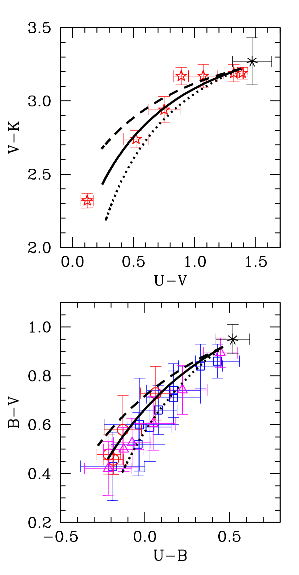
Figure 3: Two-color diagrams of galaxy distribution compared with 15 Gyr model sequences for different values of disk metallicity. Data are from Aaronson (1978, $\star$ markers), Pence (1976, $\circ$), Gavazzi et al. (1991, $\sq$), and Buta et al. (1994, $\triangle$). Mean colors for ellipticals (the $*$ marker in each panel) are from B95. In the models, a disk component is added as an increasing fraction of the total galaxy luminosity (in the sense of increasingly bluer colors). Long-dashed line is the theoretical locus for solar metallicity, while solid and dotted lines are for $[Fe/H]_{\rm disk}=-0.5$, and $-1.0$ dex, respectively.

3.2.1 Two-color diagrams and disk metallicity

A two-color diagram is especially suitable to constrain disk metallicity. Our experiments show in fact that any change in the stellar birthrate will shift the integrated colors along the same mean locus, for a fixed value of [Fe/H]. In Fig. 3, a set of disk model sequences with varying metallicity is compared with the $U,B,V,K$ photometry from the works of Pence (1976), Aaronson (1978), Gavazzi et al. (1991), and Buta et al. (1994). We only included those data samples with complete multicolor photometry avoiding to combine colors from different sources in the literature. The theoretical loci in the figure have been computed by adding to the same spheroid component an increasing fraction of disk luminosity, according to eq. (1) and assuming a SFR with $\eta=-0.8$. Three values for metallicity have been considered, namely [Fe/H] $=0.0,-0.5$, and –1.0 dex.

Both the $(U-V)$ vs. $(V-K)$ and $(U-B)$ vs. $(B-V)$ plots clearly point to a mean sub-solar metal content for the disk stellar component. This is especially constrained by late-type galaxies, where disk dominates total luminosity. We could tentatively adopt [Fe/H]${}_{\rm disk}=-0.5$ dex as a luminosity-weighted representative value for our models. As pointed out in Paper I, this value roughly agrees with the Milky Way stellar population in the solar neighborhood (Edvardsson et al., 1993), and is in line with the Arimoto & Jablonka (1991) theoretical estimates, suggesting a mean luminosity-weighted [Fe/H]${}_{\rm disk}\sim-0.3$ dex for their disk-dominated galaxy models. The intrinsic spread of the observations in Fig. 3, compared with the full range of the [Fe/H] loci, indicates however that metal abundance is not a leading parameter to modulate disk colors, and even a $\pm 0.3$ dex change in our assumptions would not seriously affect model predictions.

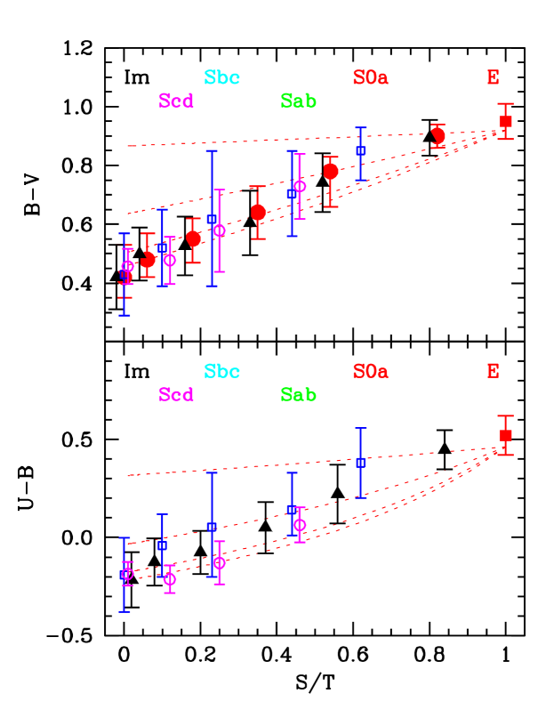
Figure 4: Galaxy color distribution vs. bolometric morphological parameter S/T $=L_{\rm spheroid}/L_{\rm tot}$ compared with 15 Gyr model sequences with fixed SFR power-law index. Data are from Pence (1976, $\circ$ markers), Gavazzi et al. (1991, $\sq$), Roberts & Haynes (1994, $\bullet$), and Buta et al. (1994, $\blacktriangle$). Mean colors for ellipticals ($\blacksquare$) are from B95. Dotted lines display the expected locus for models with three different values of the SFR index, namely $\eta=-0.8,0$, and +0.8 plus the SSP case, in the sense of increasingly redder colors. A trend is evident in the observations with a higher stellar birthrate for later-type systems.

3.2.2 Color distribution and disk SFR

Color distribution along with the S/T morphological parameter is a useful tool to constrain the disk SFR. This plot is in fact better sensitive to the relative amount of young vs. old stars in the galaxy stellar population, and gives an implicit measure of the disk birthrate, $b$. Our results are summarized in Fig. 4, comparing with the available $UBV$ photometry.

Four model sequences are displayed in each panel according to three different values of the SFR power-law index, namely $\eta=0.8,0.0,-0.8$ (i.e. $b=0.2,1,1.8$) plus the case of a plain SSP evolution. We adopted [Fe/H]${}_{\rm disk}=-0.5$ dex throughout in our calculations. Both the $B-V$ and $U-B$ plots indicate, in average, a higher stellar birthrate for later-type systems (Kennicutt et al., 1994). Our adopted calibration for $b$ vs. morphological type is shown in Fig. 8 of Paper I.

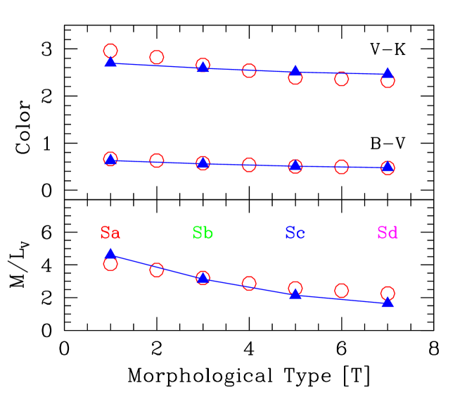
Figure 5: A comparison of our disk model output ($\blacktriangle$ markers) vs. the Arimoto & Jablonka (1991) original results ($\circ$ markers). The $V$-band M/L ratio (in solar units) refers to the stellar mass alone (i.e. the total mass converted to stars at the age of 15 Gyr); it has been normalized consistently, to account for the slightly different IMF mass range and slope (see text for discussion).

Table 2: Input distinctive parameters for 15 Gyr models

Hubble Type	$b^{(a)}$	$\eta$	S/T(b)	[Fe/H]
				[halo : disk : bulge]
E	0.0	SSP	1.00	–1.24           +0.22
S0	0.0	SSP	0.80	–1.24  –0.50  +0.22
Sa	0.2	$0.8$	0.55	–1.24  –0.50  +0.22
Sb	0.5	$0.5$	0.35	–1.24  –0.50  +0.22
Sc	0.9	$0.1$	0.18	–1.24  –0.50  +0.22
Sd	1.3	$-0.3$	0.05	–1.24  –0.50  +0.22
Im	1.8	$-0.8$	0.00	–0.50

^(a)Disk stellar birthrate
^(b)$S/T=L{\rm(spheroid)}/L{\rm(tot)}$ at red/infrared wavelength.

It is useful to compare our final results with the models of Arimoto & Jablonka (1991), which addressed disk chemio-photometric evolution in deeper detail. A slightly different IMF boundaries were adopted by Arimoto & Jablonka (1991) (i.e. a power-law index $s=2.45$ instead of our standard Salpeter value, $s=2.35$, and a stellar mass range $M_{*}=[0.05,\ 60]~{}M_{\odot}$ vs. our value of $M_{*}=[0.1,\ 120]~{}M_{\odot}$), so that we had to rescale their original values to consistently compare with our M/L ratio. Figure 5 shows a remarkable agreement with our results, along the whole late-type galaxy sequence, both in terms of integrated colors and stellar M/L ratio. To account for the missing luminosity of 60-120 $M_{\odot}$ stars in the Arimoto & Jablonka (1991) receipt, however, one should further decrease the inferred M/L ratio for their models in Fig. 5, especially for Sc-Sd systems.

4 Model output

The distinctive parameters eventually adopted for our galaxy templates, according to the previous discussion, have been collected in Table 2. A synoptic summary of the main output properties for 15 and 1 Gyr models is reported in Table 3. Compared with Paper I models, notice that we slightly revised here the bolometric luminosity scale as a consequence of a refined fitting function in Table 1. We therefore predict here a lower bolometric M/L ratio (because of a higher $L_{\rm bol}$ value), compared to Table 3 of Paper I. Apart from this difference, the change has no effect on the rest of the model properties as bolometric luminosity is a derived quantity for our calculations; full consistency is therefore preserved with the Paper I framework.

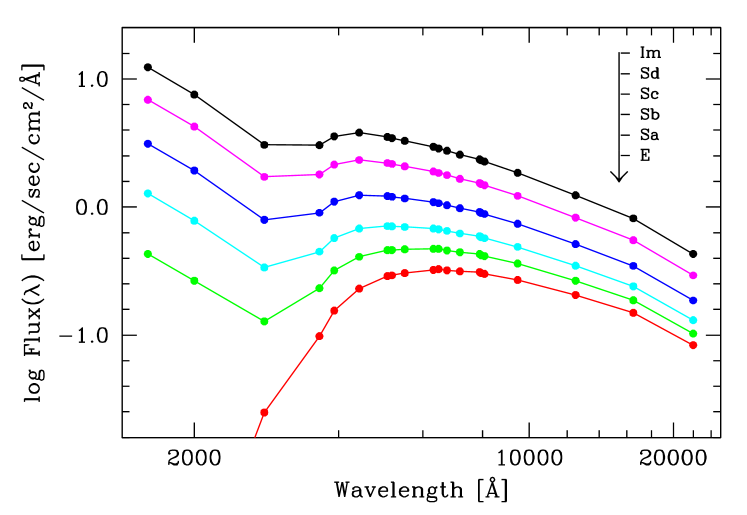
Figure 6: Theoretical SED for 15 Gyr template models of $M_{gal}=10^{11}~{}M_{\odot}$ along the Hubble sequence. Multicolor magnitudes have been converted to monocromatic flux density according to the photometric zero points of Table 1. The ultraviolet flux estimates at 1600, 2000, and 2800 Å are from Paper I.

Template galaxy models are described in full detail in the series of Table 6 to 12 of Appendix A, assuming a total mass $M_{\rm gal}=10^{11}$ M_⊙ for the system at 15 Gyr. In addition to the standard colors in the Johnson, Gunn and Washington photometric systems, also “composite” colors like $(g-V)$ and $(M-V)$ are reported in the tables in order to allow an easier transformation of photometry among the different systems. It could also be useful to recall, in this regard, that a straightforward transformation of the Johnson/Cousins magnitudes to the Sloan SDSS $(u^{\prime},g^{\prime},r^{\prime},i^{\prime},z^{\prime})$ photometric system can be obtained relying on the equations set of Fukugita et al. (1996, their eq. 23). A plot of the synthetic SED for 15 Gyr galaxies is displayed in Fig. 6 in a $\log$-$\log$ plot. Luminosity at different wavelength is obtained by converting theoretical magnitudes to absolute apparent flux, according to the photometric zero points of Table 1 (column 3). In the figure, ultraviolet magnitudes at 1600, 2000 and 2800 Å are from Paper I.

Table 3: Output summary for template galaxy models at 1 and 15 Gyr

	$\mid$  1 Gyr  $\mid$				$\mid$  15 Gyr  $\mid$
Hubble	S/T(a)	L/L${}_{\rm tot}^{(b)}$	M/M${}_{\rm tot}^{(c)}$	M/L(d)	S/T	L/Ltot	M/Mtot	M/L
Type		[halo : disk : bulge]	[halo : disk : bulge]			[halo : disk : bulge]	[halo : disk : bulge]
E	1.00	0.15  0.00  0.85	0.09  0.00  0.91	0.74	1.00	0.15  0.00  0.85	0.09  0.00  0.91	6.41
S0	0.81	0.12  0.19  0.69	0.08  0.16  0.76	0.71	0.81	0.12  0.19  0.69	0.08  0.16  0.76	6.14
Sa	0.66	0.10  0.34  0.56	0.08  0.17  0.75	0.59	0.52	0.08  0.48  0.44	0.07  0.26  0.67	4.48
Sb	0.62	0.09  0.38  0.53	0.07  0.13  0.80	0.53	0.30	0.04  0.70  0.26	0.05  0.37  0.58	3.06
Sc	0.65	0.10  0.35  0.55	0.08  0.08  0.84	0.53	0.14	0.02  0.86  0.12	0.04  0.51  0.45	1.86
Sd	0.56	0.08  0.44  0.48	0.08  0.09  0.83	0.47	0.04	0.01  0.96  0.03	0.02  0.77  0.21	1.05
Im	0.00	0.00  1.00  0.00	0.00  1.00  0.00	0.07	0.00	0.00  1.00  0.00	0.00  1.00  0.00	0.66
	[Fe/H]${}_{\rm tot}^{(e)}$	Disk colors	Integrated colors		[Fe/H]tot	Disk colors	Integrated colors
		(U–V) (B–V) (V–K)	(U–V) (B–V) (V–K)			(U–V) (B–V) (V–K)	(U–V) (B–V) (V–K)
E	$+0.00$		0.74   0.66   2.82		$+0.00$		1.38   0.92   3.22
S0	$-0.09$	0.60   0.60   2.55	0.71   0.64   2.77		$-0.09$	1.18   0.87   2.96	1.33   0.91   3.17
Sa	$-0.17$	0.20   0.43   2.34	0.53   0.58   2.68		$-0.24$	0.60   0.63   2.70	0.91   0.76   2.98
Sb	$-0.19$	0.10   0.38   2.27	0.47   0.55   2.66		$-0.34$	0.44   0.56   2.59	0.63   0.65   2.81
Sc	$-0.18$	0.01   0.34   2.20	0.45   0.55   2.66		$-0.43$	0.34   0.51   2.51	0.43   0.56   2.63
Sd	$-0.21$	–0.04   0.32   2.16	0.36   0.51   2.60		$-0.49$	0.28   0.48   2.46	0.31   0.49   2.50
Im	$-0.50$	–0.07   0.30   2.13	–0.07   0.30   2.13		$-0.50$	0.24   0.46   2.42	0.24   0.46   2.42

^(a)Bulge+ halo luminosity fraction in bolometric

^(b)Luminosity partition in bolometric

^(c)Mass partition of the stellar component

^(d)Stellar mass-to-light ratio of the model, in bolometric and solar units.

^(e)Luminosity-weighted mean metallicity of the model from the bolometric, defined as [Fe/H]${}_{\rm tot}=\sum_{j}$ [Fe/H]_j (L_j/L_tot), with $j=1,2,3$ for the three galaxy components (i.e. halo, disk and bulge). The adopted value of [Fe/H]_j for each component is from Table 2.

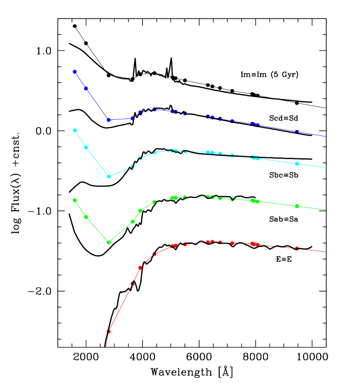
Figure 7: The SED for template galaxy models (connected solid dots) is compared with “mean” empirical spectra along the Hubble morphological sequence (thick solid line). Data for types E (the M81 case), Sbc, Scd, and Im are from Coleman et al. (1980), while the Sab case is from Pence (1976). Empirical and theoretical templates are matched as labeled on each plot.

A comparison of our output with the empirical SED for template galaxies along the Hubble sequence is carried out in Fig. 7. Mean reference spectra are those assembled by Coleman et al. (1980) for types E (the M81 case), Sbc, Scd, and Im, while the SED of the Sab type in the figure is from Pence (1976). From the plots one can appreciate a fully suitable match between observed and theoretical SED longward of the $U$ band. Two interesting features, however, are worth of attention, to a deeper analysis: i) empirical templates (especially for spirals) always display a “depressed” ultraviolet emission, compared to the theoretical SED; ii) the Im empirical template more closely fits a young ($\sim 5$ Gyr) theoretical model.

As we have further discussed in Paper I, point i) is the obvious signature of dust in the SED of real galaxies. Although this effect is not explicitely taken into account in our models, it could easily be assessed in any ex-post analysis of the observations by adopting a preferred shape for the attenuation curve to correct the data, like proposed, for example, by the studies of Calzetti (1999) and Bruzual et al. (1988). In any case, as we were previously mentioning, it is evident from Fig. 7 that dust effects only enter at the very short wavelength range ($\lambda\la 3000$ Å) of galaxy SED. Finally, as for point ii) above, one has to recall that the Coleman et al. reference template for the Im type relies on just one “extremely bue irregular galaxy” (i.e. NGC 4449). For this target, authors report, as integrated colors, $(U-V)=-0.06$ and $(B-V)=0.32$, placing the object at the extreme blue range of the typical colors for irregulars (see, for instance, Fig. 3 and 4, and also the relevant discussion by Fukugita et al., 1995); a younger age is therefore required to match the observed SED for this galaxy.

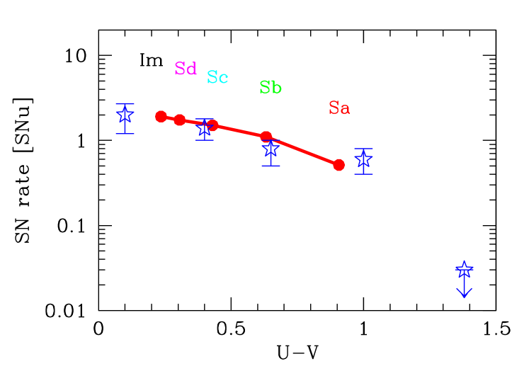
Figure 8: Theoretical SN(II+Ibc) rates, singled out from eqs. (10) and (8) (solid line and dots) are compared with the empirical estimates of Cappellaro et al. (1999) (star markers) from their survey of over 10 000 low-redshift galaxies. The $U-V$ refers to the galaxy integrated color (corrected for reddening in case of observations).

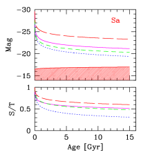
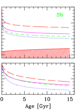
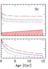
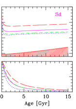
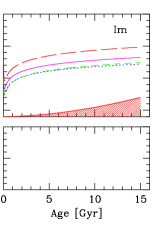
Figure 9: Upper plots in each panel: theoretical luminosity evolution for late-type galaxy models. A total stellar mass $M_{gal}=10^{11}~{}M_{\odot}$ is assumed at 15 Gyr. Solid lines track bolometric magnitude, while dotted lines are for the $U$ band, short-dashed for $V$, and long-dashed for the $K$ band. The shaded area in each plot sketches (in arbitrary linear scale) the evolution of $M_{gal}$ according to star formation history for each morphological type.
Lower plots in each panel: the corresponding evolution of the morhological parameter S/T in the bolometric, $U,V$, and $K$ bands (same line caption as in the upper panels). Note that S/T $\to 1$ at early epochs (excepting the Im model) due to the increasing bulge contribution.

4.1 Supernova and Hypernova rates

A natural output of template models deals with the current formation rate of core-collapsed stellar objects. This includes types II/Ibc Supernovae and their Hypernova (HN) variant (Paczyński, 1998) for very high-mass stars. Both the SN and HN events are believed to generate from the explosion of single massive stars and have therefore a direct link with the galaxy stellar birthrate. Hypernovae, in particular, have recently raised to a central issue in the investigation of the extragalactic Gamma-ray bursts (Nakamura et al., 2000; Woosley & MacFayden, 2000).

If we assume, with Bressan et al. (1994), that all stars with $M_{*}\geq 5~{}M_{\odot}$ eventually undergo an explosive stage, and those more massive than $40~{}M_{\odot}$ generate a Hypernova burst (Iwamoto et al., 1998), then the number of SN(II+Ibc)+HN events in a SSP of total mass $M_{\rm SSP}$ (in solar units) and Salpeter IMF can be written as:

$$N_{\rm SN+HN} = {0.35\over 1.35}\,\left[{{5^{-1.35}-120^{-1.35}}\over{0.1^{-0.35}-120^{-0.35}}}\right]\,M_{\rm SSP}$$ (7)

$$= 0.0142\,M_{\rm SSP}\quad[M_{\odot}^{-1}].$$

The expected fraction of SN(II+Ibc) relative to HN candidates, for a Salpeter IMF, derives as

$$[N_{\rm SN}:N_{\rm HN}]=[20:1].$$ (8)

If disk SFR does not change much on a timescale comparable with lifetime of $5~{}M_{\odot}$ stars (i.e. $\sim 10^{8}$ yrs), then a simplified approach is allowed for composite stellar populations. From eq. (2), at 15 Gyr we have that ${\rm SFR}_{o}=b\,\langle{\rm SFR}\rangle=b\,{\rm M}_{\rm disk}/(15\times 10^{9}{\rm yr})$, and the current SN+HN event rate, $R_{\rm SN+HN}=dN_{\rm SN+HN}/dt$ can therefore be written as

$$R_{\rm SN+HN}=0.0142~{}{\rm SFR}_{o}=0.0142\,b\,f\,{{M_{\rm gal}}\over{(15\times 10^{9}{\rm yr})}},$$ (9)

being $f$ the stellar mass fraction of disk (see Table 3). We could more suitably arrange eq. (9) in terms of bolometric mass-to-light ratio and total $B$ luminosity of the parent galaxy (again, cf. Table 3 for the reference quantities). With little arithmetic, $R_{\rm SN+HN}$ eventually becomes

$$R_{\rm SN+HN}=0.95\,b\,f\left({M\over L_{\rm bol}}\right)\,10^{-0.4({\rm Bol-B}+0.69)}\,L_{10}^{\rm B}.$$ (10)

In the equation, $L_{10}^{\rm B}$ is the galaxy $B$ luminosity in unit of $10^{10}L_{\odot}^{\rm B}$, while $(Bol-B)$ is the galaxy bolometric correction to the Johnson $B$ band, derived from Tables 8-12 as $(Bol-B)=(Bol-V)-(B-V)$. With this notation, eq. (10) directly provides the SN+HN rate in the usual SNu units [i.e. 1 SNu = 1 SN(100yr)^-1($10^{10}L_{\odot}^{\rm B})^{-1}$].

Table 4: Theoretical SN (II+Ibc) and Hypernova rates for late-type galaxies at present time

Hubble	SN+HN(a)	HN(a)	$\tau_{SN+HN}^{(b)}$	$\tau_{HN}^{(b)}$
Type	[SNu]	[SNu]	[yr]	[yr]
Sa	0.52	0.025	194	4100
Sb	1.10	0.052	91	1900
Sc	1.50	0.071	67	1400
Sd	1.74	0.082	58	1250
Im	1.91	0.090	52	1100

^(a)SN(II+Ibc)+HN and HN rates, in SNu units.
^(b)Expected timescale between two SN or HN events in a $10^{11}~{}M_{\odot}$ galaxy

Table 4 summarizes our results for late-type galaxies. In addition to the theoretical event rate, we also reported in the table the typical timescale elapsed between two SN and HN bursts in a $10^{11}~{}M_{\odot}$ galaxy. As $R_{\rm SN+HN}$ tightly depends on SFR, it should correlate with galaxy ultraviolet colors; this is shown in Fig. 8, where a nice agreement is found with the empirical SN rates from the recent low-redshift galaxy survey by Cappellaro et al. (1999).

4.2 Back-in-time evolution

Theoretical luminosity evolution for disk-dominated systems in the Johnson $U,V$, $K$ bands, and for the bolometric is displayed in the upper panels of Fig. 9; to each plot we also added a shaded curve that traces the value of $M_{\rm gal}$ vs. time. Lower panels in the figure represent the expected evolution of the morphological parameter S/T for the same photometric bands. One striking feature in the Sa-Sd plots is the increasing luminosity contribution of the bulge at early epochs ($L_{\rm bulge}\propto t^{-0.8}$ in bolometric, see Table 1). This greatly compensates the drop in disk luminosity ($L_{\rm disk}\propto t\,L_{\rm bulge}$, from eq. 1, for a constant SFR), and acts in the sense of predicting more nucleated (S/T $\to 1$) galaxies at high redshift compared with present-day (i.e. 15 Gyr) objects.

This effect is shown in Fig. 10, where we track back-in-time evolution of the morphology parameter S/T in the ultraviolet range (Johnson $U$ band). Due to bulge enhancement, one sees that later-type spirals (Sc-Sd types) at 1 Gyr closely resemble present-day S0-Sa systems.

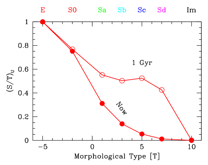
Figure 10: Inferred evolution of the $U$-band morphological parameter S/T for galaxies along the Hubble sequence. Bulge enhancement at early epochs leads later-type systems (Sc-Sd types) at 1 Gyr to closely resemble present-day S0-Sa galaxies.

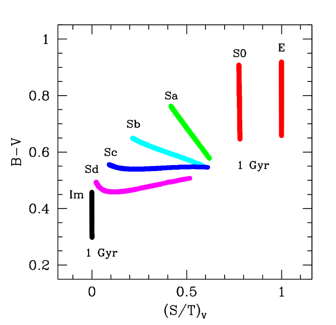
Figure 11: Restframe $B-V$ color evolution, from 15 to 1 Gyr, vs. $V$-band morphological parameter S/T for galaxy models along the Hubble sequence. The increasing luminosity contribution of the bulge component back in time makes spiral galaxies at high redshift more nucleated than present-day homologues. For high-redshift observations this induces a bias toward both “spiked” and irregular systems with increasing distances (consider the x-axis projection of the figure) and conspires against the detection of grand-design spirals.

A color vs. S/T plot, like in Fig. 11, effectively summarizes overall galaxy properties at the different ages. Color evolution is much shallower for spirals than for ellipticals and, as expected, the trend is always in the sense of having bluer galaxies at earlier epochs (excepting perhaps Sd spirals) independently of the star formation details. Restframe colors tend however to “degenerate” with primeval late-type galaxies approaching the E model at early epochs as a consequence of the bulge brightening.

If one does not mind evolution, all these effects could lead to a strongly biased interpretation of high-redshift observations. For example, by relying on galaxy apparent colors (that is by reading Fig. 11 from the y-axis, with no hints about morphology), the high-redshift galaxy population might show a lack of (intrinsically) red objects (ellipticals?), and enhance on the contrary blue galaxies (spirals?). On the other hand, if we account for apparent morphology alone (that is by reading Fig. 11 from the x-axis), then a bimodal excess of bulge-dominated systems (S/T $\to 1$) and irregular star-forming galaxies (S/T $\sim 0$) would appear at large distances (van den Bergh et al., 2000; Kajisawa & Yamada, 2001). In fact, fiducial Im systems would eventually dominate with increasing redshift due to the disfavoring effect of k-correction on ellipticals, at least in the optical range. Among others, this should also conspire against the detection of grand-design spirals in high-redshift surveys (e.g. van den Bergh et al., 1996).

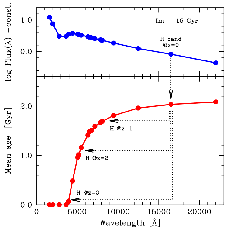
Figure 12: Theoretical SED for the 15 Gyr Im galaxy model (upper panel), and “mean” age, $\overline{t}_{*}$, of the prevailing stars in the different photometric bands, according to eq. (12) (lower panel). Note that younger (and more massive) stars contribute, in average, to global luminosity at shorter wavelength. Assuming to observe this galaxy in the infrared H band at increasing distances (namely, from $z=0$ to 3, as labeled), one might be noticing an apparent increase in the fresh star-formation activity with redshift (and a correspondingly younger inferred age) just as a consequence of probing blue/ultraviolet emission in the galaxy restframe.

4.3 Redshift and age bias

The effect of redshift, and its induced selective sampling of galaxy stellar population with changing wavelength, has even more pervasive consequences, as far as we track evolution of star-forming systems at increasing distances.

According to eq. (1), the mean luminosity-weighted age of stars contributing to galaxy luminosity can be written as

$$\overline{t}_{*}={{\int_{0}^{t}\tau\ L_{\rm SSP}(\tau){\it SFR}(t-\tau)\ d\tau}\over{L_{\rm tot}(t)}}.$$ (11)

The “representative” age of stars changes therefore across galaxy SED, since $L_{\rm SSP}\propto t^{-\alpha}$, and $\alpha$ depends on wavelength (cf. Table 1). As, in our parameterization, SFR $\propto t^{-\eta}$, then eq. (11) becomes

$$\overline{t}_{*}={{\int_{0}^{t}\tau^{1-\alpha}\ (t-\tau)^{-\eta}\ d\tau}\over{\int_{0}^{t}\tau^{-\alpha}\ (t-\tau)^{-\eta}\ d\tau}}={{1-\alpha}\over{2-\alpha-\eta}}\ t.$$ (12)

In bolometric, $\alpha\simeq 0.8$ that is, for a constant SFR, $\overline{t}_{*}\simeq 0.2\,t$: at 15 Gyr, bright stars are therefore in average $\sim 3~{}$Gyr old. As an instructive example, in Fig. 12 we displayed the mean age of stars contributing to galaxy luminosity at different wavelength for our 15 Gyr Im template model. Note that the value of $\overline{t}_{*}$ smoothly decreases at shorter wavelength, reaching a cutoff about 4000 Å, when $\alpha$ exceeds unity and $\overline{t}_{*}$ coincides with the lifetime of the highest-mass stars in the IMF (see Paper I for the important consequences of this feature on galaxy ultraviolet SED). As a consequence, when tracking redshift evolution of star-forming galaxies through a given optical/infrared photometric band, one would be left with the tricky effect that distant objects appear to be younger than local homologues in spite of any intrinsic evolution.

5 Luminosity contribution from residual gas

In addition to the prevailing role of stars, a little fraction of galaxy luminosity (especially in late-type systems) is provided also by residual gas. Its contribution is both in terms of continuum emission, mainly from free-bound $e^{-}$ transitions in the H II regions, and emission-line enhancement. This is the typical case of the Balmer series, for instance, but also some forbidden lines, like those of [O II] at 3727 Å and [O III] at 5007 Å, usually appear as a striking feature in the galaxy spectrum (Kennicutt, 1992; Sodré & Stasinska, 1999).

The key triggering process for gas luminosity is the ultraviolet emission from short-living ($t\la 10^{7}$ yrs) stars of high mass ($M_{*}\ga 10~{}M_{\odot}$), that supply most of the ionizing Lyman photons in the H II regions. The presence of emission lines is, in this sense, the most direct probe of ongoing star formation in a galaxy. If gas is optically thin and tracks the distribution of young stars, then one could expect a tight relationship between the actual SFR (via the number of UV-emitting stars) and the strength of the Hydrogen emission lines.

For its complexity, a detailed treatment of the nebular emission is obviously beyond the scope of this paper (see, e.g., Stasińka, 2000 and Magris et al., 2003, for a reference discussion on this subject). Here, we are rather interested in exploring the general trend of some relevant features, like the Balmer emission lines, that could supply an effective tool for the SFR diagnostics when compared with the observations.

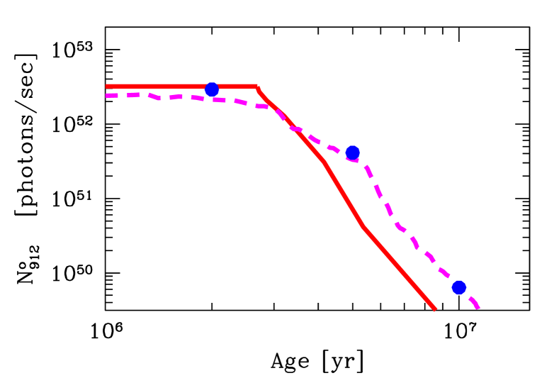
Figure 13: The expected rate of Lyman photons, $N_{912}^{o}$, for a Salpeter SSP of $10^{6}~{}M_{\odot}$ with stars in the range 0.1-120 $M_{\odot}$. Our results (thick solid line) consistently compare with the starburst models of Leitherer et al. (1999) (dashed line), and Mas-Hesse & Kunth (1991) (solid dots). Both these models have been rescaled to our output by matching the number of stars between 60 and $100~{}M_{\odot}$.

5.1 Nebular emission

Our approach is similar to that of Leitherer & Heckman (1995), adopting for the gas standard physical conditions, with $T=10\,000$ K and $Y=0.28$ for Helium abundance (in mass). We will assume a full opacity to Lyman photons so that, once the photon rate $N_{912}^{o}$ from high-mass stars can be set from the detailed synthesis model, nebular continuum derives as

$$L_{gas}(\lambda)={c\over{\lambda^{2}}}{\gamma_{\lambda}\over\alpha_{B}}~{}N_{912}^{o}.$$ (13)

In the equation, $\gamma(\lambda)$ is the continuum emission coefficient for the H-He chemical mix, according to Aller (1984), and includes both free-free and bound-free transitions by Hydrogen and neutral Helium, as well as the two-photons continuum of Hydrogen. The Hydrogen recombination coefficient (according to Case B of Baker and Menzel 1938) is from Osterbrok (1974) and has been set to $\alpha_{B}=2.59~{}10^{-13}$ cm³ s^-1.

According to eq. (13), the nebular continuum directly scales with $N_{912}^{o}$ so that, as a relevant output of our models, in Fig. 13 we computed the expected rate of $\lambda<912$ Å photons for a Salpeter SSP with upper cutoff mass at 120 $M_{\odot}$. Our results compare consistently with the starburst models of Leitherer et al. (1999), and Mas-Hesse & Kunth (1991). To account for different IMF slope and/or stellar mass limits, comparison is made by matching our number of stars between 60 and $100~{}M_{\odot}$ in a $10^{6}\ M_{\odot}$ SSP. The agreement between the models is fairly good, with a tendency of our SSP, however, to evolve faster given a slightly shorter lifetime assumed for high-mass stars (cf. Paper I for more details on the adopted stellar clock).

Table 5: Balmer-line intensities for late-type galaxy templates^(a)

Age		Sa					Sb					Sc
[Gyr]		$H\delta$	$H\gamma$	$H\beta$	$H\alpha$		$H\delta$	$H\gamma$	$H\beta$	$H\alpha$		$H\delta$	$H\gamma$	$H\beta$	$H\alpha$
1.0		0.55	1.63	4.11	13.8		0.79	2.33	6.01	20.6		0.88	2.59	6.73	23.1
1.5		0.56	1.63	4.05	13.3		0.84	2.49	6.35	21.4		1.03	3.02	7.86	26.9
2.0		0.56	1.64	4.00	13.0		0.88	2.58	6.55	21.9		1.12	3.29	8.56	29.3
3.0		0.56	1.64	3.93	12.4		0.91	2.69	6.76	22.3		1.22	3.58	9.36	32.1
4.0		0.56	1.64	3.87	12.1		0.93	2.75	6.87	22.5		1.27	3.73	9.76	33.5
5.0		0.56	1.64	3.83	11.8		0.95	2.79	6.92	22.5		1.29	3.80	9.97	34.2
6.0		0.56	1.64	3.79	11.6		0.95	2.81	6.95	22.5		1.31	3.84	10.1	34.5
8.0		0.55	1.63	3.73	11.2		0.96	2.83	6.96	22.3		1.31	3.87	10.1	34.6
10.0		0.55	1.63	3.68	10.9		0.97	2.84	6.95	22.1		1.31	3.86	10.1	34.3
12.5		0.55	1.62	3.62	10.6		0.97	2.85	6.92	21.9		1.30	3.84	9.98	33.9
15.0		0.55	1.62	3.58	10.4		0.97	2.84	6.88	21.6		1.29	3.80	9.85	33.3
Age		Sd					Im
[Gyr]		$H\delta$	$H\gamma$	$H\beta$	$H\alpha$		$H\delta$	$H\gamma$	$H\beta$	$H\alpha$
1.0		1.20	3.54	9.46	33.4		2.62	7.71	24.0	99.9
1.5		1.43	4.20	11.4	40.7		2.42	7.13	21.9	90.1
2.0		1.54	4.54	12.5	45.0		2.29	6.76	20.5	83.2
3.0		1.63	4.81	13.3	48.6		2.13	6.28	18.7	74.6
4.0		1.65	4.87	13.5	49.5		2.03	5.98	17.6	69.2
5.0		1.65	4.86	13.5	49.4		1.95	5.76	16.8	65.3
6.0		1.64	4.82	13.4	48.8		1.90	5.59	16.2	62.3
8.0		1.60	4.72	13.0	47.4		1.81	5.34	15.3	57.9
10.0		1.57	4.64	12.7	45.9		1.75	5.15	14.6	54.6
12.5		1.54	4.52	12.3	44.2		1.69	4.97	14.0	51.6
15.0		1.50	4.43	12.0	42.7		1.64	4.84	13.5	49.4

^(a)The listed quantity is the Balmer emission-line equivalent width in Å.

5.2 Balmer emission-line evolution

The equivalent width of Balmer lines has been derived via the $H\beta$ luminosity, defined as

$$L(H\beta)=h\nu_{H\beta}\ {{\alpha_{H\beta}}\over{\alpha_{B}}}\ N_{912}^{o}.$$ (14)

For the effective recombination coefficient at $T=10\,000$ K we adopted the value $\alpha_{H\beta}=3.03~{}10^{-14}$ cm³ s^-1 from Osterbrok (1974). This eventually leads to a calibration for the $H\beta$ luminosity such as

$$L(H\beta)=4.78~{}10^{-13}\ N_{912}^{o}~{}~{}~{}~{}[{\rm erg~{}s}^{-1}].$$ (15)

This result agrees within a 0.4% both with the Leitherer & Heckman (1995) and Copetti et al. (1986) calculations. Balmer-line intensities, relative to $H\beta$, are from Osterbrok (1974, Table 4.2 therein) for the relevant value of the temperature.

If the continuum (including both the contribution from stars and gas, $L_{*}$ and $L_{\rm gas}$, respectively) is assumed to vary slowly with wavelength, adjacent to the line, then the $H\beta$ equivalent width can be written as

$$W(H\beta)={{L(H\beta)}\over{(L_{*}+L_{gas})}}$$ (16)

and all the other lines derive accordingly. The computed value of $W(H\beta)$ should be regarded of course as the net emission from the gas component (that is after correcting the spectral feature for stellar absorption).

In Table 5 we report our final results, also summarized in Fig. 14. The upper panel of the figure displays the Balmer-line evolution for each of our template galaxy. As expected, $H\alpha$ is the dominating feature, while gas emission sensibly decreases for $H\gamma$ and $H\delta$. In addition, the onset of the galaxy bulge at early epochs works in the sense of decreasing line emission because of the “diluiting” factor $L_{*}$ in eq. (16) (cf. for example the diverging path of Im and Sd evolution in Fig. 14).

In the lower panel of the same figure we computed the fraction $L_{\rm gas}/(L_{*}+L_{\rm gas})$ supplied by the nebular emission to the galaxy continuum at different wavelength, between 4100 and 6600 Å, evaluated close to each Balmer line. As far as the galaxy broad-band colors are concerned, we see that nebular luminosity is almost negligible in our age range, and contributes at most by a few percent to the galaxy total luminosity.

One striking feature that stems from the analysis of Fig. 14 is the relative insensitivity of Balmer-line equivalent width to time. This is somewhat a consequence of the birthrate law assumed in our models. Actually, for the case of $H\beta$, like in eq. (16) for instance, we have that $L(H\beta)$ mainly responds to SFR_o, through the selective contribution of hot stars of high mass, while the contiguous spectral continuum collects a much more composite piece of information from all stars (and it is, roughly, $L_{*}\propto\langle{\rm SFR}\rangle$); this makes $W(H\beta)$ better related to $b$. In our framework, we could therefore conclude that observation of Balmer emissions certainly provides important clues to size up the actual star formation activity in a galaxy, but it will barely constrain age.

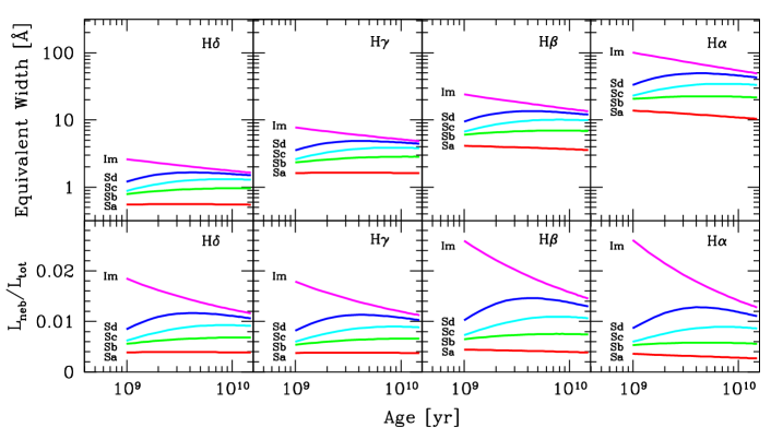
Figure 14: Expected evolution for Balmer emission and nebular luminosity from residual gas in our late-type galaxy templates. Upper panel displays the equivalent width of each Balmer feature along galaxy age. Lower panel is the fraction of nebular luminosity supplied to the total galaxy continuum evaluated at the relevant wavelength close to each Balmer line.

6 Summary and conclusions

In this work we attempted a comprehensive analysis of some relevant aspects of galaxy photometric evolution. Colors and basic morphological features for early- and late-type systems have been reproduced by means of a set of theoretical population synthesis models, that evaluate the individual photometric contribution of the three main stellar components of a galaxy, namely the bulge, disk and halo.

Facing the formidable complexity of the problem (and the lack, to our present knowledge, of any straightforward “prime principle” governing the galaxy evolution), we chose to adopt a “heuristic” point of view, where the distinctive properties of present-day galaxies derive from a minimal set of physical assumptions and are mainly constrained by the observed colors along the Hubble sequence.

One important feature of our models is that galaxy SFR is a natural output of the gas-to-star conversion efficiency, that we assume to be an intrinsic and distinctive feature of galaxy morphological type (see eq. 2). Our treatment of the star vs. gas interplay is therefore somewhat different from other popular approaches, that rely on the Schmidt law.

Our results show that star formation history, as a function of the overall disk composition along the late-type galaxy sequence, appears to be a main factor to modulate galaxy photometric properties. In general, the disk photometric contribution is the prevailing one in the luminosity (but not necessarily in the mass…) budget of present-day galaxies. Table 3 shows, for instance, that well less than a half of the total mass of a Sbc galaxy like the Milky Way is stored in the disk stars, while the latter provide over 3/4 of the global luminosity.

As shown in Fig. 4, the observed colors of present-day galaxies tightly constrain the stellar birthrate leading to a smooth increasing trend for $b$ from E to Im types (cf. Table 2 and also Fig. 8 in Paper I).

The comparison with observed SN rate is an immediate “acid test” for our models, due to the marked sensitivity of this parameter to the current SFR. The remarkably tuned match of our theoretical output with the SN observations in low-redshift galaxies (cf. Fig. 8) is, in this regard, extremely encouraging. As a possibly interesting feature for future observational feedback, we give in Table 4 also a prediction of the Hypernova event rate in late-type galaxies; this quite new class of stars is raising an increasing interest for its claimed relationship with the Gamma-ray bursts and the possible relevant impact of these events in the cosmological studies.

Another important point of our theoretical framework deals with the fact that galaxy evolution is tracked in terms of the individual history of the different galaxy sub-systems. This is a non-negligible aspect, as diverging evolutionary paths are envisaged for the bulge vs. disk stellar populations. As discussed in Sec. 4.2, if $L_{\rm bulge}\propto t^{-0.8}$ in bolometric, and $L_{\rm disk}\propto t\,L_{\rm bulge}$, then one has to expect that $L_{\rm bulge}/L_{\rm disk}\propto t^{-1}$, that is the bulge always ends up as the dominant contributor to galaxy luminosity at early epochs.

As a consequence, the current morphological look of galaxies might drastically change when moving to larger distances, and we have shown in Sec. 4 how sensibly this bias could affect the observation (and the interpretation) of high-redshift surveys.

In addition to broad-band colors, we have also briefly assessed the photometric contribution of the nebular gas, studying in particular the expected evolution of Balmer line emission in disk-dominated systems. As a main point in our analysis, models show that striking emission lines, like $H\alpha$, can very effectively track stellar birthrate in a galaxy. For these features to be useful age tracers as well, however, one should first assess how $b$ could really change with time on the basis of supplementary (and physically independent) arguments.

As a further follow-up of this work, we finally plan to complete the analysis of these galaxy template models providing, in a future paper, also the evolutionary $k$ corrections and other reference quantities for a wider application of the model output to high-redshift studies.

Appendix A Synthetic photometry for template galaxy models

We report, in the series of Tables 6-12, the detailed output of the template galaxy models for the different Hubble morphological types. All the models assume a total stellar mass $M_{\rm gal}=(M_{\rm bulge}+M_{\rm disk}+M_{\rm halo})=10^{11}~{}M_{\odot}$ at 15 Gyr (see Footnote 6 for an operational definition of $M_{\rm gal}$).

Full details on the photometric systems (i.e. band wavelength and magnitude zero points) can be obtained from Table 1.

Each table is arranged in two blocks of data; caption for entries in the upper block is the following:
Column 1 - Age of the galaxy, in Gyr;
Column 2 - Absolute magnitude of the model, in bolometric. For the Sun, we assume $Bol_{\odot}=4.72$;
Column 3 - Bolometric correction to the Johnson $V$ band. The adopted solar value is $(Bol-V)_{\odot}=-0.07$;
Column 4 to 10 - Integrated broad-band colors in the Johnson system (filters $U,B,V,R,I,J,H,K$);
Lower block of data has the following entries:
Column 1 - Age of the galaxy, in Gyr;
Column 2 to 3 - Integrated colors in the Johnson/Cousins system (filters $R_{c}$ and $I_{c}$);
Column 4 to 6 - Integrated colors in the Gunn system (filters $g,r,i$), with the $g-V$ color allowing a self-consistent link to the Johnson photometry;
Column 7 to 10 - Integrated colors in the Washington system (filters $C,M,T_{1},T_{2}$), with the $M-V$ color linking the Johnson photometry.

It may also be worth recalling that a straightforward transformation of our photometry to the Sloan SDSS photometric system (extensively used in recent extragalactic studies) can be carried out according to the equations set of Fukugita et al. (1996, their eq. 23).

To allow an easier graphical display and interpolation of the data, all the magnitudes and colors in Tables 6-12 are reported with a three-digit nominal precision; see, however, Sec. 2 and 4 for a more detailed discussion of the real internal uncertainty of synthetic photometry in our models.

The entire theoretical database is publicly available at the author’s Web site: http://www.bo.astro.it/$\sim$eps/home.html.

Table 6: Template model for E galaxies

		Johnson
Age [Gyr]	Bol	Bol–V	U–V	B–V	V–R	V–I	V–J	V–H	V–K
1.0	–23.100	–0.722	0.740	0.656	0.698	1.301	1.916	2.630	2.821
1.5	–22.736	–0.745	0.840	0.696	0.725	1.343	1.968	2.688	2.882
2.0	–22.493	–0.764	0.907	0.723	0.744	1.371	2.004	2.727	2.923
3.0	–22.142	–0.792	1.003	0.763	0.771	1.413	2.055	2.783	2.983
4.0	–21.888	–0.814	1.073	0.791	0.791	1.443	2.093	2.824	3.027
5.0	–21.698	–0.832	1.125	0.813	0.806	1.465	2.121	2.855	3.059
6.0	–21.543	–0.847	1.168	0.830	0.818	1.484	2.144	2.880	3.086
8.0	–21.298	–0.870	1.235	0.858	0.837	1.513	2.181	2.920	3.128
10.0	–21.106	–0.890	1.287	0.880	0.852	1.536	2.209	2.952	3.162
12.5	–20.919	–0.909	1.338	0.902	0.867	1.559	2.237	2.983	3.194
15.0	–20.764	–0.925	1.381	0.919	0.879	1.577	2.260	3.008	3.221
	Cousins		Gunn			Washington
Age [Gyr]	V–Rc	V–Ic	g–V	g–r	g–i	C–M	M–V	M–T1	M–T2
1.0	0.488	1.018	0.154	0.251	0.417	0.494	0.230	0.639	1.223
1.5	0.508	1.050	0.163	0.282	0.460	0.551	0.242	0.667	1.269
2.0	0.522	1.072	0.169	0.303	0.489	0.590	0.250	0.686	1.300
3.0	0.542	1.105	0.178	0.334	0.531	0.645	0.262	0.714	1.345
4.0	0.556	1.128	0.184	0.356	0.562	0.685	0.271	0.734	1.378
5.0	0.567	1.145	0.189	0.373	0.585	0.715	0.277	0.749	1.402
6.0	0.576	1.160	0.193	0.386	0.604	0.740	0.283	0.762	1.422
8.0	0.590	1.182	0.200	0.408	0.634	0.779	0.291	0.781	1.454
10.0	0.601	1.200	0.204	0.425	0.658	0.809	0.298	0.797	1.479
12.5	0.612	1.218	0.209	0.442	0.681	0.839	0.304	0.812	1.504
15.0	0.621	1.232	0.213	0.456	0.700	0.864	0.310	0.824	1.524

Table 7: Template model for S0 galaxies

		Johnson
Age [Gyr]	Bol	Bol–V	U–V	B–V	V–R	V–I	V–J	V–H	V–K
1.0	–23.146	–0.699	0.710	0.644	0.686	1.277	1.881	2.584	2.769
1.5	–22.782	–0.721	0.807	0.684	0.714	1.320	1.934	2.642	2.830
2.0	–22.539	–0.738	0.872	0.711	0.733	1.348	1.969	2.681	2.871
3.0	–22.188	–0.766	0.966	0.751	0.760	1.390	2.021	2.738	2.931
4.0	–21.934	–0.787	1.034	0.779	0.780	1.420	2.058	2.779	2.975
5.0	–21.744	–0.804	1.085	0.801	0.795	1.442	2.086	2.810	3.007
6.0	–21.589	–0.818	1.126	0.818	0.807	1.461	2.109	2.835	3.034
8.0	–21.344	–0.841	1.192	0.846	0.826	1.490	2.146	2.875	3.077
10.0	–21.152	–0.859	1.243	0.868	0.841	1.513	2.175	2.906	3.110
12.5	–20.964	–0.878	1.293	0.890	0.856	1.536	2.203	2.937	3.142
15.0	–20.809	–0.893	1.334	0.908	0.868	1.554	2.226	2.963	3.169
	Cousins		Gunn			Washington
Age [Gyr]	V–Rc	V–Ic	g–V	g–r	g–i	C–M	M–V	M–T1	M–T2
1.0	0.480	1.000	0.152	0.239	0.398	0.471	0.226	0.629	1.204
1.5	0.500	1.033	0.161	0.270	0.441	0.526	0.239	0.657	1.250
2.0	0.514	1.055	0.167	0.291	0.470	0.564	0.247	0.676	1.281
3.0	0.534	1.087	0.176	0.322	0.513	0.618	0.259	0.704	1.326
4.0	0.548	1.110	0.182	0.344	0.543	0.657	0.268	0.724	1.359
5.0	0.559	1.128	0.187	0.361	0.567	0.686	0.274	0.740	1.383
6.0	0.568	1.142	0.191	0.375	0.586	0.711	0.279	0.752	1.403
8.0	0.582	1.165	0.197	0.397	0.616	0.749	0.288	0.772	1.435
10.0	0.593	1.182	0.202	0.414	0.639	0.778	0.295	0.787	1.460
12.5	0.604	1.200	0.207	0.430	0.662	0.808	0.301	0.802	1.485
15.0	0.613	1.214	0.211	0.444	0.682	0.832	0.307	0.815	1.505

Table 8: Template model for Sa galaxies

		Johnson
Age [Gyr]	Bol	Bol–V	U–V	B–V	V–R	V–I	V–J	V–H	V–K
1.0	–23.221	–0.737	0.530	0.576	0.649	1.220	1.809	2.504	2.683
1.5	–22.895	–0.750	0.594	0.605	0.671	1.253	1.850	2.548	2.730
2.0	–22.678	–0.760	0.636	0.625	0.685	1.275	1.877	2.578	2.761
3.0	–22.365	–0.776	0.695	0.653	0.706	1.307	1.917	2.620	2.806
4.0	–22.140	–0.788	0.736	0.674	0.722	1.330	1.946	2.651	2.838
5.0	–21.972	–0.798	0.766	0.689	0.733	1.348	1.967	2.674	2.862
6.0	–21.835	–0.806	0.790	0.701	0.743	1.362	1.984	2.693	2.882
8.0	–21.620	–0.820	0.827	0.720	0.757	1.384	2.012	2.723	2.913
10.0	–21.452	–0.831	0.856	0.735	0.769	1.402	2.034	2.746	2.938
12.5	–21.288	–0.841	0.884	0.750	0.780	1.419	2.055	2.769	2.962
15.0	–21.153	–0.850	0.907	0.762	0.790	1.433	2.073	2.788	2.982
	Cousins		Gunn			Washington
Age [Gyr]	V–Rc	V–Ic	g–V	g–r	g–i	C–M	M–V	M–T1	M–T2
1.0	0.451	0.954	0.138	0.194	0.338	0.365	0.208	0.588	1.139
1.5	0.467	0.979	0.145	0.219	0.372	0.402	0.217	0.610	1.175
2.0	0.478	0.996	0.150	0.235	0.394	0.427	0.224	0.624	1.199
3.0	0.493	1.021	0.157	0.259	0.427	0.462	0.233	0.646	1.234
4.0	0.505	1.038	0.161	0.276	0.451	0.486	0.239	0.661	1.259
5.0	0.513	1.052	0.165	0.289	0.468	0.503	0.244	0.672	1.278
6.0	0.520	1.062	0.168	0.299	0.483	0.518	0.248	0.682	1.293
8.0	0.530	1.080	0.173	0.315	0.506	0.541	0.254	0.696	1.317
10.0	0.539	1.093	0.176	0.328	0.523	0.558	0.259	0.708	1.336
12.5	0.547	1.106	0.180	0.341	0.541	0.575	0.264	0.719	1.355
15.0	0.554	1.117	0.183	0.351	0.555	0.588	0.268	0.728	1.370

Table 9: Template model for Sb galaxies

		Johnson
Age [Gyr]	Bol	Bol–V	U–V	B–V	V–R	V–I	V–J	V–H	V–K
1.0	–23.114	–0.757	0.467	0.551	0.635	1.199	1.784	2.477	2.655
1.5	–22.842	–0.770	0.501	0.568	0.649	1.221	1.810	2.504	2.683
2.0	–22.667	–0.778	0.521	0.579	0.658	1.234	1.826	2.520	2.700
3.0	–22.422	–0.790	0.546	0.594	0.671	1.252	1.848	2.542	2.722
4.0	–22.252	–0.797	0.562	0.604	0.679	1.265	1.863	2.557	2.737
5.0	–22.128	–0.802	0.573	0.611	0.686	1.274	1.874	2.568	2.749
6.0	–22.030	–0.806	0.583	0.617	0.691	1.282	1.883	2.577	2.758
8.0	–21.878	–0.812	0.597	0.627	0.699	1.294	1.897	2.592	2.772
10.0	–21.763	–0.817	0.609	0.634	0.706	1.303	1.908	2.603	2.784
12.5	–21.653	–0.821	0.621	0.642	0.713	1.313	1.920	2.615	2.796
15.0	–21.565	–0.824	0.632	0.649	0.718	1.321	1.929	2.624	2.806
	Cousins		Gunn			Washington
Age [Gyr]	V–Rc	V–Ic	g–V	g–r	g–i	C–M	M–V	M–T1	M–T2
1.0	0.441	0.937	0.133	0.178	0.316	0.328	0.201	0.573	1.116
1.5	0.451	0.953	0.138	0.194	0.338	0.347	0.207	0.587	1.139
2.0	0.458	0.963	0.141	0.204	0.351	0.359	0.211	0.596	1.154
3.0	0.467	0.977	0.144	0.217	0.370	0.373	0.216	0.608	1.174
4.0	0.473	0.986	0.147	0.227	0.383	0.382	0.220	0.616	1.188
5.0	0.478	0.993	0.149	0.234	0.393	0.388	0.222	0.622	1.198
6.0	0.481	0.999	0.151	0.239	0.401	0.394	0.224	0.627	1.206
8.0	0.487	1.008	0.153	0.248	0.413	0.402	0.228	0.635	1.219
10.0	0.492	1.015	0.155	0.256	0.423	0.409	0.231	0.642	1.230
12.5	0.497	1.022	0.157	0.263	0.433	0.417	0.233	0.648	1.240
15.0	0.501	1.029	0.159	0.269	0.442	0.423	0.236	0.653	1.249

Table 10: Template model for Sc galaxies

		Johnson
Age [Gyr]	Bol	Bol–V	U–V	B–V	V–R	V–I	V–J	V–H	V–K
1.0	–22.799	–0.770	0.453	0.546	0.633	1.199	1.786	2.480	2.659
1.5	–22.594	–0.788	0.449	0.547	0.638	1.204	1.791	2.484	2.662
2.0	–22.478	–0.798	0.441	0.546	0.639	1.205	1.790	2.481	2.658
3.0	–22.341	–0.808	0.425	0.543	0.639	1.203	1.786	2.473	2.648
4.0	–22.264	–0.812	0.416	0.541	0.639	1.201	1.782	2.466	2.639
5.0	–22.218	–0.813	0.411	0.540	0.639	1.200	1.779	2.461	2.633
6.0	–22.187	–0.813	0.409	0.540	0.639	1.200	1.778	2.458	2.629
8.0	–22.149	–0.813	0.410	0.542	0.641	1.202	1.778	2.456	2.626
10.0	–22.128	–0.812	0.415	0.546	0.644	1.205	1.781	2.457	2.626
12.5	–22.115	–0.811	0.422	0.550	0.648	1.209	1.785	2.460	2.628
15.0	–22.108	–0.810	0.430	0.555	0.651	1.214	1.791	2.465	2.633
	Cousins		Gunn			Washington
Age [Gyr]	V–Rc	V–Ic	g–V	g–r	g–i	C–M	M–V	M–T1	M–T2
1.0	0.440	0.936	0.132	0.176	0.314	0.321	0.200	0.570	1.114
1.5	0.443	0.940	0.133	0.180	0.320	0.317	0.201	0.574	1.120
2.0	0.443	0.940	0.134	0.181	0.321	0.311	0.202	0.574	1.121
3.0	0.443	0.938	0.134	0.180	0.320	0.300	0.201	0.574	1.120
4.0	0.443	0.936	0.134	0.180	0.319	0.294	0.201	0.573	1.119
5.0	0.443	0.935	0.134	0.180	0.319	0.290	0.201	0.573	1.119
6.0	0.443	0.935	0.134	0.181	0.319	0.288	0.202	0.574	1.119
8.0	0.445	0.936	0.135	0.183	0.322	0.288	0.203	0.576	1.122
10.0	0.446	0.938	0.136	0.186	0.326	0.290	0.204	0.579	1.126
12.5	0.449	0.942	0.137	0.190	0.331	0.294	0.205	0.582	1.132
15.0	0.452	0.946	0.138	0.194	0.336	0.299	0.207	0.586	1.138

Table 11: Template model for Sd galaxies

		Johnson
Age [Gyr]	Bol	Bol–V	U–V	B–V	V–R	V–I	V–J	V–H	V–K
1.0	–22.117	–0.796	0.362	0.508	0.610	1.163	1.739	2.428	2.603
1.5	–22.050	–0.818	0.314	0.489	0.600	1.144	1.713	2.395	2.566
2.0	–22.049	–0.826	0.283	0.476	0.591	1.129	1.692	2.368	2.536
3.0	–22.105	–0.829	0.252	0.463	0.582	1.110	1.665	2.332	2.496
4.0	–22.180	–0.827	0.242	0.459	0.578	1.103	1.652	2.315	2.475
5.0	–22.252	–0.823	0.242	0.459	0.578	1.101	1.648	2.308	2.466
6.0	–22.319	–0.820	0.246	0.462	0.579	1.102	1.648	2.306	2.463
8.0	–22.436	–0.814	0.259	0.468	0.584	1.107	1.653	2.309	2.465
10.0	–22.536	–0.810	0.273	0.476	0.589	1.115	1.661	2.317	2.473
12.5	–22.640	–0.806	0.290	0.485	0.596	1.124	1.673	2.329	2.485
15.0	–22.728	–0.804	0.306	0.493	0.602	1.134	1.684	2.341	2.497
	Cousins		Gunn			Washington
Age [Gyr]	V–Rc	V–Ic	g–V	g–r	g–i	C–M	M–V	M–T1	M–T2
1.0	0.422	0.908	0.124	0.149	0.277	0.266	0.189	0.546	1.074
1.5	0.414	0.892	0.121	0.137	0.259	0.235	0.184	0.534	1.056
2.0	0.408	0.880	0.119	0.127	0.245	0.213	0.181	0.526	1.041
3.0	0.401	0.866	0.116	0.116	0.229	0.193	0.177	0.517	1.024
4.0	0.399	0.860	0.115	0.113	0.223	0.186	0.176	0.514	1.018
5.0	0.399	0.859	0.115	0.113	0.222	0.185	0.177	0.514	1.017
6.0	0.399	0.859	0.116	0.114	0.224	0.187	0.177	0.515	1.019
8.0	0.403	0.864	0.117	0.119	0.231	0.194	0.179	0.520	1.027
10.0	0.407	0.870	0.119	0.125	0.239	0.202	0.182	0.525	1.035
12.5	0.412	0.877	0.121	0.133	0.249	0.212	0.185	0.532	1.046
15.0	0.416	0.884	0.123	0.140	0.259	0.222	0.188	0.538	1.057

Table 12: Template model for Im galaxies

		Johnson
Age [Gyr]	Bol	Bol–V	U–V	B–V	V–R	V–I	V–J	V–H	V–K
1.0	–20.298	–0.929	–0.074	0.299	0.450	0.895	1.379	2.001	2.134
1.5	–20.743	–0.901	–0.030	0.321	0.467	0.920	1.412	2.036	2.171
2.0	–21.043	–0.883	0.001	0.337	0.479	0.939	1.435	2.062	2.199
3.0	–21.481	–0.861	0.046	0.360	0.497	0.967	1.470	2.101	2.240
4.0	–21.800	–0.847	0.080	0.377	0.510	0.988	1.497	2.131	2.272
5.0	–22.040	–0.838	0.106	0.390	0.520	1.004	1.518	2.153	2.296
6.0	–22.236	–0.832	0.127	0.401	0.529	1.018	1.534	2.172	2.316
8.0	–22.547	–0.822	0.161	0.419	0.543	1.039	1.561	2.202	2.348
10.0	–22.791	–0.816	0.188	0.432	0.553	1.056	1.583	2.226	2.373
12.5	–23.030	–0.811	0.214	0.446	0.564	1.073	1.604	2.249	2.398
15.0	–23.229	–0.807	0.236	0.457	0.573	1.087	1.622	2.269	2.419
	Cousins		Gunn			Washington
Age [Gyr]	V–Rc	V–Ic	g–V	g–r	g–i	C–M	M–V	M–T1	M–T2
1.0	0.306	0.702	0.077	–0.028	0.022	–0.012	0.125	0.390	0.807
1.5	0.318	0.722	0.082	–0.009	0.048	0.016	0.132	0.406	0.834
2.0	0.327	0.736	0.086	0.004	0.067	0.037	0.137	0.418	0.854
3.0	0.340	0.757	0.092	0.024	0.095	0.064	0.145	0.436	0.883
4.0	0.350	0.773	0.096	0.039	0.116	0.084	0.150	0.449	0.906
5.0	0.357	0.786	0.099	0.050	0.132	0.100	0.154	0.459	0.922
6.0	0.363	0.796	0.101	0.060	0.145	0.113	0.158	0.467	0.936
8.0	0.373	0.812	0.106	0.075	0.166	0.134	0.163	0.481	0.959
10.0	0.381	0.825	0.109	0.086	0.183	0.150	0.168	0.491	0.976
12.5	0.389	0.838	0.112	0.098	0.200	0.166	0.172	0.502	0.994
15.0	0.395	0.848	0.115	0.108	0.213	0.179	0.176	0.510	1.009

References

- Aaronson (1978) Aaronson M., 1978, ApJ, 221, L103
- Aller (1984) Aller L. H., 1984, Physics of Thermal Gaseous Nebulae. Reidel, Dordrecht
- Arimoto & Jablonka (1991) Arimoto N., Jablonka P., 1991, A&A, 249, 374
- Arimoto & Yoshii (1986) Arimoto N., Yoshii Y., 1986, A&A, 164, 260
- Baker & Menzel (1938) Baker J. G., Menzel D. H., 1938, ApJ, 88, 52
- Bessell (1979) Bessell M. S., 1979, PASP, 91, 589
- Bressan et al. (1994) Bressan A., Chiosi C., Fagotto F., 1994, ApJS, 94, 63
- Brodie & Huchra (1991) Brodie J. P., Huchra J. P., 1991, ApJ, 379, 157
- Bruzual & Charlot (2003) Bruzual A. G., Charlot S., 2003, MNRAS, 344, 1000
- Bruzual & Kron (1980) Bruzual A. G., Kron R. G., 1980, ApJ, 241, 25
- Bruzual et al. (1988) Bruzual A. G., Magris G. C., Calvet N., 1988, ApJ, 333, 673
- Buta et al. (1994) Buta R., Mitra S., de Vaucouleurs G., Corwin H. G. Jr., 1994, AJ, 107, 118
- Buzzoni (1989) Buzzoni A., 1989, ApJS, 71, 817
- Buzzoni (1995) Buzzoni A., 1995, ApJS, 98, 69
- Buzzoni (2002) Buzzoni A., 2002, AJ 123, 1188 (Paper I)
- Buzzoni et al. (2005) Buzzoni A., Arnaboldi M., Corradi R. L. M., 2005, MNRAS submitted
- Calzetti (1999) Calzetti D., 1999, Mem. Soc. Astr. It., 70, 715
- Canterna (1976) Canterna R., 1976, AJ, 81, 228
- Cappellaro et al. (1999) Cappellaro E., Evans R., Turatto M., 1999, A&A, 351, 459
- Cellone & Forte (1996) Cellone S. A., Forte J. C., 1996, ApJ, 461, 176
- Cerviño & Valls-Gabaud (2003) Cerviño M., Valls-Gabaud D., 2003, MNRAS 338, 481
- Cerviño et al. (2002) Cerviño M., Valls-Gabaud D., Luridiana V., Mas-Hesse J. M., 2002, A&A, 381, 51
- Charlot et al. (1996) Charlot S., Worthey G., Bressan A., 1996, ApJ, 457, 625
- Coleman et al. (1980) Coleman C. D., Wu C. C., Weedman D. W., 1980, ApJS, 43, 393
- Copetti et al. (1986) Copetti M. V. F., Pastoriza M. G., Dottori H. A., 1986, A&A, 156, 111
- Davidge (2001) Davidge T. J., 2001, AJ, 122, 1386
- de Jong (1996) de Jong R. S., 1996, A&A, 313, 45
- de Loore (1988) de Loore C., 1988, A&A, 203, 71
- de Vaucouleurs et al. (1991) de Vaucouleurs G., de Vaucouleurs A., Corwin H. G. Jr., Buta R. J., Paturel G., Fouque P., 1991, Third Reference Catalog of Bright Galaxies. Springer, Heidelberg
- Dopita (1985) Dopita M. A., 1985, ApJ, 295, 5
- Durrell et al. (1996) Durrell P. R., Harris W. E., Geisler D., Pudritz R. E., 1996, AJ, 112, 972
- Dwek et al. (1995) Dwek E., Arendt R. G., Hauser M. G., Kelsall T., Lisse C. M., Moseley S. H., Silverberg R. F., Sodroski T. J., Weiland J. L., 1995, ApJ, 445, 716
- Edvardsson et al. (1993) Edvardsson B., Andersen J., Gustaffson B., Lambert D.L., Nissen P.E., Tomkin J., 1993, A&A, 275, 101
- Feltzing & Gilmore (2000) Feltzing S., Gilmore G., 2000, A&A, 355, 949
- Firmani & Tutukov (1992) Firmani C., Tutukov A. V., 1992, A&A, 264, 37
- Firmani & Tutukov (1994) Firmani C., Tutukov A. V., 1994, A&A, 288, 713
- Frogel (1988) Frogel J. A., 1988, ARA&A, 26, 51
- Frogel (1999) Frogel J. A., 1999, Ap&SS, 265, 303
- Fukugita et al. (1995) Fukugita M., Shimasaku K., Ichikawa T., 1995, PASP, 107, 945
- Fukugita et al. (1996) Fukugita M., Ichikawa T., Gunn J. E., Doi M., Shimasaku K., Schneider D. P., 1996, AJ, 111, 1748
- Gavazzi (1993) Gavazzi G., 1993, ApJ, 419, 469
- Gavazzi & Scodeggio (1996) Gavazzi G., Scodeggio M., 1996, A&A, 312, 29
- Gavazzi et al. (1991) Gavazzi G., Boselli A., Kennicutt R., 1991, AJ, 101, 1207
- Geisler & Friel (1992) Geisler D., Friel E. D., 1992, AJ, 104, 128
- Gilmore et al. (1990) Gilmore G., King I., van der Kruit P., 1990, The Milky Way as a Galaxy. University Science Books, Mill Valley
- Giovanardi & Hunt (1988) Giovanardi C., Hunt L.K., 1988, AJ, 95, 408
- Goudfrooij et al. (1999) Goudfrooij P., Gorgas J., Jablonka P., 1999, ASS, 269, 109
- Harris (1996) Harris W. E., 1996, AJ, 112, 1487
- Iwamoto et al. (1998) Iwamoto K. et al. , 1998, Nature, 395, 672
- Jablonka et al. (1996) Jablonka P., Martin P., Arimoto N., 1996, in Buzzoni A., Renzini A., Serrano A., eds., Fresh Views of Elliptical Galaxies. ASP Conf. Series Vol. 86, San Francisco, p. 185
- Kajisawa & Yamada (2001) Kajisawa M., Yamada T., 2001, PASJ, 53, 833
- Kennicutt (1992) Kennicutt R. C. Jr., 1992, ApJ, 388, 310
- Kennicutt (1998) Kennicutt R. C. Jr., 1998, ARA&A, 36, 189
- Kennicutt et al. (1994) Kennicutt R. C. Jr., Tamblyn P., Congdon C. W., 1994, ApJ, 435, 22
- Kent (1985) Kent S. M., 1985, ApJS, 59, 115
- Kissler-Patig et al. (2005) Kissler-Patig M., Puzia T. H., Bender R., Goudfrooij P., Hempel M., Maraston C., Richtler T., Saglia R., Thomas D., 2005, in Kissler-Patig M., ed., Extragalactic Globular Cluster Systems. Springer, Heidelberg, in press (see also astro-ph/0210419)
- Köppen & Arimoto (1990) Köppen J., Arimoto N., 1990, A&A, 240, 22
- Larson (1975) Larson R. B., 1975, MNRAS, 173, 671
- Larson (1976) Larson R. B., 1976, MNRAS, 176, 31
- Larson & Tinsley (1978) Larson R. B., Tinsley B. M., 1978, ApJ, 219, 46
- Leitherer & Heckman (1995) Leitherer C., Heckman T. M. 1995, ApJS, 96, 9
- Leitherer et al. (1999) Leitherer C., Schaerer D., Goldader J. D., González Delgado R. M., Robert C., Foo Kune D., de Mello D. F., Devost D., Heckman T. M., 1999, ApJS, 123, 3
- Lilly & Longair (1984) Lilly S. J., Longair M. S., 1984, MNRAS, 211, 833
- Magris et al. (2003) Magris C. G., Binette L., Bruzual A. G., 2003, ApJS, 149, 313
- Maeder & Conti (1994) Maeder A., Conti P. S., 1994, ARA&A, 32, 227
- Mas-Hesse & Kunth (1991) Mas-Hesse J. M., Kunth D., 1991, A&AS, 88, 399
- Massarotti et al. (2001) Massarotti M., Iovino A., Buzzoni A., 2001, A&A, 368, 74
- Moriondo et al. (1998) Moriondo G., Giovanardi C., Hunt L.K., 1998, A&AS, 130, 81
- Nakamura et al. (2000) Nakamura T., Nomoto K., Iwamoto K., Umeda H., Mazzali P. A., Danziger I. J., 2000, Mem. Soc. Astron. It., 71, 345
- Origlia & Rich (2005) Origlia L., Rich R.M. 2005 in Käufl H.U., Siebenmorgen R., Moorwood A. eds., High-resolution Infrared Spectroscopy in Astronomy, ESO Astrophys. Symp., Springer, Heidelberg, in press
- Osterbrok (1974) Osterbrok D. E., 1974, Astrophysics of Gaseous Nebulae and Active Galactic Nuclei. University Science Books, Mill Valley
- Paczyński (1998) Paczyński B., 1998, ApJ, 494, L45
- Pardi & Ferrini (1994) Pardi M. C., Ferrini F. 1994, ApJ, 421, 491
- Pence (1976) Pence W., 1976, ApJ, 203, 39
- Perrett et al. (2002) Perrett K. M., Bridges T. J., Hanes D. A., Irwin M. J., Brodie J. P., Carter D., Huchra J. P., Watson, F. G., 2002, AJ, 123, 2490
- Quirk & Tinsley (1973) Quirk W. J., Tinsley B. M. 1973, ApJ, 179, 69
- Renzini (1993) Renzini A., 1993, in DeJonghe H., Habing H. J., eds., Galactic Bulges. IAU Symp. no. 153. Kluwer, Dordrecht, p. 151
- Renzini & Buzzoni (1986) Renzini A., Buzzoni A., 1986, in Chiosi C., Renzini A., eds., Spectral Evolution of Galaxies. Reidel, Dordrecht, p. 195
- Rich (1990) Rich R. M., 1990, ApJ, 362, 604
- Roberts & Haynes (1994) Roberts M. S., Haynes M. P., 1994, ARA&A, 32, 115
- Ryder & Dopita (1994) Ryder S. D., Dopita M. A., 1994, ApJ, 430, 142
- Sadler et al. (1996) Sadler E. M., Rich R. M., Terndrup D. M., 1996, AJ, 112, 171
- Salpeter (1955) Salpeter E.E., 1955, ApJ, 121, 161
- Sandage (1986) Sandage A., 1986, A&A, 161, 89
- Sandage (1987) Sandage A., 1987, AJ, 93, 610
- Sandage & Fouts (1987) Sandage A., Fouts G., 1987, AJ, 93, 74
- Searle et al. (1973) Searle L., Sargent W. L. W., Bagnuolo W. G., 1973, ApJ, 179, 427
- Schneider et al. (1983) Schneider D. P., Gunn J. E., Hoessel J. G., 1983, ApJ, 264, 337
- Silk (1988) Silk J., 1988 in Pudritz R. E., Fich M., Galactic and Extragalactic Star Formation, NATO Advanced Science Institutes (ASI) Series C, 232, p.503
- Simien & de Vaucouleurs (1983) Simien F., de Vaucouleurs G., 1983 in Athanassoula E. ed., Internal Kinematics and Dynamics of Galaxies. IAU Symp. no. 100. Reidel, Dordrecht, p. 375
- Simien & de Vaucouleurs (1986) Simien F., de Vaucouleurs G., 1986, ApJ, 302, 564
- Sodré & Stasinska (1999) Sodré L. Jr., Stasińska G., 1999, A&A, 345, 391
- Spinrad & Taylor (1971) Spinrad H., Taylor B., 1971, ApJS, 22, 445
- Stasińka (2000) Stasińska G., 2000, New Astron. Rev., 44, 275
- Sweigart & Gross (1978) Sweigart A. V., Gross P. G., 1978, ApJS, 36, 405
- Talbot & Arnett (1975) Talbot R. J. Jr., Arnett W. D., 1975, ApJ, 197, 551
- Thuan & Gunn (1976) Thuan T. X., Gunn J. E., 1976, PASP, 88, 543
- Tiede et al. (1995) Tiede G. P., Frogel J. A., Terndrup D. M., 1995, AJ, 110, 2788
- Tinsley (1980) Tinsley B. M., 1980, Fund. Cosm. Phys., 5, 287
- Tinsley & Gunn (1978) Tinsley B. M., Gunn J. E., 1978, ApJ, 203, 52
- van den Bergh et al. (1996) van den Bergh S., Abraham R. G., Ellis R. S., Tanvir N. R., Santiago B. X., Glazebrook K. G., 1996, AJ, 112, 359
- van den Bergh et al. (2000) van den Bergh S., Cohen J.G., Hogg D.W., Blandford R., 2000, AJ, 120, 2190
- Whitford & Rich (1983) Whitford A. E., Rich R. M., 1983, ApJ, 274, 723
- Wyse & Silk (1989) Wyse R. F. G., Silk J., 1989, ApJ, 339, 700
- Woosley & MacFayden (2000) Woosley S. E., MacFayden A. I., 2000, Mem. Soc. Astron. It., 71, 357
- Yoshii & Takahara (1988) Yoshii Y., Takahara F., 1988, ApJ, 326, 1
- Zinn (1980) Zinn R., 1980, ApJS, 42, 19
- Zoccali et al. (2003) Zoccali M., et al. , 2003, A&A, 399, 931