Dark energy and the generalized second law

Abstract

We explore the thermodynamics of dark energy taking into account the existence of the observer’s event horizon in accelerated universes. Except for the initial stage of Chaplygin gas dominated expansion, the generalized second law of gravitational thermodynamics is fulfilled and the temperature of the phantom fluid results positive. This substantially extends the work of Pollock and Singh pollock on the thermodynamics of super–inflationary expansion.

I Introduction

Nowadays there is an ample consensus on the observational side that the Universe is undergoing an accelerated expansion likely driven by some unknown fluid (called dark energy) with the distinguishing feature of violating the strong energy condition, $\rho+3P>0$ consensus . The strength of this acceleration is presently a matter of debate mainly because it depends on the theoretical model employed when interpreting the data. While most model independent analyses suggest it to be below the de Sitter value independent it is certainly true that the body of observational data allows for a wide parameter space compatible with an acceleration larger than de Sitter’s caldwell1 ; steen . If eventually this proves to be the case, the fluid driving the expansion would violate not only the strong energy condition but the dominant energy condition, $\rho+P>0$, as well. In general, fluids of such characteristics, dubbed “phantom” fluids, face some theoretical difficulties on their own such as quantum instabilities carroll . Nevertheless, phantom models have attracted much interest, among other things because in their barest formulation they predict the Universe to end from an infinite expansion in a finite time (“big rip”), rather than in a big crunch, preceded by the ripping apart of all bound systems, from galaxy clusters down to atomic nuclei. While this scenario might look weird, given our incomplete understanding of the physics below $\rho+P=0$ and the scarcity of reliable observational data, it should not be discarded right away; on the contrary we believe it warrants some further consideration.

Recently, it has been demonstrated that if the expansion of the Universe is dominated by phantom fluid, black holes will decrease their mass and eventually disappear altogether babichev . At first sight this means a threat for the second law of thermodynamics as these collapsed objects are the most entropic entities of our world. This short consideration spurs us to explore the thermodynamic consequences of phantom–dominated Universes. In doing so one must take into account that ever accelerating universes have a future event horizon (or cosmological horizon). Since the horizon implies a classically unsurmountable barrier to our ability to see what lies beyond it, it is natural to attach an entropy to the horizon size (i.e., to its area) for it is a measure of our ignorance about what is going on in the other side. However, this has been proved in a rigorous manner for the Sitter horizon only gary which, in addition, has a temperature proportional to the Hubble expansion rate, $T_{H}=\hbar H/(2\pi k_{B})$. Nevertheless, following previous authors first ; pauld ; pollock ; brustein here we conjecture that this is also true for non-stationary event horizons. While certainly this is a bold assumption that we cannot justify at present we believe the reasonableness of the results lend support to it.

Phantom expansions of pole-like type

$$a(t)\propto\frac{1}{(t_{*}-t)^{n}}\qquad(t\leq t_{*},\;\;0<n=\mbox{constant})\,,$$ (1)

as proposed by Pollock and Singh pollock and Caldwell caldwell2 , arise when the equation of state parameter $w\equiv P/\rho=\mbox{constant}<-1$. Current cosmological observations hint that $w$ may be as lower as $-1.5$ wdata . In what follows it will be useful to bear in mind that $n=-2/[3(1+w)]>0$.

From the above equation for the scale factor it is seen that the Hubble expansion rate augments

$$H(t)\equiv\frac{\dot{a}}{a}=\frac{n}{t_{*}-t}\,,$$ (2)

whereby the radius of the observer’s event horizon

$$R_{H}=a(t)\int_{t}^{\infty}{\frac{dt^{\prime}}{a(t^{\prime})}}=a(t)\int_{t}^{t_{*}}{\frac{dt^{\prime}}{a(t^{\prime})}}=\frac{t_{*}-t}{1+n}=\frac{n}{1+n}H^{-1}\qquad(c=1)\,$$ (3)

decreases with time, i.e., $\dot{R}_{H}<0$, and vanishes altogether at the big rip time $t_{*}$.

Consequently the horizon entropy,

$$S_{H}=\frac{k_{B}}{4}\,\frac{{\cal A}}{\ell_{pl}^{2}}\,,$$ (4)

where ${\cal A}=4\pi R_{H}^{2}$ denotes the area of the horizon and $\ell_{pl}\equiv\sqrt{\hbar G/c^{3}}$ is the Planck’s length, diminishes with time, $\dot{S}_{H}<0$. This is only natural since for spatially flat FRW phantom-dominated universes one has

$$\dot{H}=-\frac{1}{2}\,\kappa\,(\rho+P)>0\qquad\quad(\kappa=8\pi\,G)\,,$$

as these fluids violate the dominant energy condition. Then the question arises, “will the generalized second law (GSL) of gravitational thermodynamics, $\dot{S}\,+\,\dot{S}_{H}\geq 0$, be satisfied?” The target of this work is to answer this question. According to the GSL the entropy of matter and fields inside the horizon plus the entropy of the event horizon cannot decrease with time. To our knowledge the first authors who considered this question assuming energy sources that violate the dominant energy condition were Pollock and Singh pollock . They studied the super-inflation models of Starobinsky starobinsky and Shafi and Wetterich shafi in the regime that they departed only slightly from de Sitter expansion and found that while the former fulfills the GSL the latter does not. We extend the work of these authors by considering other models of accelerated expansion (phantom and non-pantom) not restricting ourselves to small deviations from de Sitter. As it turns out, except for the Chaplygin gas dominated universe (section III) the GSL is fulfilled in all the instances explored.

Since sooner or later the expansion will get dominated by the dark energy fluid we will neglect, for the sake of transparency and simplicity, all other sources of energy (e.g., matter, radiation, and so on). For the interplay between ordinary matter (and/or radiation) and the cosmological event horizon, see Refs. first ; pauld ; brustein ; relic .

II Dark energy with constant $w$

We begin by considering a phantom fluid inside the cosmological event horizon of a comoving observer. Its entropy can be related to its energy and pressure in the horizon by Gibbs’ equation

$$T\,dS=dE\,+\,P\,d\left(\textstyle{4\over{3}}\pi R_{H}^{3}\right)\,.$$ (5)

In this expression, owing to the fact that the number of “phantom particles” inside the horizon is not conserved, we have set the chemical potential to zero. From the relation $E=(4\pi/3)\rho R_{H}^{3}$, together with the Friedmann equation $\rho=(3/\kappa)H^{2}$, Eq. (3), and the equation of state $P=w\rho$ (with $w<-1$), we get

$$T\,dS=-\frac{8\pi}{\kappa}\,\frac{n}{1+n}\,dR_{H}.$$ (6)

Since $dR_{H}<0$ the phantom entropy increases with expansion (so long as $T>0$).

One may argue that it is wrong to apply Gibbs equation to a fluid that in reality is a phenomenological representation of a scalar field assumed to be in a specific state, and that in such a case its entropy should strictly vanish. This reasoning could be correct if we were supposing that the fluid phenomenologically represents just one single field and this one in a pure state, but this is far from being the more natural assumption. We see the fluid as a phenomenological representation of a mixture of fields, each of which may or may not be in a pure state but the overall (or effective) “field” is certainly in a mixed state and therefore entitled to an entropy. This is the case, for instance, of assisted inflation assisted .

To proceed further, we must specify the temperature of the phantom fluid. The only temperature scale we have at our disposal is the temperature of the event horizon, which we assume to be given by its de Sitter expression gary

$$T_{H}=\frac{\hbar}{2\pi\,k_{B}}\,\frac{n}{1+n}\frac{1}{R_{H}}\,,$$ (7)

though in our case $\dot{H}>0$. Thus, it is natural to suppose that $T\propto T_{H}$ and then figure out the proportionality constant. As we shall see below, this choice is backed by the realization that it is in keeping with the holographic principle holographic . As in Ref.pollock , the simplest choice is to take the proportionality constant as unity which means thermal equilibrium with the event horizon, $T=T_{H}$. In general, two systems must interact for some length of time before they can attain thermal equilibrium. In the case at hand, the interaction certainly exists as any variation in the energy density and/or pressure of the fluid will automatically induce a modification of the horizon radius via Einstein’s equations. Moreover if $T\neq T_{H}$, then energy would spontaneously flow between the horizon and the fluid (or viceversa), something at variance with the FRW geometry.

After integrating Eq. (6) and bearing in mind that $S\rightarrow 0$ as $t\rightarrow t_{*}$, the entropy of the phantom fluid can be written as $S=-k_{B}\,{\cal A}/(4\,\ell_{pl}^{2})$.

Some consequences follow: $(i)$ The phantom entropy is a negative quantity, something already noted by other authors pollock ; snegative , and equals to minus the entropy of a black hole of radius $R_{H}$. $(ii)$ It bears no explicit dependence on $w$ and, but for the sign, it exactly coincides with the entropy of the cosmological event horizon. $(iii)$ Since $-S\propto E^{2}$ it is not an extensive quantity. Note that $S$ does not scale with the volume of the horizon but with its area. One may argue that the first consequence was to be expected since (for $T>0$) it readily follows from Euler’s equation $T\,s=\rho+P$, $s$ being the entropy density. However, it is very doubtful that Euler’s equation holds for phantom fluids since it is based on the extensive character of the entropy of the system under consideration callen and we have just argued that for phantom fluids this is not the case.

Two further consequences are as follows: $(iv)$ The sum $S+S_{H}$ vanishes at any time, therefore the GSL is not violated -the increase of the (negative) phantom entropy exactly offsets the entropy decline of the event horizon. $(v)$ $\mid S\mid$ saturates the bound imposed by the holographic principle holographic . The latter asserts that the total entropy of a system enclosed by a spherical surface cannot be larger than a quarter of the area of that surface measured in Planck units. (For papers dealing with the holographic principle in relation with dark energy, see cohen and references therein). In this connection, it is interesting to see that if the equation of state were such that the entropy obeyed $S^{*}=\varkappa\,S$, with $\varkappa$ a positive–definite constant, then the GSL would impose $1\leq\varkappa$. This leads us to conjecture that the entropy of phantom energy is not bounded from above but from below, being $-S_{H}$ its lower limit.

Nevertheless, in a less idealized cosmology one should consider the presence of other forms of energy, in particular of black holes and the decrease in entropy of these objects babichev . It is unclear whether in such scenario the GSL would still hold its ground. Nonetheless, one may take the view that the GSL may impose an upper bound to the entropy stored in the form of black holes. At any rate, the calculation would be much more involved and lies beyond the scope of this paper. Among other things, one should take into account that the scale factor would not obey such a simple expansion law as (1) and that the black holes would be evaporating via Hawking radiation which would also modify the expansion rate and, accordingly, the horizon size.

A straightforward and parallel study for a non–phantom dark energy-dominated universe with constant parameter of state (lying in the range $-1<w<-1/3$), shows that in this case $\dot{S}+\dot{S}_{H}=0$ as well. There are two main differences, however; on the one hand the entropy of the fluid decreases while the area of event horizon augments, and on the other hand $S\geq 0$. The latter comes from adopting the view that the dark energy must vanish for $T\rightarrow 0$ (Planck’s statement of the third law of thermodynamics) and realizing that this happens for $t\rightarrow\infty$. Again, $S$ saturates the bound imposed by the holographic principle.

Obviously, one might adopt the view that the phantom temperature should be negative pedro . But, as mentioned above, this would destroy the FRW geometry. On the other hand, negative temperatures are linked to condensed matter systems whose energy spectrum is bounded from above and may therefore exhibit the phenomenon of population inversion, i.e., their upper energy states can be found more populated than their lower energy states populated . However, all models of phantom energy proposed so far assume some or other type of scalar field with no upper bound on their energy spectrum. In addition, while population inversion is a rather transient phenomenon the phantom regime is supposed to last for cosmological times. Moreover, bearing in mind that $w<-1$ and $dR_{H}<0$, it follows from Eq. (6) that if $T$ were negative, then the phantom entropy would decrease with expansion and the GSL would be violated.

III Dark energy with variable $w$

One may argue that the result $\dot{S}+\dot{S}_{H}=0$ critically depends on the particular choice of the equation of state parameter $w$ to the point that if it were not constant, then the GSL could be violated. Here we shall explore this issue taking the phantom model with $w$ dependent on time of Sami and Toporensky sami .

In this model a scalar field, $\phi(t)$, with negative kinetic energy, minimally coupled to gravity sources with energy density and pressure given by

$$\rho=-\frac{\overset{.}{\phi}^{2}(t)}{2}+V(\phi),\text{\qquad}P=-\frac{\overset{.}{\phi}^{2}(t)}{2}-V(\phi),$$

respectively, is adopted. The equation of state parameter

$$w=\frac{P}{\rho}=\frac{\frac{\overset{.}{\phi}^{2}(t)}{2}+V(\phi)}{\frac{\overset{.}{\phi}^{2}(t)}{2}-V(\phi)},$$

is lower than $-1$ as long as $\rho$ is positive and depends on time.

When the kinetic energy term is subdominant (“slow climb” sami ) the evolution equation of the phantom field simplifies to

$$3H\overset{.}{\phi}(t)\simeq\frac{dV(\phi)}{d\phi}.\text{\qquad}$$ (8)

Assuming also the power law potential $V(\phi)=V_{0}\,\phi^{\alpha}$ with $\alpha$ a constant, restricted to the interval $0<\alpha\leq 4$ to evade the big rip, the equation of state parameter reduces to $w\simeq-1-\frac{\alpha}{6x}$, where $x=\kappa\,\phi^{2}/(2\alpha)$ is a dimensionless variable, and the field is an ever increasing function of time, namely,

$$\phi(t) = \left[\phi_{i}^{\frac{4-\alpha}{2}}+\sqrt{\frac{V_{0}}{3\kappa}}\,\frac{\left(4-\alpha\right)\alpha}{2}\left(t-t_{i}\right)\right]^{\frac{2}{4-\alpha}}\qquad\quad(0<\alpha<4),$$ (9)

$$\phi(t) = \phi_{i}\,\exp\left[4\sqrt{\frac{V_{0}}{3\kappa}}\,(t-t_{i})\right]\qquad(\alpha=4),$$ (10)

where the subscript $i$ stands for the time at which the phantom energy begins to dominate the expansion. Thus $w$ increases with expansion up to the asymptotic value $-1$. Likewise the scale factor obeys

$$a(\phi)=a_{i}\,\exp\left[\frac{\kappa}{2\alpha}\,(\phi^{2}-\phi_{i}^{2})\right]\,.$$ (11)

As it should, the Hubble factor

$$H=\sqrt{\frac{2V_{0}}{3}}\,\left(\frac{\kappa}{2}\right)^{\frac{1}{2}-\frac{\alpha}{4}}\alpha^{\alpha/4}\,x^{\alpha/4}$$ (12)

augments with expansion while the cosmological event horizon

$$R_{H}=x^{\alpha/4}\,\Gamma\left(1-\frac{\alpha}{4},x\right)\,\frac{e^{x}}{H}$$ (13)

decreases monotonically to vanish asymptotically -see Figure 1. Here $\Gamma\left(\frac{4-\alpha}{4},x\right)$ is the incomplete Gamma function Abram .

Figure 1: Radius of the event horizon vs $x$ for $\alpha=$ $1$, $2$, $3$ and $4$, from top to bottom. In all the cases $R_{H}\rightarrow 0$ as $t\rightarrow\infty$. For convenience sake we have set $x_{i}=1$.

As in the preceding section, the entropy of this phantom fluid can be obtained by using Gibbs’s equation and $T=T_{H}=(c\,\hbar/2\pi k_{B})H$. Again, we get a negative quantity that increases with time, namely,

$$S=-\frac{8k_{B}\,\pi^{2}}{\hbar\,\kappa}\,C^{2}\,\int_{x}^{\infty}{}\Gamma^{2}\left(1-\frac{\alpha}{4},\,x\right)\,\frac{\alpha}{2x}\,e^{2x}\,dx\,,$$ (14)

here $C=\sqrt{3/(2V_{0})}\,(\kappa/2)^{-\frac{1}{2}+\frac{\alpha}{4}}\,\alpha^{-\alpha/4}$.

From the above expressions, it follows that

$$\dot{S}+\dot{S}_{H}=\frac{8k_{B}\,\pi^{2}}{\hbar\,\kappa}\,C\,\left[\Gamma\left(\frac{4-\alpha}{4},\,x\right)\,e^{x}(2+\frac{\alpha}{2x})-2x^{-\alpha/4}\right]\,R_{H}\,\dot{x}\,.$$ (15)

Since the quantity in square brackets is positive–definite for any finite $x$ and $\dot{x}>0$, the GSL in the form $\dot{S}+\dot{S}_{H}\geq 0$ is satisfied. The equality sign occurs just for $t\rightarrow\infty$, i.e., when $R_{H}$ vanishes.

As figure 2 illustrates we have that $\mid S\mid\geq S_{H}$; however, strictly speaking the holographic principle is respected as $S$ is always lower than $S_{H}$.

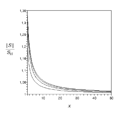
Figure 2: Evolution of the ratio between the absolute value of the phantom entropy and the horizon entropy for the model of Ref. sami . The graphs correspond successively to $\alpha$ values $1$, $2$, $3$, and $4$ from bottom to top. For convenience sake we have set $x_{i}=1$ in drawing the graphs. All the curves asymptote to $x$ = 1.

As an example of non-phantom dark energy with variable $w$ we consider the Chaplygin gas chaplygin . This fluid is characterized by the equation of state $P=-A/\rho$. Integration of the energy conservation equation yields $\rho=\sqrt{A+(B/a^{6})}$, whereby $w=-A\,a^{6}/(A\,a^{6}\,+B)$. Here $a$ is the scale factor normalized to its present value and $A$ and $B$ denote positive–definite constants. Accordingly, this fluid interpolates between cold matter, for large redshift, and a cosmological constant, for small redshift. This has led to propose it as a candidate to unify dark matter and dark energy unify .

The radius of the cosmological event horizon reads

$$R_{H}=\sqrt{\frac{\kappa}{3}}\,\frac{2}{A^{1/4}}\,x^{1/6}\,\left[1.4712-x^{1/12}\,\,_{2}F_{1}\left(\frac{1}{12},\frac{1}{4},\frac{13}{12};-x\right)\right]\,,$$ (16)

where ${}_{2}F_{1}$ is the hypergeometric function and $x=A\,a^{6}/B$ is a dimensionless variable. As figure 3 illustrates, $\mbox{Lim}_{\,x\rightarrow\infty}\,R_{H}=\sqrt{3/\kappa}\,A^{-1/4}$ which is nothing but the value taken by $H^{-1}$ in that limit. This was to be expected: for large scale factor the Chaplygin gas expansion goes over de Sitter’s.

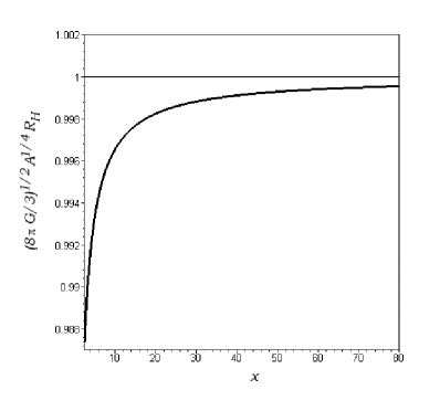
Figure 3: Evolution of the adimensionalized radius of the event horizon in the Chaplygin gas model. It tends to unity for $x\rightarrow\infty$.

The horizon temperature is

$$T_{H}=\frac{\hbar\,c}{2\pi\,k_{B}}\,\sqrt{\frac{\kappa}{3}}\,A^{1/4}\,\left(\frac{1+x}{x}\right)^{1/4},$$ (17)

while the entropy of the fluid and the entropy of the horizon evolve as

$$dS=-\frac{48k_{B}\,\pi^{2}}{\hbar\kappa^{2}\,A^{1/2}}\,\frac{1}{x^{2/3}(1+x)}\left[1.4712-x^{1/2}\,\,_{2}F_{1}\left(\frac{1}{12},\frac{1}{4},\frac{13}{12};-x\right)\right]^{2}\,dx\,,$$ (18)

and

$$dS_{H}=\frac{16k_{B}\,\pi^{2}}{\hbar\kappa^{2}\,A^{1/2}}\,x^{1/6}\,\left[1.4712-x^{1/2}\,\,_{2}F_{1}\left(\frac{1}{12},\frac{1}{4},\frac{13}{12};-x\right)\right]$$ (19)

$$\times\left\{2x^{-5/6}\left[1.4712-x^{1/2}\,\,_{2}F_{1}\left(\frac{1}{12},\frac{1}{4},\frac{13}{12};-x\right)\right]-\frac{1}{x^{3/4}\,(1+x)^{1/4}}\right\}\,,$$

respectively. The two latter equation imply that $\dot{S}\,+\,\dot{S}_{H}\geq 0$ for $x\geq 2.509$ or equivalently, for $\rho_{i}\leq 1.18A^{1/2}$. Thus, there is an early period in which the GSL seems to fail. However, this might be seen not as a failure of the GSL but as an upper bound on the initial value of the energy density of the Chaplygin gas.

Notice that, $S$ is a positive, ever–decreasing function of the scale factor that complies with the holographic bound $S\leq S_{H}$.

IV The issue of negative entropies

The fact that $S<0$ looks troublesome. In particular, it tells us that the entropy of the phantom fluid is not to be understood as a measure of the number of microstates associated to the macroscopic state of the fluid, i.e., the well-known statistical mechanics formula $S=k_{B}\,\ln W$ breaks down. However, the fact remains that the entropy of systems violating that condition ($w<-1$) is found to be negative (see also, pollock ; snegative ) whence one is rightly entitled to wonder whether these systems can be realized in nature. While the answer to this question lies beyond our present capabilities we may try to advance some ideas, pending a deeper study. First, we wish to recall that no physical law asserts that the entropy of a system has to be positive, the second law of thermodynamics simply establishes that the entropy of isolated systems cannot decrease. Secondly, one may draw a rough formal analogy between dark energy fluids with equation of state $P=w\rho$ and a very well known physical system, the mono-atomic ideal gas. The entropy of the latter is given by the Sackur–Tetrode equation (see Eq. (9.54) of Ref. huang ), which can be written as

$$\frac{\sigma}{k_{B}}=\frac{3}{2}-\ln\left[\left(\frac{2\pi\hbar^{2}}{mk_{B}\,T}\right)^{3/2}\,n\right]\,,$$

where $\sigma$ is the entropy per particle, $m$ the particle mass, and $n$ the particle number density. Clearly, by lowering the temperature below $T_{c}=(2\,\pi\hbar^{2}/e\,m)\,n^{2/3}$ the entropy becomes negative and the pressure, $P=2n\varepsilon/3$, with $\varepsilon$ the energy per particle, decreases accordingly (though it stays positive). Thus, by lowering $P$ (at fixed $n$) negative entropies can be formally attained. Obviously, one can argue that before a negative entropy state could be reached quantum effects would invalidate the approximations leading to the Sackur-Tetrode equation, and that, in any case, the gas would condensate ahead of that state.

This is somewhat analogous to a dark energy fluid whose pressure is steadily decreased by lowering $w$. When the $w=-1$ divide is crossed, the entropy becomes negative but simultaneously quantum instabilities might destroy the state carroll .

So, we are at a cross-road: either states violating the dominant energy condition are to be banned (as they entail negative entropies) or statistical mechanics is to be generalized to encompass these states. It is for the reader to decide which path to follow.

V Quasi-duality between phantom and non-phantom thermodynamics

The duality transformation

$$\left\{\begin{array}[]{ll}H&\rightarrow\overline{H}=-H\\ \rho+P&\rightarrow\overline{\rho}+\overline{P}=-(\rho+P)\end{array}\right.$$ (20)

leaves the Einstein’s equations

$$\begin{array}[]{ll}H^{2}=\frac{\kappa}{3}\rho,&\\ \dot{\rho}+3H(\rho+P)=0,&\\ \dot{H}=-\frac{1}{2}\kappa(\rho+P),&\end{array}$$ (21)

of spatial FRW universes invariant and the scale factor transforms as $a\rightarrow\overline{a}=1/a$ duality . Thus, a phantom dominated universe with scale factor $a=1/(-t)^{n}$ (for simplicity we assume a phantom scale factor as Eq. (1) with $t_{*}=0$ and $t<0$ that tends to $0^{-}$) becomes a contracting universe whose scale factor obeys $\overline{a}=(-t)^{n}$. This universe begins contracting from an infinite expansion at the infinite past and collapses to a vanishing scale factor for $t=0^{-}$ (left panel of Fig. 4).

Reversing the direction of time (i.e., the future of $t$, $t+dt$, transforms into $t-dt$), the contracting universe is mapped into an expanding one whose scale factor grows with no bound as $t$ tends to $-\infty$. Notice that the first transformation takes the universe from expanding to contracting and the second transformation makes the universe expand again, i.e., the final cosmology has $\widetilde{\overline{H}}>0$. It should be remarked that the latter transformation also preserves Eqs. (LABEL:einsteinequations).

Under these two successive operations, the final and the initial equation of states parameters are related by $w\rightarrow\widetilde{\overline{w}}=-(w+2)$. Consequently, phantom dominated universes with $n>1$, (i.e., $-5/3<w<-1$) are mapped into non-phantom dark energy dominated universes (see Fig. 4). Therefore, both of them, the original and the transformed universes, have an event horizon and entropies whose relation we derive below.

The radius of the event horizon of the original universe is $R_{H}=(-t)/(1+n)$ meanwhile the radius of the event horizon of the transformed universe is $\widetilde{\overline{R}}_{H}=(-t)/(n-1)=R_{H}[(1+n)/(1-n)]$. The transformations preserve the horizon temperature as the Hubble factor does not change. From the definition of the horizon, it is readily seen that

$$\frac{dR_{H}}{dt}=HR_{H}-1.$$ (22)

In virtue of the above expression together with the Gibbs equation one obtains

$$T\frac{dS}{dt}=-4\pi(\rho+P)R_{H}^{2},$$ (23)

whereby, the entropy transforms as

$$S\rightarrow\widetilde{\overline{S}}=-[(1+3w)/(5+3w)]^{2}S\,.$$ (24)

Therefore, the entropy of the final non-phantom dark energy dominated universe is proportional, but of the opposite the sign, to the entropy of the original phantom universe. We might say that the duality transformation “quasi” preserves the thermodynamics of dark energy. This result is in keeping with the findings of Section II.

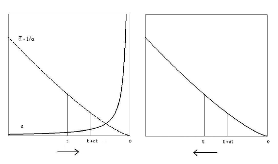
Figure 4: The left panel depicts the scale factor of the original phantom dominated universe (solid line). The dashed line shows the evolution of the scale factor dual of this phantom DE model, a contracting universe. In both models (the phantom and its dual) the time grows from left to right as tends to $t=0^{-}$ and the instant $t+dt$ lies at the future of the instant $t$. In the right panel, the time direction is reversed ($t+dt$ lies at the past of $t$). Under this operation, the contracting model of the left panel becomes the non-phantom DE dominated universe of the right panel if $-5/3<w<-1$.

VI Concluding remarks

We have substantially extended the study of Pollock and Singh pollock , who considered the models of super–inflation (characterized by $\dot{H}>0$) of Starobinsky starobinsky and Shafi and Wetterich shafi , by taking up models of accelerated expansion (both with $\dot{H}>0$ and with $\dot{H}<0$) with $w$ constant as well as models with $w$ variable (such as the model of Sami and Toporensky sami and the Chaplygin gas model chaplygin ).

We have found that, irrespective of whether $w$ is constant or not, phantom fluids (associated with $\dot{H}>0$) possess negative entropy, transcend the holographic bound in the sense that $\mid S\mid\geq S_{H}$ and their temperature and entropy increase as the Universe expands. By contrast, non-phantom fluids (associated with $\dot{H}<0$) have positive entropy, satisfy the holographic bound, $S\leq S_{H}$, and their temperature and entropy decrease with expansion. Except for the Chaplygin gas model which violates the GSL at the earliest stage of dominating the expansion, the GSL is fulfilled in all the cases.

It goes without saying that negative entropies are hard to assimilate, they have no clear physical meaning in the context of statistical mechanics; especially because the Einstein–Boltzmann interpretation of entropy as a measure of the probability breaks down. Systems of negative entropy appear to lie outside the province of statistical mechanics as is currently formulated populated ; huang ; mazenko . However, if future cosmic observations conclude that definitely $w<-1$, it will become mandatory to generalize that subject accordingly. We wish to emphasize that the laws of thermodynamics do not entail by themselves that $S$ ought to be a positive quantity. The latter will be found to be positive or negative only after combining these laws with the equation (or equations) of state of the system under consideration. What we believe to be at the core of thermodynamics is the law that forbids the entropy of isolated systems to decrease, this law encompasses the GSL for gravitating systems with a horizon. Another interesting result is that, unlike recent claims pedro , the temperature of the phantom fluid must be positive if the GSL is to be satisfied (see Eq. (6)). In our view, this settles the dispute between those rejecting phantom energy on grounds that it cannot be physically acceptable because its entropy is negative snegative and those who evade negative entropies by advocating negative temperatures instead pedro . Both approaches overlook the role of the event horizon.

As pointed out by Nojiri and Odintsov, it may well happen that in the last stages of phantom dominated universes the scalar curvature grows enough for quantum effects to play a non-negligible role before the big rip. If so, the latter may be evaded or at least softened nojiri . While our study does not incorporate such effects they should not essentially alter our conclusions so long as the cosmic horizon persists.

It is noteworthy that the duality transformation $\rho+P\rightarrow-(\rho+P)$ -see, e.g. duality - along with reversing the direction of time (i.e., $dt\rightarrow-dt$) leaves Einstein’s equations invariant and maps phantom cosmologies, with both $H$ and $\dot{H}$ positive, into non-phantom cosmologies with $H>0$ but $\dot{H}<0$ . However, this duality does not necessarily extend to the thermodynamics of the respective universes since future event horizons exist only when $\ddot{a}>0$. Nevertheless, in the particular case of pole-like expansions, Eq. (1), the transformation preserves the temperature while the entropy transforms according to Eq. (24) with the constraint $-5/3<w<-1$. More general instances will be considered elsewhere.