Constraining the properties of spots on
Pleiades very low mass stars

We present results of a multi-filter monitoring campaign for very low mass (VLM) stars in the Pleiades. Simultaneous to our I-band time series (Scholz & Eislöffel 2004b ), which delivered photometric periods for nine VLM stars, we obtained light curves in the J- and H-band. One VLM star with $M\approx 0.15\,M_{\odot}$ (BPL129) shows a period in all three wavelength bands. The amplitudes in I, J, and H are 0.035, 0.035, and 0.032 mag. These values are compared to simulations, in which we compute the photometric amplitude as a function of spot temperature and filling factor. The best agreement between observations and models is found for cool spots with a temperature contrast of 18-31% and a very low surface filling factor of 4-5%. We suggest that compared to more massive stars VLM objects may have either very few spots or a rather symmetric spot distribution. This difference might be explained with a change from a shell to a distributed dynamo in the VLM regime.

1 Introduction

Magnetic activity is an ubiquitous phenomenon on late-type stars. It shows up as coronal X-ray emission (e.g., Feigelson & Decampli fd81 (1981), Schrijver et al. smw84 (1984), Stauffer et al. scg94 (1994)) or as chromospheric emission in lines like H$\alpha$ and CaH&K (e.g., Wilson w78 (1978), Soderblom s85 (1985), Henry et al. hsd96 (1996)). In the photosphere, the most obvious indication for magnetic activity is the existence of dark star spots.

Probably the best way to investigate properties and evolution of these magnetic spots is to construct two-dimensional Doppler images from a spectroscopic time series. Such Doppler images are available for a number of late-type stars at various evolutionary stages, and they clearly show the existence of large, cool spots, which are in most cases asymmetrically distributed (e.g., Vogt et al. vph87 (1987), Piskunov et al. ptv90 (1990)). A more indirect way to investigate surface spots is photometric monitoring: Late-type stars often show a periodic light curve, and the best explanation for this behaviour is the flux modulation by cool spots co-rotating with the objects (e.g., Bouvier & Bertout bb89 (1989), Strassmeier s92 (1992)). It is possible to assess the spot properties, such as temperature and size, by monitoring large samples of targets in more than one filter as done by, e.g., Herbst et al. hhg94 (1994) and Bouvier et al. bck95 (1995) in the case of T Tauri stars.

In the last few years, it has become clear that phenomena which are usually attributed to magnetic activity do also occur on very low mass (VLM) stars, i.e. stars with masses below $0.4\,M_{\odot}$. At least down to spectral types of M7-M9, these objects show both X-ray (Mokler & Stelzer ms02 (2002)) and H$\alpha$ emission (e.g., Mohanty & Basri mb03 (2003)), indicating the presence of coronal and chromospheric activity. A significant fraction of VLM objects also shows periodic photometric variability, and it is commonly believed that these variations have their origin in magnetic surface spots (e.g., Herbst et al. hbm02 (2002), Scholz & Eislöffel 2004a , Lamm et al. lmb05 (2005)).

In the past, little information has been obtained about the properties of spots on VLM stars. This is mainly due to the fact that these objects are very faint, which makes it difficult to obtain high signal-to-noise spectra and light curves. Such studies are, however, very interesting, since for two reasons we expect a change of the spot characteristics in the VLM regime: a) Stars with $M<0.35\,M_{\odot}$ are believed to be fully convective (Chabrier & Baraffe cb97 (1997)). Therefore, they cannot form a solar-type $\alpha\Omega$-dynamo, which operates in a shell between convective and radiative zone (Parker p75 (1975), Spiegel & Weiss sw80 (1980)). Thus, there has to be a different mechanism for magnetic field generation, which may have consequences for the spots. b) VLM objects have very low effective temperatures compared to solar-mass stars. This reduces the coupling between magnetic field and gas. Thus, we should expect a decrease of magnetic activity as the objects become cooler.

Only recently, the advent of wide-field detectors made it possible to obtain large samples of periodic light curves of VLM objects, mainly for targets in very young clusters like the Trapezium cluster (Herbst et al. hbm01 (2001), hbm02 (2002)) and NGC2264 (Lamm l03 (2003), Lamm et al. lbm04 (2004), lmb05 (2005)). From our own monitoring campaigns, we published about 60 new periods for VLM objects in the clusters $σ$ Ori (Scholz & Eislöffel 2004a ), Pleiades (Scholz & Eislöffel 2004b , hereafter SE), and $ϵ$ Ori (Scholz & Eislöffel se05 (2005)). These studies give evidence for a change of the spot properties at very low masses: In the young cluster NGC2264, the amplitudes in the I-band lightcurves of the (non-accreting) VLM stars are on average reduced by a factor of 2.7 in comparison with more massive stars (Lamm l03 (2003)). VLM stars in the Pleiades show a similar behaviour. Their average amplitudes in their I-band lightcurves are reduced by a factor of four in comparison with V-band amplitudes of more massive stars. Such a comparison overestimates the difference in the amplitudes, since for any fixed combination of spot temperature and filling factor the amplitudes are always smaller in the I-band than in the V-band. However, even after converting the I-band amplitudes for VLM objects to the V-band using synthetic spectra, the VLM lightcurve amplitudes in the Pleiades are still at least a factor of 2.4 smaller than those of solar-mass objects (see Scholz s04 (2004)). Thus, for objects with masses below 0.3-$0.4\,M_{\odot}$, corresponding to spectral type M3-M4, the average light curve amplitudes tend to be smaller with respect to the higher mass objects (although there are still a few M dwarfs with relatively high amplitudes, e.g. GT Peg or YZ CMi, see Messina et al. mrg01 (2001)).

Since the distribution of the amplitudes depends only on the spot properties, the random orientation of the rotational axes, and the rotational properties, this decrease of the amplitudes requires different spot characteristics in comparison with solar-mass stars in the same rotational regime. At least four scenarios are possible: a) low spot coverage, b) low temperature contrast between spots and photospheric environment, c) a small degree of asymmetry in the spot distribution, d) most spots are polar spots.

Doppler images have been obtained for a few stars with spectral types around M2, (Barnes & Collier Cameron bc01 (2001)). These maps show many spots distributed mainly at low latitudes, which might exclude the scenarios a) and d) above. The stars for which Doppler images have been taken, however, have masses around or above $0.4\,M_{\odot}$. Thus, they are probably at the upper limit of the mass range where the photometric amplitudes decrease.

The first multi-filter monitoring study for VLM objects has been published by Terndrup et al. (tkp99 (1999)). For HHJ-409, a Pleiades star with $M=0.39\,M_{\odot}$, they measured amplitudes of 0.035 in the I- and 0.08 in the V-band. This is rather low in comparison with more massive Pleiades stars, though HHJ-409 has a rotation period of only 6 h, i.e. it is in a ’saturated’ rotational regime, where actually solar-mass stars tend to show decreased amplitudes (Messina et al. mrg01 (2001)). From these results, Terndrup et al. (tkp99 (1999)) derive a temperature contrast of 200 K (6%) and a surface filling factor of 13% for cool spots on HHJ-409, a Pleiades star with $M=0.39\,M_{\odot}$. For comparison, solar-mass stars show surface filling factors up to 25% and temperature contrast between 5 and 40% (e.g., Strassmeier s92 (1992)). The filling factor of the VLM star observed by Terndrup et al. thus is a rather typical value, but the temperature difference seems to be quite low. Hence, the result of Terndrup et al. (tkp99 (1999)) might indicate that a low temperature contrast is the reason for the decreased lightcurve amplitudes on VLM objects. However, this object still has a mass at the upper limit of the VLM regime, and it is therefore doubtful whether it is prototypical for this object class. Similar observations for objects with masses well below $0.3\,M_{\odot}$ are needed.

In this paper, we set out to explore the spot properties for VLM stars in the Pleiades by analysing their lightcurve amplitudes. Thus, we apply basically the same technique which has been successfully used for more massive stars in the past. This paper is structured as follows: Sect. 2 describes our photometric monitoring campaign in the near-infrared J- and H-bands, carried out in parallel with our published I-band time series in the Pleiades (SE). For these three wavelength bands, we determine photometric amplitudes in Sect. 3. These results are then compared to amplitudes derived from simulations (Sect. 4).

2 Near-infrared monitoring

Our I-band time series in the Pleiades was obtained with the CCD camera at the 1.23-m telescope on Calar Alto. It delivered high-precision light curves for 26 VLM stars in this cluster, from which we were able to determine nine photometric rotation periods (see SE). To complement these I-band data, we aimed for simultaneous monitoring in the near-infrared J- and H-bands to determine spot properties. In the following we describe these observations, as well as the derivation of the NIR light curves.

2.1 Observations and image reduction

In the last three nights of our I-band observations (from 17 to 19 October 2002), we observed the same target objects also with the 2.2-m telescope on Calar Alto, equipped with the near-infrared camera MAGIC (see Herbst et al. hbb93 (1993)). With MAGIC in wide-field mode, we obtained a field of view of $7^{\prime}\times 7^{\prime}$ and a pixel-scale of $1\aas@@fstack{\prime\prime}6$/pixel. The images in the I-band have a size of $17^{\prime}\times 17^{\prime}$, and we observed two fields in the I-band time series. At the time of the observations, we did not know which of the targets would be variable, thus we tried to cover most of them also in the NIR time series. This was possible with eight MAGIC pointings within the two I-band fields.

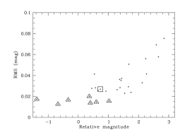
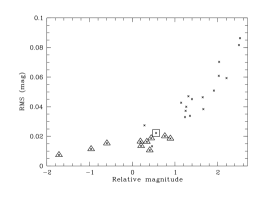
Figure 1: RMS for the J-band (upper panel) and H-band (lower panel) time series. Small crosses show the values for all sources in the object catalogue. Overplotted triangles mark the reference stars, which were used for the relative calibration. The overplotted square marks the object BPL129.

The observations were carried out with the following strategy: We started with a full J-band sequence over all eight fields, where the exposure time per field was $13\times 5$ s. Subsequently, the same sequence was repeated in the H-band, this time with exposure times of $19\times 5$ s. The first frame of each exposure was removed because it generally suffers from irregular bias variations. The remaining frames were summed up, so that we obtain one image per field, filter, and sequence. Thus, the exposure times for each data point were 60 sec in the J- and 90 sec in the H-band, which should give us similar signal-to-noise in both filters.

This whole sequence of 8 fields in J- and H-band, was executed throughout the nights, weather permitting. In the first night, observations had to be stopped after five and a half sequences because of cloud cover. A software problem restricted the observations in the second night to 13 sequences, and in the third night we obtained 14 full sequences. Altogether, we have 33 data points for each field in the J-band and 32 in the H-band. Apart from the first night, the atmospheric conditions were mostly photometric.

The data reduction of our NIR images uses standard techniques, but pays attention to the fact that we want to obtain as precise as possible photometry. We bias-corrected all our images and flat-fielded them with skyflats constructed by averaging the science frames and rejecting objects with a sigma clipping procedure. Sky-subtraction was performed using the xdimsum package in IRAF (Stanford et al. sed95 (1995)). This procedure determines the background for each science frame as running average of a number of $n$ images taken before and after the image of interest, after excluding the objects. We performed this procedure for each of our sequences of J- and H-band images individually. The number $n$ of images used in the determination of the sky-background is crucial for the final accuracy of our photometry. A larger number of frames leads to less noise in the sky background, since more images are averaged. On the other hand, the sky background may be variable on timescales on the order of the length of our sequence as a consequence of variable weather conditions. Hence, using too many images will introduce errors. To obtain the best choice for $n$ we varied this parameter from six to eight for each image. For our final photometry the background corrected image with the smallest background noise was used. For most images the best result was achieved with $n=8$, which confirms that the weather conditions were mostly stable at least over one full sequence, which enables reliable background subtraction for all images of the sequence.

2.2 Photometry and relative calibration

For all eight MAGIC fields, we created an object catalogue from a time series image with good seeing. Subsequently, we measured instrumental magnitudes by aperture photometry. The choice of the aperture radius has to account for the seeing during the observations, which varied between 1.0 and 1.8 pixels in the J-band. In the H-band, the average point spread function was about 0.2 pixels larger, due to a slight defocusing. Choosing a fixed aperture of 3 pixels, we include $>99$% of the stellar flux for all images.

The relative calibration of the instrumental light curves was carried out following the recipe presented in Scholz & Eislöffel (2004a ). In a first step, images with unreliable photometry were identified, i.e. images which deliver outlying data points for most objects, caused by strong background gradients or an excessive amount of cosmics. Note that these images have no influence on the sky subtraction (Sect. 2.1), because the running average procedure in xdimsum excludes ’bad images’ reliably. Since they might, however, disturb the photometry, we excluded them from further analysis. The basic principle of the relative calibration is to construct a mean light curve from a set of non-variable reference stars. These stars were selected by comparing the light curve of each reference star with the mean light curve of all other reference stars. With this procedure, we selected typically 5-10 stars which are non-variable with respect to all other stars. Their mean light curve was subtracted from the time series of our Pleiades targets. In Fig. 1, we illustrate the results of the relative calibration by plotting the RMS for all light curves in one MAGIC field. The values for the reference stars and a target star (in this case: BPL129) are marked. For the brightest objects, we typically reach a mean precision of 15-20 mmag both in the J- and the H-band.

3 Amplitude fitting

Phased light curves for all Pleiades targets in the I-, J-, and H-band were calculated from the period and zero point of the I-band time series analysis described in SE. Since period and zero point are fixed, only amplitudes remain to be determined. To improve the signal-to-noise ratio, we applied a moving median filter to the near-infrared phased light curves by averaging over three consecutive data points in phase space. This procedure is legitimate, because the lightcurve shape does not change significantly over the observing nights, as can be seen from the high signal-to-noise I-band time series.

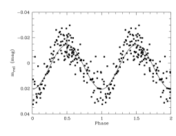
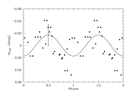
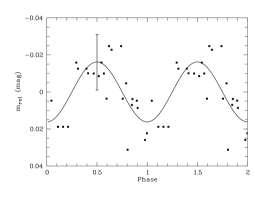
Figure 2: Phased light curves for BPL129 in the I-, J-, and H-band (from top to bottom). The solid lines shows the sine waves with the amplitudes for which the residuals are minimised. The error bar indicates the uncertainty for the derived amplitude.

As can be seen in the I-band light curves (SE), the light variations are usually well-approximated by a sine shape. Therefore, the amplitudes were determined by subtracting sine waves with the given period and zero point from the original light curve. We varied the amplitude until the residual noise was minimised. This procedure was carried out for amplitudes ranging from 0.001 to 0.1 mag, for all objects and filters.

For eight of our nine targets the signal-to-noise turned out too low to detect a significant amplitude in the NIR light curves. This is mainly due to the lower photometric precision in the NIR compared to the I-band, because of lower image quality and high background. The VLM star BPL129 (catalogue number of Pinfield et al. phj00 (2000)), however, shows a clearly defined period in the J- and H-band light curves (see Fig. 2). In all three filters, the residual noise has a clear minimum. We obtained amplitudes of 0.035 mag for the I-band, 0.035 mag for the J-band, and 0.032 mag for the H-band. Sine waves with these amplitudes are overplotted in Fig. 2.

Errors for these amplitudes can be determined from the noise of the residual light curve, i.e. after subtraction of the fitted sine wave. Using this method, we obtain 0.008 mag in the I-, 0.020 mag in the J-, and 0.011 mag in the H-band. This method works well with many data points, when the noise level is not significantly influenced by low number statistic. Thus, we adopt this error value for the I-band amplitude, where we have 160 data points. For the near-infrared light curves, with less data points, we decided to follow a different strategy for their error estimate: Averaging the rms of our non-variable reference stars (see Sect. 2.2), we are able to obtain a reliable estimate for the photometric precision. This gives us values of 0.017 mag in the J- and 0.015 mag in the H-band. Since these values are now based on the light curves of several stars, the statistical uncertainties are significantly decreased. We adopt these values as uncertainty of our amplitudes in the J- and H-band. We note that all these error estimates are conservative, since we do not make use of the fact that the sine fit uses all data points of the light curve. Instead, the error estimate is based on the photometric precision for one single data point.

4 Surface simulations

We now compare the observed lightcurve amplitudes with model calculations of the surface properties of VLM objects to constrain the temperature and the filling factor of spots on these objects. After a description of the method in Sect. 4.1, we use the I-band amplitudes for nine Pleiades VLM stars from SE for a first assessment of the spot properties in Sect. 4.2. In the subsequent Sect. 4.3, we focus on the object BPL129, for which we have derived near-infrared amplitudes in Sect. 3. Finally, we will compare our results with values for more massive stars (Sect. 4.4).

4.1 Description of the simulation

The amplitude of the light curve in this paper is defined as peak-to-peak magnitude difference. From our observations we have determined this value for three different wavelength bands. Thus the model should deliver the spectral energy distribution (SED) of the target in the maximum and the minimum of the light curve. In the following, we define as ’front side’ of the star the hemisphere which lies in the line of sight, whereas the ’backside’ is the hemisphere which is not visible for the observer at a given time.

The observed SED will be a mixture of the photospheric spectrum and the spectrum of the spots, which can either be cooler or hotter than the photosphere. This observed SED will change as a function of rotational phase. The prerequisite for our simulations is thus to know the SED dependence on effective temperature. For this study, we use the model spectra from the Lyon group, namely the models ’StarDUSTY2000’ which are NextGen models (Allard et al. aha97 (1997)), improved with new TiO opacities (Allard et al. ahs00 (2000)) and dust opacities (Allard et al. aha01 (2001)).

Table 1: Properties of our main target BPL129. Apparent magnitudes are from Pinfield et al. (phj00 (2000)) and from 2MASS, absolute magnitudes were derived adopting $E_{B-V}=0.03$ and a distance of 133 pc. The masses were obtained by comparing with the evolutionary track for 125 Myr of Baraffe et al. (bca98 (1998)).

Filter	m	M	Mass ($M_{\odot}$)
I	$16.25\pm 0.02$	$10.57\pm 0.06$	0.14
J	$14.27\pm 0.03$	$8.61\pm 0.06$	0.165
H	$13.72\pm 0.05$	$8.07\pm 0.08$	0.16
K	$13.40\pm 0.03$	$7.79\pm 0.06$	0.16

We estimate the effective temperature of our main target BPL129 with the available photometry: I-band data for BPL129 was published by Pinfield et al. (phj00 (2000)), and we obtained additional near-infrared data from 2MASS. These values are listed in the first row of Table 1. The J-, H-, and K-band photometry was shifted from the 2MASS system to the CIT system using the colour transformations given by Carpenter (c01 (2001)). The apparent magnitudes were de-reddened adopting a reddening of $E_{B-V}=0.03$ (Stauffer et al. ssk98 (1998)) and the extinction law of Savage & Mathis (sm79 (1979)). We adopt a distance of 133 pc to the Pleiades, a value which is consistent with all recent measurements except for the Hipparcos value (see Pan et al. psk04 (2004), Munari et al. mds04 (2004)). Thus, we obtain absolute magnitudes for BPL129 which are listed in Table 1.

The most probable age of the Pleiades is 125 Myr (Stauffer et al. ssk98 (1998)). To estimate the basic parameters of BPL129, we therefore compared the absolute magnitudes with the 125 Myr isochrone of Baraffe et al. (bca98 (1998)). We obtain an object mass between 0.14 and $0.165\,M_{\odot}$, depending on the wavelength band in which the comparison is carried out. Averaging over all four available photometry points, gives us $0.156\,M_{\odot}$ as mass estimate of BPL129, corresponding to an effective temperature of $3205\pm 100$ K. Therefore, we use the model spectrum with $T_{\mathrm{eff}}=3200$ K as SED for the photosphere of BPL129 (called $S_{0}$ in the following). Since the surface gravity for VLM stars in the Pleiades is best modelled with $\log{g}=5.0$ (Baraffe et al. bca98 (1998)), we used only the spectra for this gravity.

The spots will have either lower or higher effective temperatures. We decided to vary the effective temperature of the spots $T_{S}$ in the simulation between 2000 and 4000 K in steps of 100 K. With this grid of temperatures, the contrast between photosphere and spots $(T_{S}-T_{\mathrm{eff}})/T_{\mathrm{eff}}$ varies in the range from 0-38% for cool and 0-25% for hot spots, which are typical values for solar-mass stars (Strassmeier s92 (1992)). The SED of the spots is called $S_{S}$ in the following. Since we do not have information about the spot distribution, we assume here that there is one spot on the surface of the target, whose temperature and size are to be determined. For the surface filling factor of the spot, i.e. the fraction of the surface of a hemisphere covered by the spot, we choose values between 0.01 and 0.5 in steps of 0.01.

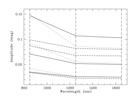
Figure 3: Photometric amplitudes in three wavelength bands as calculated in our simulations. Solid lines show the amplitudes for a constant spot temperature of $T_{S}=2700$ K with filling factors 0.05, 0.1, 0.2 (from bottom to top). Dashed lines show the results for constant filling factor of 0.1, but for $T_{S}=2300$, 2500, and 3000 K (from top to bottom). Dotted lines are for hot spots with constant filling factor of 0.1 and $T_{S}=3400$, 3600, 3800 K (from bottom to top).

First we assume that the spot is cooler than the photosphere. Then in the light curve minimum, the spot will be on the front side, in the maximum on the backside. Under these conditions, the SED in the maximum $S_{\mathrm{max}}$ is just $S_{0}$ and in the minimum:

$$S_{\mathrm{min}}=(1.0-f)\times S_{0}+f\times S_{S}(T_{S})$$ (1)

where $f$ is the filling factor of the spots and $T_{S}$ is between 2000 and 3200 K. These SEDs for maximum and minimum are now convolved with transmission curves for the I-band and the CCD sensitivity curve, or with transmission curves for J- or H-band. By integrating over the respective SEDs, we compute the flux in the minimum and maximum in all three filters, called $F_{\mathrm{min,I}}$, $F_{\mathrm{min,J}}$, $F_{\mathrm{min,H}}$ and $F_{\mathrm{max,I}}$, $F_{\mathrm{max,J}}$, $F_{\mathrm{max,H}}$. The amplitude for the wavelength band X can then be calculated with:

$$A_{X}=-2.5\log{\frac{F_{\mathrm{min,X}}}{F_{\mathrm{max,X}}}}$$ (2)

These amplitudes were calculated for the grid of the parameters $f$ and $T_{S}$ given above. A very similar calculation was carried out for hot spots. In this case, the SED in the minimum is $S_{0}$, and the SED in the maximum is given by Equ. (1), now for $T_{S}>3200$ K. As the result of the simulations, we obtain a table giving $A_{I}$, $A_{J}$, and $A_{H}$ for the complete grid of spot temperatures and filling factors.

In Fig. 3, we show the amplitudes as a function of wavelength for a few selected combinations of $T_{S}$ and $f$. Solid lines give the amplitudes for a constant spot temperature of $T_{S}=2700$ K with filling factor 0.05, 0.1, 0.2. Dashed lines show the results for constant filling factor of 0.1, but for $T_{S}=2300$, 2500, 3000 K. Dotted lines are for hot spots with constant filling factor of 0.1 and $T_{S}=3400$, 3600, 3800 K. The plot clearly demonstrates that different spot parameters lead to significantly different photometric amplitudes. If either the spot temperature or the filling factor is fixed, the amplitudes vary continuously with the second parameter. On the other hand, the problem is degenerate in the sense that many combinations of $T_{S}$ and $f$ lead to very similar amplitudes, which cannot be distinguished by observations. Thus, we do not expect to be able to derive the exact values for $T_{S}$ and $f$ by comparing with observations, but rather to constrain the parameter space. Hot spots show a much steeper decrease of the amplitude towards red wavelengths, which can be used to distinguish them from cool spots.

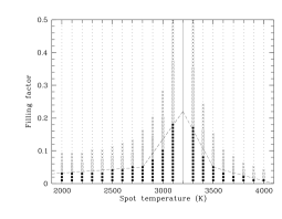
Figure 4: Constraints for the spot parameters from the observed I-band amplitudes: Filled squares show all possible combinations of filling factor and spot temperature which would produce an I-band amplitude of $<0.035$ mag, the upper limit of the observed amplitudes. The dashed lines are a rough envelope of these values. Empty squares are spot parameters for amplitudes between 0.035 and 0.07 mag, crosses for amplitudes between 0.07 and 0.1 mag, small dots for values $>0.1$ mag. The solid line shows the photospheric temperature of our main target BPL129.

There are three limitations of our method: First, we can only investigate the part of the spots, which is asymmetrically distributed, because the symmetric fraction of the spot distribution does not contribute to the photometric variability. Thus, the derived values for $T_{S}$ and $f$ give us only information about the ’asymmetric’ spots. This should not significantly bias the result for $T_{S}$, because there is no reason to assume that the temperature of the spots on a particular object depends on their distribution. On the other hand, the values for the filling factor $f$ are only a lower limit, since there could be much more spot coverage without any asymmetry.

The second problem is the unknown orientation of the rotational axis of the object. In the simulation, we assume that the axis is perpendicular to the line of sight. An inclination of the rotation axis would decrease the influence of the spots on the light curve, in the sense that the amplitude would decrease by a wavelength independent constant. Thus, the amplitudes which we derive in the simulation, are upper limits for the given spot parameters. The assumption of an angle $i\approx 90$° between rotational axis and line of sight is, however, not unplausible for BPL129, which has the maximum I-band amplitude among our targets. Since the scatter of the amplitudes is partly caused by the scattering of $i$, we expect that objects with relatively high amplitudes (like BPL129) tend to have high inclination angles.

Furthermore, it has been shown e.g. by Messina et al. (mrg01 (2001)) that light curve amplitudes are related to the object rotation periods. Such a correlation – if it also applies to our targets – may introduce an additional scatter in the photometric amplitudes. A future determination of the inclination angles of the rotation axes of our targets should help to disentangle and quantify these effects, and requires additional observations.

4.2 Comparison with I-band amplitudes

I-band amplitudes have been measured for nine VLM stars in the Pleiades (SE). All these values are below 0.035 mag, which is the amplitude of BPL129, the star for which we derived amplitudes in the NIR. In addition, Terndrup et al. (tkp99 (1999)) present light curves for two VLM stars in this cluster: Whereas HHJ-409 has an amplitude of about 0.035 mag, consistent with the upper limit in SE, the second star, CFHT-PL-8, has a higher amplitude of about 0.07 mag. Since it is the only VLM object in the Pleiades with amplitude $>0.035$ mag, whereas all other ten objects with photometric periods show lower amplitudes, we treat this amplitude of 0.07 mag as an outlier, although this object clearly requires a more detailed investigation. Thus the upper limit for the photometric amplitudes in the I-band is assumed to be 0.035 mag.

This can be used to constrain the parameter space for the spot properties. In Fig. 4 we show spot temperature vs. filling factor for amplitudes $<0.035$ mag (filled squares), between 0.035 and 0.07 mag (empty squares), between 0.07 and 0.1 mag (crosses), and for amplitudes $>0.1$ mag (small dots). The solid line marks the photospheric temperature of BPL129. Our simulations were tailored for this object, in the sense that they are based on its effective temperature, but we do not expect qualitatively different results for the other objects: All known variable VLM objects in the Pleiades have effective temperatures between 3400 and 2900 K. Increasing or decreasing the values for $T_{\mathrm{eff}}$ by not more than 300 K would only shift the whole plot to higher or lower temperatures.

A dashed line marks the upper envelope of the filled squares and is an envelope for the range of spot parameters which could produce the amplitudes observed on VLM objects. Thus, the parameter space can be significantly constrained only with the I-band amplitudes: To explain the observed amplitudes, the filling factor has to be below 5% (with a temperature difference between 3 and 38%) or the temperature difference has to be below 10% (with a filling factor between 1 and 19%). If we include the 0.07 mag amplitude of CFHT-PL-8 (see above), even the solutions shown in open squares have to be considered, enlarging the spectrum of possible solutions. In this case, the filling factor has to be below 10% (with a temperature difference between 3 and 38%) and/or the temperature contrast has to be below 22% (with filling factors between 1 and 37%).

4.3 Constraints from NIR time series

Now we compare the results of our multi-filter results of BPL129 with the simulations. The amplitudes in I, J, and H are 0.035, 0.035, and 0.032 mag. A first evaluation of these values is possible with Fig. 3. Since the photometric amplitudes are below 0.04 mag, they can only be explained with low contrast between spots and photosphere, but filling factors up to 10%, or larger temperature contrast and filling factors below 5%, as already shown in Sect. 4.2. On the other hand, the amplitude does not show a sharp decrease from the I- to the J-band, indicating that the spots are probably cooler than the photosphere.

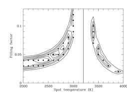
Figure 5: Contour plot for the $\chi^{2}$ values from the comparison between observed and simulated amplitudes. Contour lines start at $\chi^{2}=$3.0 and are plotted for $\chi^{2}=$3.0, 2.0, 1.5, 1.0, 0.75, 0.5, indicating increasing quality of the fit. Filled squares show all combinations of spot temperature and filling factor which would produce amplitudes within the error bars of our observations. The vertical solid line indicates the photospheric temperature of BPL129. Note that the hot spot solutions on the right side never reach to the 4th contour line, and $\chi^{2}$ is larger than 0.9 everywhere. They are thus significantly worse than the cool spot solutions on the left side. (One datapoint with $\chi^{2}=0.92$ at $T_{S}=3300$ K and $f=19$% is not shown in the figure.)

In Fig. 5 we show with filled squares all combinations of spot temperature and filling factor from our simulations, which are within the error bars of the measured amplitudes. Since our error estimates are very conservative, we can safely exclude that the spot parameters of BPL129 are not represented by this set of parameters. In agreement with the result from Sect. 4.2 we find that either the filling factor has to be between 2 and 5% or the temperature difference between spots and photosphere has to be lower than 10% to explain the observed amplitudes.

To assess the statistical significance of these results, we calculated $\chi^{2}$ for all data points: (obs - observed amplitudes, sim - simulated amplitudes)

$$\chi^{2}=\sum_{X=I,J,H}\Bigl{|}\frac{A_{\mathrm{X,obs}}-A_{\mathrm{X,sim}}}{\sigma_{\mathrm{X}}}\Bigr{|}^{2}$$ (3)

In Fig. 5 we show a contour plot of the results, with contours for $\chi^{2}=$ 3.0, 2.0, 1.5, 1.0, 0.75, 0.5, indicating increasing quality of the fit. The five solutions which deliver the minimum $\chi^{2}$ ($<0.5$) and thus the best agreement between simulated and observed amplitudes have filling factors of 4-5% and a spot temperature between 2200 and 2600 K, corresponding to a temperature contrast of 18-31%. The most probable spot configuration has $T_{S}=2400$ K and $f=4$%. Note that hot spot solutions show only up to three contour lines and give $\chi^{2}$ values $>0.9$. They are thus clearly less signficant than the best solutions with cool spots.

Recapitulating, we find that the best agreement between simulated and observed amplitudes is reached with very low filling factors of 4-5%. We like to stress once more that this is not the total surface filling factor. This value is only related to the asymmetrically distributed fraction of the spots. A low value for the filling factor means that either the total spot coverage is low or the spot distribution is rather symmetric. The best solutions are found for cool spots, where the temperature contrast between spots and photosphere is probably 18-31%.

4.4 Comparison with literature data

Our results are now compared to literature data for more massive stars. Spot parameters have been determined for a large number of solar-mass stars, at various evolutionary stages (see Bouvier & Bertout bb89 (1989), Strassmeier s92 (1992)). Both pre-main sequence and main sequence stars show a very large range of filling factors and spot temperatures. The temperature contrast varies between 5 and 40%, where the majority of the values is between 20 and 30%. Thus, the result of 18-31% which we obtain for BPL129 is not untypical when compared to solar-mass stars. On the other hand, according to Strassmeier s92 (1992), solar-mass stars show filling factors between 0 and 25% of the entire stellar surface. In our simulations, the filling factor is defined as the fraction of the stellar hemisphere covered with spots (see Sect. 4.1). Hence, the value derived for BPL129 (4-5%) would correspond to 2-3% if related to the entire stellar surface, and is thus at the low end of the range found for solar-mass stars. We come to the conclusion that BPL129 shows rather low filling factors compared to more massive stars.

As discussed in Sect. 1, there are at least two possible explanations for these results. The low filling factor measured for BPL129 might be caused by a change of the interior dynamo. It has often been discussed that the solar-type $\alpha\Omega$ dynamo, which operates in a shell between convective and radiative zone, might be replaced by a distributed dynamo in fully convective objects. This dynamo could be either of turbulent nature (Durney et al. ddr93 (1993)) or based on Coriolis forces, the so-called $\alpha^{2}$ dynamo (Kueker & Ruediger kr99 (1999)). A distributed dynamo should lead to a more symmetric spot distribution, which would decrease the filling factor of the asymmetric component of the spots (see Sect. 4.3).

Decreasing effective temperatures could also cause a low filling factor, because the cooler the objects, the less efficient is the coupling between magnetic field and gas. Indeed, a decline of the chromospheric and coronal activity is observed at late M spectral types (Mohanty & Basri mb03 (2003), Mokler & Stelzer ms02 (2002)). If the same decline does also occur in the photospheric regime, we should expect very few spots on objects with spectral type later than M9. It is, however, unlikely that the difference in effective temperature is the reason for the low filling factor measured for BPL129, since BPL129 is of mid-M spectral type, a region where VLM objects still show high levels of chromospheric and coronal activity. Thus, the low filling factor of BPL129 is more probably the consequence of a change of the interior dynamo than of the low effective temperature.

As already mentioned in Sect. 1, Terndrup et al. (tkp99 (1999)) estimated spot parameters for HHJ-409, a Pleiades VLM star with $M=0.39\,M_{\odot}$. They find a filling factor of 13% and a temperature contrast of 6%. These spot properties are clearly different from the best solutions we have found for BPL129 (see Sect. 4.3), and are in addition not contained among the solutions which are in agreement with the errorbars of our photometry (filled squares in Fig. 5). Thus, based on the multi-filter photometry HHJ-409 has spot parameters different from those of BPL129.

One explanation may be that Terndrup et al. (tkp99 (1999)) used a simple blackbody distribution to model the spectrum of photosphere and spots, which might be an unrealistic approach, given that the SEDs of very cool objects deviate strongly from a blackbody. On the other hand, the mass difference between BPL129 and HHJ-409 is significant. In particular, the mass of HHJ-409 is probably slightly above the limit where the objects become fully convective (see Sect. 1) leading to a different type of dynamo mechanism in operation. As explained above, this might be the reason for the different spot characteristics.

5 Conclusions

We investigate the spot properties of VLM objects by comparing the amplitudes of photometric variations in three wavelength bands with simulations. This study is based on the variability study in the Pleiades, which delivered I-band amplitudes for nine VLM stars (SE). All these amplitudes are $\leq 0.035$ mag. These VLM stars have been additionally monitored in the J- and H-band. For the star BPL129, which has an I-band amplitude of 0.035 mag, we were able to derive amplitudes of 0.035 and 0.032 mag in the J- and H-band.

The simulations are based on model spectra from Allard et al. (ahs00 (2000)), which give us the SED for the photosphere and for various spot temperatures. We compute the amplitude between the light curve minimum and maximum depending on the spot temperature and the filling factor by assuming that the star has one spot co-rotating with the object and the rotational axis is perpendicular to the line of sight. The filling factor in these simulations is determined by the fraction of the stellar hemisphere which is covered asymmetrically with spots.

In a first step, we compare only the I-band amplitudes with these models. We find that the filling factor has to be below 5% and/or the temperature contrast has to be below 10% to produce the observed I-band amplitudes. The data points in the J- and H-band for BPL129 can be used to further constrain the spot properties. We find best agreement between observed and simulated amplitudes with cool spots with temperatures 18-31% below the photospheric temperature and a filling factor of 4-5%.

These results are compared to similar studies for more massive stars. It turned out that spots on VLM stars have similar temperature contrast, but rather low filling factors when compared to solar-mass stars. This might be the consequence of a change of the dynamo from a solar-type shell dynamo to a distributed dynamo in these fully convective objects.

- (1) Allard, F., Hauschildt, P. H., Alexander, D. R., Starrfield, S., 1997, ARA&A, 35, 137
- (2) Allard, F., Hauschildt, P. H., Schwenke, D., 2000, ApJ, 540, 1005
- (3) Allard, F., Hauschildt, P. H., Alexander, D. R., Tamanai, A., Schweitzer, A., 2001, ApJ, 556, 357
- (4) Baraffe, I., Chabrier, G., Allard, F., Hauschildt, P. H., 1998, A&A, 337, 403
- (5) Barnes, J. R., Collier Cameron, A., 2001, MNRAS, 326, 950
- (6) Bouvier, J., Bertout, C., 1989, A&A, 211, 99
- (7) Bouvier, J., Covino, E., Kovo, O., Martin, E. L., Matthews, J. M., Terranegra, L., Beck, S. C., 1995, A&A, 299, 89
- (8) Carpenter, J. M., 2001, AJ, 121, 2851
- (9) Chabrier, G., Baraffe, I., 1997, A&A, 327, 1039
- (10) Durney, B. S., De Young, D. S., Roxburgh, I. W., 1993, SoPh, 145, 207
- (11) Feigelson, E. D., Decampli, W. M., 1981, ApJ, 243, 89
- (12) Henry, T. J., Soderblom, D. R., Donahue, R. A., Baliunas, S. L., 1996, AJ, 111, 439
- (13) Herbst, T.M., Beckwith, S.V., Birk, C., Hippler, S., McCaughrean, M.J., Mannucci, F. & Wolf, J. 1993, SPIE, 1946, 605
- (14) Herbst, W., Herbst, D. K., Grossman, E. J., Weinstein, D., 1994, AJ, 108, 1906
- (15) Herbst, W., Bailer-Jones, C. A. L., Mundt, R., ApJ, 554, 197
- (16) Herbst, W., Bailer-Jones, C. A. L., Mundt, R., Meisenheimer, K., Wackermann, R., 2002, A&A, 396, 513
- (17) Küker, M., Rüdiger, G., 1999, A&A, 346, 922
- (18) Lamm, M. H., 2003, Ph.D. thesis, University of Heidelberg
- (19) Lamm, M. H., Bailer-Jones, C. A. L., Mundt, R., Herbst, W., Scholz, A., 2004, A&A, 417, 557
- (20) Lamm, M. H., Mundt, R., Bailer-Jones, C. A. L., Herbst, W., 2005, A&A, 430, 1005
- (21) Messina, S., Rodono, M., Guinan, E. F., 2001, A&A, 366, 215
- (22) Mohanty, S., Basri, G., 2003, ApJ, 583, 451
- (23) Mokler, F., Stelzer, B., 2002, A&A, 391, 1025
- (24) Munari, U., Dallaporta, S., Siviero, A., Soubiran, C., Fiorucci, M., Girard, P., 2004, A&A, 418, 31
- (25) Pan, X., Shao, M., Kulkarni, S. R., 2004, Nature, 427, 326
- (26) Parker, E. N., 1975, ApJ, 198, 205
- (27) Pinfield, D. J., Hodgkin, S. T., Jameson, R. F., Cossburn, M. R., Hambly, N. C., Devereux, N., 2000, MNRAS, 313, 347
- (28) Piskunov, N. E., Tuominen, I., Vilhu, O., 1990, A&A, 230, 363
- (29) Savage B.H., Mathis J.S., 1979, ARA&A, 17, 73
- (30) Scholz, 2004, Ph.D. thesis, University of Jena
- (31) Scholz, A., Eislöffel, J., 2004, A&A, 419, 249
- (32) Scholz, A., Eislöffel, J., 2004, A&A, 421, 259 (SE)
- (33) Scholz, A., Eislöffel, J., 2005, A&A, 429, 1007
- (34) Schrijver, C. J., Mewe, R., Walter, F. M., 1984, A&A, 138, 258
- (35) Soderblom, D. R., 1985, AJ, 90, 2103
- (36) Spiegel, E. A., Weiss, N. O., 1980, Nature, 287, 616
- (37) Stanford, S.A., Eisenhardt, P.R.M, Dickinson, M. 1995, ApJ, 450, 512
- (38) Stauffer, J. R., Caillault, J.-P., Gagne, M., Prosser, C. F., Hartmann, L. W., 1994, ApJS, 91, 625
- (39) Stauffer, J. R., Schultz, G., Kirkpatrick, J. D., 1998, ApJ, 499, 199
- (40) Stelzer, B., Neuhäuser, R., Hambaryan, V., 2000, A&A, 356, 949
- (41) Strassmeier, K. G., 1992, ASP Conf. Ser., 34, 39
- (42) Terndrup D. M., Krishnamurthi A., Pinsonneault M. H., Stauffer J. R., 1999, AJ, 118, 1814
- (43) Vogt, S. S., Penrod, G. D., Hatzes, A. P., 1987, ApJ, 321, 496
- (44) Wilson, O. C., 1978, ApJ, 226, 379