Dependence of the non-linear mass power spectrum on the equation of state of dark energy

Abstract

We present N-body simulation calculations of the dependence of the power spectrum of non-linear cosmological mass density fluctuations on the equation of state of the dark energy, $w=p/\rho$. At fixed linear theory power, increasing $w$ leads to an increase in non-linear power, with the effect increasing with $k$. By $k=10~{}\,h\,{\rm Mpc}^{-1}$, a model with $w=-0.75$ has $\sim 12$% more power than a standard cosmological constant model ($w=-1$), while a model with $w=-0.5$ has $\sim 33$% extra power (at $z=0$). The size of the effect increases with increasing dark energy fraction, and to a lesser extent increasing power spectrum normalization, but is insensitive to the power spectrum shape (the numbers above are for $\Omega_{m}=0.281$ and $\sigma_{8}=0.897$). A code quantifying the non-linear effect of varying $w$, as a function of $k$, $z$, and other cosmological parameters, which should be accurate to a few percent for $k\tilde{<}10~{}\,h\,{\rm Mpc}^{-1}$ for models that fit the current observations, is available at http://www.cita.utoronto.ca/$\sim$pmcdonal/code.html. This paper also serves as an example of a detailed exploration of the numerical convergence properties of ratios of power spectra for different models, which can be useful because some kinds of numerical error cancel in a ratio. When precision calculations based on numerical simulations are needed for many different models, efficiency may be gained by breaking the problem into a calculation of the absolute prediction at a central point, and calculations of the relative change in the prediction with model parameters.

1 Introduction

Dark energy is the most important focus of study in cosmology today. Its basic existence is well established, both by observations of Type Ia supernovae (Knop et al., 2003; Riess et al., 2004), and by combinations of other observables (Seljak et al., 2005). The focus now is on probing the properties of the dark energy (or whatever new physics causes the Universe to look like it contains dark energy). A simple first parameterization of its properties is to specify the ratio of pressure to density (equation of state) $w=p/\rho$, with $w=-1$ for a cosmological constant.

The large amount of observational effort focused on measuring $w$ to high precision must be matched by sufficiently accurate predictions of the dependence of observables on $w$. Theory calculations will need to be done more carefully than they have been in the past. In particular, probes of $w$ based on cosmological structure (e.g., weak lensing, galaxy clusters, and even large-scale galaxy clustering where the linear power assumption is no longer exclusively relied on (Tegmark et al., 2004; Abazajian et al., 2004; Eisenstein et al., 2005)) will generally require non-linear numerical simulations as the fundamental method of calculating theory predictions. This paper tackles a small part of the problem: computing the dependence of the non-linear mass power spectrum, $P_{\rm NL}(k,z)$, on $w$.

The most direct use of calculations of the non-linear power spectrum is for weak gravitational lensing (cosmic shear) studies (e.g., Benabed & Van Waerbeke (2003); Simpson & Bridle (2004); Huterer & Takada (2005); Jarvis et al. (2005); Knox et al. (2005)). Direct use of the mass power for weak lensing (as opposed to ray tracing) is of course only as good as the Born and Limber approximations. Vale & White (2003) found the Born approximation agreed well with ray tracing, although this is less clear in White & Vale (2004). In a pilot project, White & Vale (2004) performed a small grid of simulations of weak lensing with full ray tracing, including $w=-0.8$, for parameter combinations designed to leave the CMB fluctuations invariant. When performing a full grid of models for precision parameter fitting, this CMB-guided method is probably the best way to go. Here we concentrate on isolating the effect of $w$ by running simulations where only $w$ and possibly one other parameter is varied at a time (although the fitting formula we present does include joint variations of $w$, $\sigma_{8}$, and $\Omega_{m}$). Even if ray tracing is ultimately required for high precision, it should still be useful to have an accurate mass power spectrum calculation, so we leave ray tracing for future work.

The fitting formulas most commonly used to predict the non-linear power spectrum given a set of cosmological parameters were not calibrated with $w\neq-1$ simulations (Peacock & Dodds, 1996; Smith et al., 2003), although Benabed & Bernardeau (2001) present an untested prescription for using Peacock & Dodds (1996). Often these formulas are used for $w\neq-1$ by making the untested assumption that models with equal linear theory power and other parameters (most importantly $\Omega_{m}$) at the redshift of interest will have equal non-linear power, independent of $w$. Ma et al. (1999) did simulate the mass power spectrum for $w=-2/3$, $-1/2$, and $-1/3$, and combined these with the $\Lambda$CDM simulations in Ma (1998) to produce a fitting formula. There is no obvious reason not to trust this formula to the 10% level of accuracy advertised; however, the grid of simulations used to calibrate it was sparse (e.g., the $w>-1$ simulations all had $\Omega_{m}\geq 0.4$), and numerical convergence was not rigorously demonstrated. We will find that this formula does not work well in the region of parameter space where we find ourselves. Klypin et al. (2003) simulated models with different values of $w$, but did not present the power spectrum in detail. The one case they did show, a Ratra & Peebles (1988) model with time varying $w\sim-0.5$, appears to be roughly consistent with our results.

We do not aim in this paper to replace the existing fitting formulas for the non-linear power – only to provide an accurate correction for $w\neq-1$. We generally consider flat models with parameters $\sigma_{8}$ (the rms linear mass density fluctuations in $8\,h^{-1}\,{\rm Mpc}$ radius spheres at $z=0$), $\Omega_{m}$, $\Omega_{b}$ (the mass and baryon densities relative to the critical density), $h$ (the Hubble parameter), $n$ (the logarithmic slope of the primordial power spectrum), and $w$. The dark energy equation of state parameter $w$ does not affect the shape of the transfer function on non-linear scales (e.g., $<0.5$% difference at $k>0.007~{}\,h\,{\rm Mpc}^{-1}$ between the transfer function for $w=-1$ and $w=-1/2$, from CMBFAST (Seljak & Zaldarriaga, 1996), for a typical model normalized at high-$k$), so the $z=0$ linear theory power is not changed at all by changing $w$, when our other parameters are fixed. There can be, however, a change in the non-linear power with $w$, because the growth history changes – increasing $w$ means the Universe had relatively more linear theory power at earlier times. This effect is not included in an estimate of the non-linear power made using something like the Smith et al. (2003) fitting function.

We will frequently refer to the change in observables with $w$ at fixed $z=0$ values of other parameters as “the effect of $w$.” We are not implying that there is anything uniquely correct about this. From some points of view it would make more sense to fix the other parameters at early times, before the dark energy has become significant. We focus on the former definition of the effect of $w$ simply because it is generally not included in weak lensing calculations (Huterer & Takada, 2005; Simpson & Bridle, 2004; Jarvis et al., 2005; Knox et al., 2005), and can not be reproduced in any obvious way using the existing codes. While it is mostly a matter of arbitrary definition, there is a real sense in which our choice is “the” non-linear effect of $w$ at $z=0$: our effect goes to zero in the limit of small perturbations.

The range of $k$ and $z$ we consider, and the accuracy goal, are guided by the weak lensing application ($k\equiv 2\pi/\lambda$, where $\lambda$ is the wavelength of a Fourier mode). We limit ourselves to the range $0<z<1.5$, because this range is most directly sensitive to the presence of dark energy and most relevant to galaxy weak lensing surveys, and because the power at increasing redshift should probably be simulated using decreasing box size, since limited particle density becomes an increasingly serious problem (the true small-scale power is smaller relative to the spurious particle discreteness-related power) while limited box size becomes less problematic (smaller scale modes are still linear). Huterer & Takada (2005) investigated the requirements on the $P_{\rm NL}(k,z)$ calculation for future large weak lensing surveys, finding that 1-2% accuracy should be sufficient, or 0.5% in the worst possible case. They found that the relevant scales are $0.1\tilde{<}k\tilde{<}10\,h\,{\rm Mpc}^{-1}$. Zhan & Knox (2004) studied the effect of hot baryons on the weak-lensing shear power spectrum in halo models. They found an effect of roughly 5-10% on the power at $k=10~{}\,h\,{\rm Mpc}^{-1}$ (reading from their Figure 1), so trying to achieve better than a few percent precision at this $k$ using simulations without gas dynamics is probably pointless (it is always good to aim for errors somewhat smaller than the other known sources). Zhan (2004) found roughly similar results in SPH simulations (reading from Figure 5.7), and White (2004) found a comparable scale for the effect of baryonic cooling. We will not actually achieve 1-2% level accuracy in the dependence of power on $w$, but we think we show a clear path to it. The accuracy we do achieve is substantially better than anything else available, so it should be useful until a larger project can improve it.

Throughout the paper, we use the trick of canceling numerical errors by taking ratios of power spectra for different models, rather than looking at the absolute power in each model directly. This should in no way be considered a swindle or an added approximation. It is completely reasonable and expected that many types of error are insensitive to the model, so that ratios (or differences) between the models can genuinely be computed more accurately than either model individually. One example of this is the effective smoothing involved in mapping particles to a grid so that you can FFT the periodic density field for the purpose of measuring the power. This suppresses the power substantially, but by precisely the same factor in all models. This factor cancels exactly when we take a ratio, up to some high $k$ where the power may be corrupted by aliasing, or the suppression is simply too large to invert accurately. The key to believing these results is that the convergence of the ratios of power with numerical parameters of the simulations must be tested carefully in the same way a direct measurement of the power would be. For example, taking ratios would not cancel an additive Poisson noise term due to the limited number of particles, but this would become completely obvious in a convergence test where the number of particles is varied.

We use a particle-multi-mesh (PMM) code, based on an improved particle-mesh (PM) algorithm, for our grid of N-body simulations. In principle, PM codes can achieve high spatial resolution but at a great cost in memory and to a lesser extent in work. In practice, they are normally limited to a mean interparticle spacing-to-mesh cell spacing ratio of 2:1, where the storage requirements for particles and grids are approximately balanced. PMM utilizes a domain-decomposed, FFT-based gravity solver (Trac & Pen, 2004; Merz et al., 2005) to achieve higher spatial resolution while maintaining memory costs. We will find that a ratio of 4:1 between the particle grid spacing and mesh grid spacing is roughly optimal, in the sense that at a given $k$ (the most relevant $k$ where the errors are a few percent) the error from limited particle density and limited force resolution are similar, for ratios of power spectra from simulations with different $w$. We note that Heitmann et al. (2004) compared several N-body codes (not including ours), looking at absolute power, and found good general agreement.

It can be useful to consider numerical errors rather carefully, focusing on the initial small breakdown of accuracy, because, for example, a factor of two change in resolved scale or required box size can easily change the require computer time or memory by a factor of at least eight. At least five things must be investigated in every simulation program: Sensitivity to starting redshift, box size, mass resolution (i.e., number of particles), force resolution, and time step size. We also test our method of power spectrum calculation. Even though not everything we find will be completely generalizable to other types of simulations, we think it is useful to lay out an attempt to push them all to a percent level of control.

Throughout this paper we use the philosophy of suppressing our urge to be general (e.g., increase the redshift range and parameter space coverage and study weak lensing directly) in favor of patiently investigating a restricted problem. I.e., rather than trying to entirely solve the problem of calculating the power spectrum over all parameter space, which at this point would require approximations and cutting corners, we select a small subproblem and explore it carefully, in hopes of learning better how to do the full problem accurately and efficiently.

Recently Kuhlen et al. (2005) performed a set of simulations of models with different $w$ values, although they focused on dark matter halo density profiles. We mention them because they also represent a good source for some pedagogical figures, e.g., of the linear transfer function and growth factor as a function of $w$.

The rest of the paper is laid out as follows: First, in §2, we qualitatively demonstrate the effect of changing the equation of state of the dark energy on the non-linear mass power spectrum. Then, in §3, we describe detailed tests of our simulations (this section is not intended for the casual reader). Finally, in §4, we describe the code we provide to quantify the results.

We often describe simulations using the notation $(L,~{}P,~{}M)$, where $L$ is the box size in comoving $\,h^{-1}\,{\rm Mpc}$, $P^{3}$ is the number of particles, and $M^{3}$ is the number of mesh cells.

2 The effect of changing $w$

Figure 1 shows the basic effect of $w$ on the non-linear power, at $z=0$.

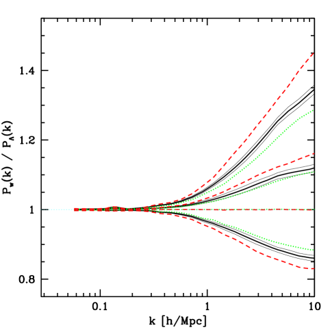
Figure 1: Fractional effect of $w$ on the non-linear mass power spectrum, at fixed linear theory power. The thick lines of a given color/type show, from top to bottom, $w=-0.5,-0.75,-1.5$, all relative to $w=-1$. The black, solid line is for $\Omega_{m}=0.281$, with red, dashed (green, dotted) showing $\Omega_{m}=0.211$ (0.351). Thin black lines show rms statistical error bands (in Figures 1-4, the statistical errors are all similar to these examples).

To minimize the statistical fluctuations, we have used the same initial conditions for simulations with different $w$, except that we adjust the initial amplitude of the perturbations by the factor necessary to produce an identical linear theory density field at $z=0$ (and as a result identical $\sigma_{8}$). All of the figures in this section show results from (110,192,768) simulations. In the next section we investigate the accuracy of the results in detail, finding statistical and numerical convergence to a few percent. Inevitably, the effect of $w$ increases with decreasing $\Omega_{m}$, i.e., increasing dark energy fraction, as shown in the figure. To be clear: in our many figures like this, we are plotting the ratio of power in a model with $w\neq-1$ to a model with $w=-1$, with all the other parameters the same at $z=0$ in both. For example, when we show the result for a different value of $\Omega_{m}$, $\Omega_{m}$ has been changed for both the model in the numerator and the model in the denominator For notational compactness, we will sometimes refer to this type of ratio as $f_{w}(k)\equiv P_{w}(k)/P_{w=-1}(k)$.

To put the 12% (33%) effect of $w=-0.75$ ($w=-0.5$) at $k=10\,h\,{\rm Mpc}^{-1}$ in perspective, we note that the ratio of linear growth of power from early times to $z=0$ between the $w=-1$ and $w=-0.75$ (-0.5) models is $D^{2}(w)/D^{2}(w=-1)=0.83$ (0.57). Note that weak lensing measurements tend to be most sensitive to somewhat smaller $k$ (Huterer & Takada, 2005). On the other hand, Hagan et al. (2005) recently showed that a modification of the power similar in form to ours has a substantial effect on the convergence power over a wide range in $\ell$. Considering the non-trivial $k$ and $z$ dependence, a full parameter forecast calculation (e.g., Simpson & Bridle (2004)) will be needed to see if this effect can change the projections for future weak lensing measurements of $w$ significantly.

We have compared this result to the formula of Ma et al. (1999), and the agreement is not good. The Ma et al. (1999) formula predicts a much larger effect of $w$, with $f_{w=-0.5}(k)$ passing 1.5 at $k=0.4\,h\,{\rm Mpc}^{-1}$, before plateauing at a value of $\sim 2$. This disagreement is not too surprising since Ma et al. (1999) did not use simulations in which $w$ was varied at fixed values of the other parameters. Without a very comprehensive grid of simulations, the simple dependence of the non-linear power on the linear power (and $\Omega_{m}$) could easily be mixed with the type of $w$ dependence that we are studying here. We remind the reader that no rigorous analytic prediction for the non-linear power spectrum exists. The Ma et al. (1999) or Smith et al. (2003) formulas are not derived from first principles – they are physically motivated fitting functions that are used to interpolate/extrapolate simulation results. Even if their basic motivation is perfectly valid, they contain completely free parameters that are only determinable through fits to simulations, so their predictions are only as good as the simulations used to calibrate them. Ma et al. (1999) used only five models, with ($w$, $\sigma_{8}$, $\Omega_{m}$, $h$) = (-1, 1.29, 0.3, 0.75), (-1, 1.53, 0.5, 0.7), (-2/3, ?, 0.4, 0.65), (-1/2, ?, 0.4, 0.65), and (-1/3, ?, 0.45, 0.65). The value of $\sigma_{8}$ was not given for the $w>-1$ simulations, but they were COBE normalized (Bunn & White, 1997), meaning they all have different $\sigma_{8}$. One might hope that this was enough to calibrate the fitting formula everywhere, but this is not at all obvious. It would be very difficult using this set of simulations to disentangle the effects of the different parameters well enough to accurately extrapolate to a point in parameter space not bounded by the set. In particular, a parameter that has a relatively small direct effect will be most difficult to control.

The normalization of the power spectrum, $\sigma_{8}$, also affects the result in a small, qualitatively reasonable way, with increasing $w$ dependence for increasing $\sigma_{8}$, as shown in Figure 2 (the non-linear effect must disappear as $\sigma_{8}\rightarrow 0$).

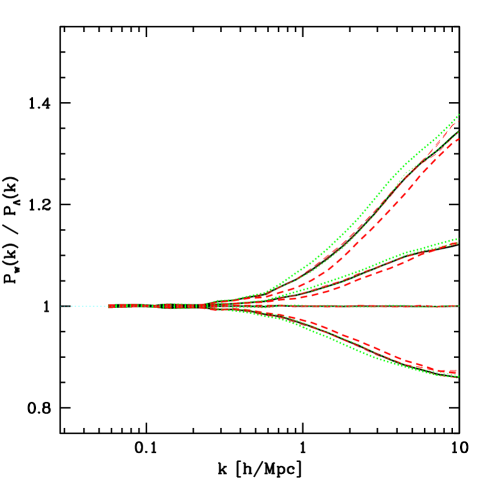
Figure 2: Similar to Figure 1, except thick red, dashed (green, dotted) lines show $\sigma_{8}=0.800$ (0.994). (our central model has $\sigma_{8}=0.897$). Thin lines for variations $\Omega_{b}=0.0462\pm 0.0052$, $h=0.710\pm 0.066$, and $n=0.980\pm 0.065$ are also plotted, to show that they are usually indistinguishable from the central model.

Figure 2 also shows that the changes in the shape of the power spectrum that arise from changes in $\Omega_{b}$, $h$, and $n$ do not change the $w$ dependence significantly.

To explore the origin of the $w$ effect, in Figure 3 we show a similar calculation of the effect of changing $\Omega_{m}\equiv 1-\Omega_{\Lambda}$ while holding the $z=0$ linear power fixed (along with all the other parameters, including $w=-1$).

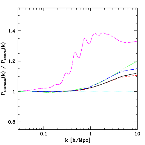
Figure 3: Comparison of the effect of changing $w$ to the effect of changing $\Omega_{m}$, at fixed $z=0$ linear theory power. Black, solid line: our standard ratio of simulated $P_{\rm NL}(k)$ with $w=-0.75$ to $w=-1$. Blue, long-dashed line: ratio of power with $\Omega_{m}=0.192$ to our standard $\Omega_{m}=0.281$ (both with $w=-1$). These two alternative models have identical linear theory power at both $z=24$ and $z=0$. Red, short-dashed line: ratio of power with $\Omega_{m}=0.213$ to standard (this case has linear power equal to the $w=-0.75$ case at $z=1.9$). Green, dotted line: as blue, but based on Smith et al. (2003) (for both numerator and denominator). Magenta, dot-dashed: as blue but based on Ma et al. (1999).

Reducing $\Omega_{m}$ to 0.192 (from 0.281) produces a model with the same power at $z=24$ (our starting redshift) as the model with $w=-0.75$ and $\Omega_{m}=0.281$. We see that the non-linear power in these two models is quite similar. When we match the linear power at $z=1.9$, using $\Omega_{m}=0.213$, the non-linear power is even more similar. It seems likely that Figure 3, and the effect of $w$ in general, could be interpreted in a halo model by accounting for the difference in formation redshift, and thus density profile, of the typical halos dominating the power on the scale of interest (Kuhlen et al., 2005; Huffenberger & Seljak, 2003; Bartelmann et al., 2005; Dolag et al., 2004; Bartelmann et al., 2003, 2002).

The code of Smith et al. (2003) should be able to reproduce this $\Omega_{m}$ dependence. As we see in Figure 3, the agreement is excellent (we can not say for sure that our simulations are accurate enough to believe the $\sim 5$% disagreement at $k=10\,h\,{\rm Mpc}^{-1}$, although they probably are). Note that to make this comparison we have modified the Smith et al. (2003) code to accept an input linear theory power spectrum in place of its usual calculation based on Bond & Efstathiou (1984). The formula of Ma (1998); Ma et al. (1999) does poorly in this test, probably because its $\Omega_{m}$ dependence was essentially calibrated by two simulations with $\Omega_{m}=0.3$, $\sigma_{8}=1.29$, and $\Omega_{m}=0.5$, $\sigma_{8}=1.53$, i.e., far from the combination of parameters we are testing.

Finally, in Figure 4 we show the effect of $w$ on the non-linear power at $z=1.5$, at fixed values of our other parameters.

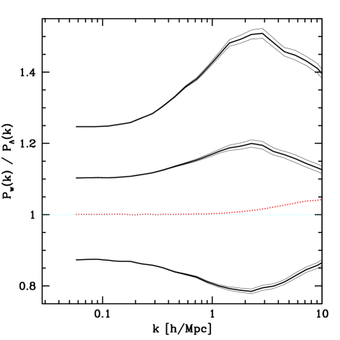
Figure 4: Non-linear power for varying $w$ at $z=1.5$. Thick black (solid) lines are for models with identical linear power and $\Omega_{m}$ at $z=0$ (from top to bottom $w=-0.5$, -0.75, and -1.5, all relative to $w=-1$). Thin black lines show the rms statistical error bands. Note that much of the change here is accounted for by simple differences in linear growth. The red (dotted) line shows $w=-0.5$ relative to $w=-1$ when the two models have been constructed to have identical linear power and $\Omega_{m}(z)$ at $z=1.5$.

Note that in Figure 4 we are comparing models with different linear theory power at the observed redshift, and different $\Omega_{m}(z)$. The difference between $P_{\rm NL}(z=1.5,~{}w=-0.5)$ and $P_{\rm NL}(z=1.5,~{}w=-1)$ at fixed $z=1.5$ linear theory power and $\Omega_{m}(z=1.5)$ is small, so it is not very interesting to plot this, but we show one case, comparing $w=-1.0$ with our usual linear theory power spectrum at $z=0$, but $\Omega_{m}=0.150$, to $w=-0.5$ with $\sigma_{8}$ increased to 1.004, and $\Omega_{m}=0.411$ (these two models have exactly matching linear power and $\Omega_{m}(z)$ at $z=1.5$).

3 Numerical details

In this section we investigate the dependence of our calculations on the numerical parameters of the simulations. Beyond testing the specific results we present, we hope to contribute to the collective wisdom of the research community about how to do precision cosmology based on numerical simulations by exploring the idea of looking at the ratio of power in different models in simulations using identical random numbers for the initial conditions.

For our grid of N-body simulations, we used the PMM code, an improved version of the PM algorithm. It is based on a two-level mesh Poisson solver where the gravitational forces are separated into long-range and short-range components, as described in detail in Trac & Pen (2004) and Merz et al. (2005). The long-range force is computed on the root-level, global mesh, much like in a PM code. To achieve higher spatial resolution, the domain is decomposed into cubical regions and the short-range force is computed on a refinement-level, local mesh. In the current version, PMM can achieve a spatial resolution of 4 times better than a standard PM code at the same cost in memory.

Simulations with $P=192$ and $M=768$ fit conveniently into a single node on the 528-CPU Beowulf cluster at CITA, and run in less than a day. The importance when doing this kind of study of complete freedom to run an arbitrarily large number of exploratory simulations, with relatively quick turn-around, can not be underestimated, so we focus on this configuration. Future precision simulation grids will of course use larger simulations. Our initial guess was that (220, 192, 768) simulations would be most useful, so this section will focus first on the convergence properties of these, including comparisons of (110, 96, 384) to (110, 192, 384), to test the effect of finite particle density at the same force resolution as the (220, 192, 768) simulations, and comparisons of (110, 96, 384) to (110, 96, 768) to test the effect of force resolution. Ultimately, we will conclude that we were overly worried about limited box size and insufficiently worried about limited resolution, so subject to the constraint $P=192$, $M=768$, somewhat smaller box size is optimal (the code we release is based on (110, 192, 768) simulations).

Throughout this section our plots use a standard vertical axis range $0.94-1.06$, to allow easier comparison of the size of different errors.

3.1 Initial conditions

Our transfer functions are computed using the “lingers” code associated with grafic2-1.01 (Bertschinger, 2001). GRAFIC2 is then used to generate the initial conditions. We turn off the GRAFIC2 Hanning window, which isotropizes the small-scale structure at the expense of suppressing the small-scale power.

To determine the linear growth factor (used to convert initial conditions generated for $w=-1$ models into $w\neq-1$ models) we numerically solve

$$D^{\prime\prime}+\frac{3}{2}\left[1-\frac{w(a)}{1+X(a)}\right]\frac{D^{\prime}}{a}-\frac{3}{2}\frac{X(a)}{1+X(a)}\frac{D}{a^{2}}=0$$ (1)

(Linder & Jenkins, 2003), with

$$X(a)=\frac{\Omega_{m}}{1-\Omega_{m}}e^{-3\int_{a}^{1}d\ln a^{\prime}w(a^{\prime})}~{}.$$ (2)

When we compare simulations with the same box size but different particle density, the initial conditions of the box with fewer particles are set by a sharp $k$-space filter applied to the initial conditions of the higher resolution box. This is equivalent to simply regenerating the initial conditions with the same random numbers for the large-scale modes (for our method of generating initial conditions), but not equivalent to re-binning the density and momentum fields in real space (the latter method introduces a suppression of high-$k$ power that increases the level of disagreement between the results for the two particle densities).

3.2 Starting redshift

It is important for precision calculations to test the affect of changing the starting redshift in the simulations. This can identify, for example, transients due to the imperfection of the Zel’Dovich (1970) approximation (Scoccimarro, 1998). Figure 5 shows the change in the effect of $w$ as we increase the starting redshift, $z_{\rm i}$, from our standard $z_{\rm i}=24$.

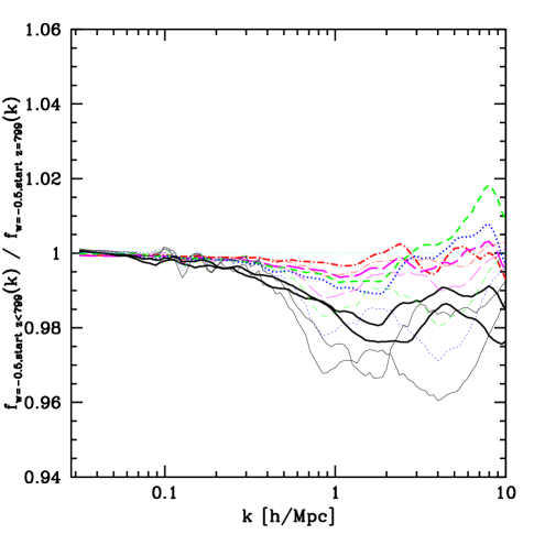
Figure 5: Change in the effect of $w$, $f_{w=-0.5}(k)\equiv P_{w=-0.5}(k)/P_{w=-1}$, with starting redshift in the simulations. Thick (thin) lines are power at $z=0$ ($z=1.5$). The denominator is for starting $z_{\rm i}=799$, with black/solid showing the difference for $z_{\rm i}=24$, blue/dotted $z_{\rm i}=49$, green/short-dashed $z_{\rm i}=99$, magenta/long-dashed $z_{\rm i}=199$, and red/dot-dashed $z_{\rm i}=399$. The two black lines of each type show different realizations of the initial conditions.

Note that it is not automatically the case that higher $z_{\rm i}$ is better, because numerical errors (most obviously suppression of power by limited force resolution) have more time to accumulate in that case. The agreement is good but not perfect, with errors as large as 2% at $z=0$ and $\sim 3$% at $z=1.5$. Subsequent to our runs for this paper, we found a small problem in the PMM force kernel which leads to this disagreement – it is not serious so we leave the more accurate calculation for the future.

3.3 Mass resolution

Figure 6(a) shows the effect of varying the number of particles, for a fixed force resolution, by comparing the average of two (110, 96, 384) simulations to the average of two (110, 192, 384) simulations (the pairs have different random initial conditions).

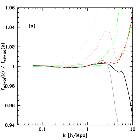
Figure 6: Change in the effect of $w$, $f_{w=-0.5}(k)\equiv P_{w=-0.5}(k)/P_{w=-1}$, with number of particles. Thick (thin) lines are power at $z=0$ ($z=1.5$), with $L=110\,h^{-1}\,{\rm Mpc}$ (a) or $L=55\,h^{-1}\,{\rm Mpc}$ (b) and force mesh $M=384$. The numerator is simulations with $(P=96)^{3}$ particles, the denominator is $P=192$. Red (dashed) lines include subtraction of Poisson noise $P_{\rm noise}(k)=(L/P)^{3}$, black (solid) do not. For reference, the green (dotted) lines show $1+P_{\rm noise}(k)/P_{\rm measured}(k)$, where $P_{\rm measured}(k)$ is the measured power for the $w=-1$ model (after deconvolution of the power spectrum measurement mesh, but without noise subtraction). The two green lines of each thickness represent the two particle densities. The vertical cyan (dotted) lines mark $k=(96,192)\pi/110\,h^{-1}\,{\rm Mpc}$.

Note that this is a test of the effect of adding high $k$ power in the initial conditions in addition to the effect of simply subdividing the mass. We have done the same comparison with a factor of two better force resolution and the results are similar. We see that for a (110, 96, 384) simulation at $z=0$, limited particle density becomes a $\tilde{>}2$% problem only at $k\tilde{>}8\,h\,{\rm Mpc}^{-1}$. At $z=1.5$ it is a more serious problem, surpassing 3% at $k\simeq 4\,h\,{\rm Mpc}^{-1}$ and quickly diverging (although note the expanded axis scale – the error is actually only 15% at $k=10\,h\,{\rm Mpc}^{-1}$).

A potential solution to this problem is to subtract, after correcting for the mass assignment smoothing, Poisson shot-noise power $P_{\rm noise}(k)=\bar{n}^{-1}$, where $\bar{n}=(P/L)^{3}$ is the mean particle density (Baugh & Efstathiou, 1994; Baugh et al., 1995); however, as others have noted (Baugh et al., 1995; Smith et al., 2003; Sirko, 2005), the idea that the effect of finite particle density is to add this white noise component is only a guess, not something that can be assumed to hold, and in fact it is known not to hold at early times for a uniform grid start. Figure 6 calls into question the idea that subtracting white shot-noise is ever useful for high precision calculations. (See Figure 11 of Sirko (2005) for an enlightening plot of the evolution of the particle discreteness power starting from a fixed grid – we produced a similar figure, but Sirko (2005)’s is similar enough that it is not worth including ours in this paper.) Note that when we say that subtracting Poisson noise is not useful for high precision calculations, this does not mean it never leads to an improvement in accuracy – it sometimes does – the problem is that there is no clearly identifiable regime where the correction is both significant and accurate enough for high precision work. This should probably be regarded as a well-known fact (e.g., Baugh et al. (1995) conclude that the discreteness corrections they discuss can not be applied consistently, and simply resort to using enough particles to make them negligible), but it is worth reiterating. It seems unlikely that a glass start (Smith et al., 2003) will lead to perfectly stable, non-interacting, discreteness power either. Ultimately, direct tests of the convergence of observable statistics with increasing particle density for different methods of setting up the initial conditions (Smith et al., 2003; Joyce et al., 2004; Sirko, 2005), and possibly different methods for correcting for discreteness, are the only way to determine which method works best.

Figure 6(b) shows the same comparison as Figure 6(b), reduced in scale by a factor of two, i.e., (55, 96, 384) is compared to (55, 192, 384), to estimate the accuracy of a (110, 192, 768) simulation (there is some noise in this comparison so we have averaged two realizations of each size simulation). The results are much better, with accuracy better than 2% at $z=0$, and better than 4% for $z=1.5$ (better than 2% for $k\tilde{<}6\,h\,{\rm Mpc}^{-1}$). Note that the apparent helpfulness of Poisson noise subtraction at $z=1.5$ is probably coincidental, as it quickly becomes an over-correction at $k>10\,h\,{\rm Mpc}^{-1}$.

Our default in this paper is to not subtract shot noise.

3.4 Force resolution

Figure 7 shows the effect of increasing the force mesh resolution, for a fixed number of particles.

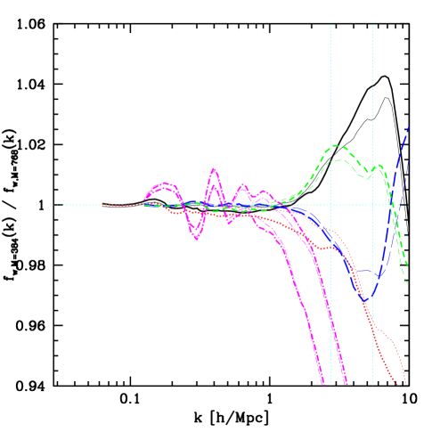
Figure 7: Change in the effect of $w$, $f_{w=-0.5}(k)\equiv P_{w=-0.5}(k)/P_{w=-1}$, with force resolution. Black/solid (red/dotted) lines are power at $z=0$ ($z=1.5$) in $L=110\,h^{-1}\,{\rm Mpc}$ simulations with $(P=96)^{3}$ particles (thick lines) or $P=192$ (thin lines). The denominator is for mesh $M=768$, with numerator $M=384$. The blue/long-dashed (green/short-dashed) lines show the same comparisons for $L=55\,h^{-1}\,{\rm Mpc}$ simulations (the effect appears to change sign, i.e., the curves are not mislabeled). For reference, magenta/dot-dashed lines show the ratio of power spectra [i.e., simply $P(k)$, not $f_{w}(k)$] for $w=-1$, comparing $M=384$ to $M=768$, for an $L=55\,h^{-1}\,{\rm Mpc}$ box with $P=96$ (thick) or $P=192$ (thin) (the poorer agreement in each case is $z=0$, better is $z=1.5$). The vertical cyan/dotted lines show $k=(96,192)\pi/110\,h^{-1}\,{\rm Mpc}$.

Comparing $L=110\,h^{-1}\,{\rm Mpc}$ simulations with $(M=384)^{3}$ force mesh cells to $M=768$, we see that the error on the former is as large as 4% at $z=0$ and 7% at $z=1.5$. The errors fall to $<3$% for a similar comparison using $L=55\,h^{-1}\,{\rm Mpc}$ boxes. In Figure 7, we break from our general policy of plotting only ratios of different models to show the lack of convergence of the absolute power spectrum, $P_{M=384}(k)/P_{M=768}(k)$. This shows the value of computing ratios – the better than 3% agreement in $f_{w=-0.5}(k)$ for the two meshes occurs in spite of a suppression of the absolute power by as much as 36%.

3.5 Box size

Insufficient box size can cause two problems: simple random fluctuations around the mean of a statistic due to limited volume, i.e., sample variance; and systematic errors in the mean of a statistic due to missing couplings to large-scale modes (or even small-scale modes missing due to limited $k$-resolution). The first of these can be eliminated by averaging over sufficient realizations of the initial conditions while the second can not (although various methods have been proposed to improve the results, e.g., Sirko (2005)). Bagla & Ray (2005) discuss requirements on simulation box size, but not for the power spectrum – note that the requirements on numerical parameters will generally be different for different statistics (one advantage of the power spectrum is that it is not directly sensitive to structure on scales larger than the box).

Figure 8 shows that a single $L=220~{}\,h^{-1}\,{\rm Mpc}$ simulation is sufficient to compute the fractional difference in power between $w=-0.5$ and $w=-1$ to better than 1% rms statistical error. A single $L=110~{}\,h^{-1}\,{\rm Mpc}$ simulation would achieve about 2% precision at $z=0$ and 3% at $z=1.5$.

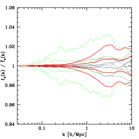
Figure 8: Level of random fluctuations in the fractional effect of $w$ on the non-linear power. Black, thin lines show $f_{w=-0.5}(k)$ from $L=220\,h^{-1}\,{\rm Mpc}$ simulations with nine different random seeds, each divided by the average of $f_{w=-0.5}(k)$ over all nine, at $z=0$. The inner thick red/solid (green/dotted) lines show bin-by-bin the standard deviation of the nine around their mean (i.e., the error when using a single realization) at $z=0$ ($z=1.5$). The outer thick lines are the same but for $L=110\,h^{-1}\,{\rm Mpc}$ simulations.

In principle this Figure can be sensitive to the binning in $k$ but in practice it is not because the errors in nearby bins are strongly correlated.

Figure 9 addresses the systematic error possibility by comparing $L=440\,h^{-1}\,{\rm Mpc}$, $220\,h^{-1}\,{\rm Mpc}$, and $110\,h^{-1}\,{\rm Mpc}$ boxes, with the power in each case averaged over 9 realizations with different seeds.

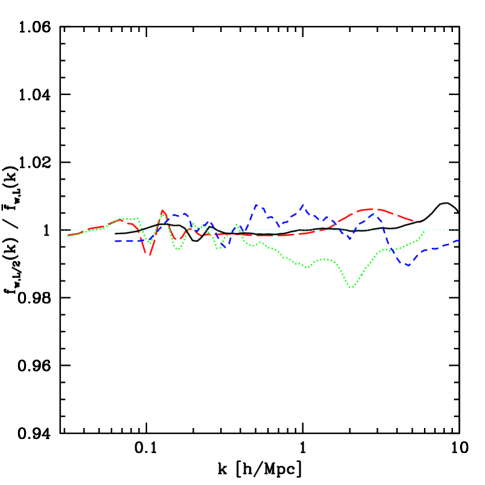
Figure 9: Effect of box size on the fractional effect of $w$ on the non-linear power. The black/solid (blue/short-dashed) line shows at $z=0$ ($z=1.5$) the ratio of $f_{w=-0.5}(k)$ computed by averaging over nine $L=110\,h^{-1}\,{\rm Mpc}$ simulations to the result from $L=220\,h^{-1}\,{\rm Mpc}$ simulations similarly averaged. The red/long-dashed (green/dotted) line shows at $z=0$ ($z=1.5$) similar ratios for $L=220\,h^{-1}\,{\rm Mpc}$ compared to $L=440\,h^{-1}\,{\rm Mpc}$. Note that different sized simulations do not have matching grids in $k$, so these comparisons involve some interpolation.

Remarkably, there is no significant sign of systematic error, even in the $L=110\,h^{-1}\,{\rm Mpc}$ calculation (the error in the absolute power is larger). The maximum disagreement in Figure 9, $<2$% between the $L=440\,h^{-1}\,{\rm Mpc}$ and $L=220\,h^{-1}\,{\rm Mpc}$ simulations at $z=1.5$, appears not to be strictly a boxsize effect at all, but rather a coupling between boxsize and limited particle density (the particle noise appears to whiten more quickly in the larger box). For these comparisons we have matched the particle density and force resolution between the two box sizes, i.e., we compare (440, 192, 768) to (220, 96, 384), and (220, 192, 768) to (110, 96, 384).

3.6 Time steps

For our main grid we used $\sim 210$ time steps to evolve the simulations ($\sim 120$ for $0.0<z<1.5$). Reducing this to $\sim 80$ ($\sim 30$) leads to the $<1$% change shown in Figure 10.

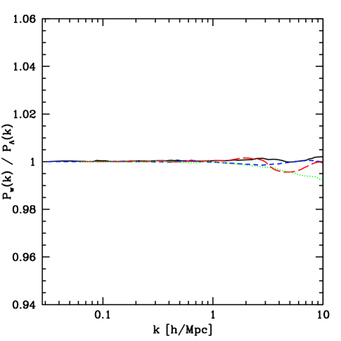
Figure 10: Effect of time step size on the fractional effect of $w$ on the non-linear power. The black/solid (blue/short-dashed) line shows at $z=0$ ($z=1.5$) the ratio of $f_{w=-0.5}(k)$ computed from (220, 192, 768) simulations with $\sim 80$ time steps ($\sim 30$ for $0.0<z<1.5$) to $\sim 210$ ($\sim 120$) time steps. The red/long-dashed (green/dotted) line shows the same comparison for (110, 192, 768) simulations.

It appears that we could accelerate our grid calculation by a factor of a few by relaxing our standard time step restrictions.

3.7 Power spectrum computation

We generally use an $(N=1024)^{3}$ grid for the power spectrum computation, with a simple correction for the CIC smoothing, which we see in Figure 11 is essentially exact (better than 0.5% as tested using measurements with different $N$) out to $\sim 0.7~{}k_{\rm Nyq}$, where $k_{\rm Nyq}\equiv\pi N/L$ (see Jing (2004) for a discussion of aliasing).

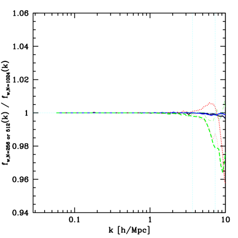
Figure 11: Change in effect of $w$, $f_{w=-0.5}(k)\equiv P_{w=-0.5}(k)/P_{w=-1}$, when we change the resolution of the grid that we use to compute the power spectrum for $L=110\,h^{-1}\,{\rm Mpc}$ simulations. The denominator is always power computed using $(N=1024)^{3}$ cells. For $P=192$, $M=768$, black (solid) show the change for $N=512$ and red (dotted) $N=256$, while for $P=96$, $M=384$ we use blue (long-dashed) and green (short-dashed) to show the same two $N$’s, respectively. The thick lines show $z=0$, thin lines show $z=1.5$. The vertical cyan (dotted) lines mark $(128,256)\pi/L$.

Note that if we are looking at a simple ratio of raw power in two simulations of the same size, the CIC smoothing correction we apply has no effect, because it is multiplicative (assuming we are not subtracting shot-noise). Figure 11 shows that a grid spacing $\Delta x\sim 0.2~{}\,h^{-1}\,{\rm Mpc}$ is sufficient to introduce essentially no error into our computation at $k<10~{}\,h\,{\rm Mpc}^{-1}$, independent of the particle density.

4 Simulation grid and fitting formula

Our limited quantitative goal in this paper is to provide a module that can be grafted onto Smith et al. (2003) to account for varying $w$.

We found in §3 that to reduce finite particle density and force resolution errors to 2-3%, we need resolution equivalent to (110, 192, 768). An $L=110\,h^{-1}\,{\rm Mpc}$ box is sufficient to achieve percent level systematic accuracy, and $\sim 3$% statistical precision, i.e., (110, 192, 768) simulations are sufficient to essentially solve the problem of computing the effect of $w$ to a few percent, especially if we average over a few different realizations of the initial conditions, and considering that the maximum errors are generally near $10\,h\,{\rm Mpc}^{-1}$, where baryons probably limit our precision anyway. The code we describe in this section is based on a grid of (110, 192, 768) simulations, averaged over four realizations of the initial conditions for each grid point. At this point it would be straightforward to perform a grid of larger simulations to meet the numerical requirements more comfortably, but given the generally limited scope of this paper, we have deferred this to future work.

Our grid of models is motivated by the idea of Taylor expanding the dependence of $P_{\rm NL}(w)/P_{\rm NL}(w=-1)$ on the other parameters around a central model. The central model and positive and negative variations are $\sigma_{8}=0.897\pm 0.097$, $\Omega_{m}=0.281\pm 0.070$, $\Omega_{b}=0.0462\pm 0.0052$, $h=0.710\pm 0.066$, and $n=0.980\pm 0.065$ (motivated by the best fit and $3\sigma$ errors from Seljak et al. (2005)) To be clear: we are only varying these parameters individually, not in combinations, i.e., the grid does not have $3^{N}$ points. For the two most important parameters, $\Omega_{m}$ and $\sigma_{8}$, we add the four possible joint variations to the grid. For each variation of the non-$w$ parameters, we run models with $w=$-0.5, -0.75, -1.0, and -1.5. We extract the power spectrum at $z=$1.5, 1.0, 0.5, 0.25, and 0.0. We do not advocate this kind of grid for a more general simulation project, where a set of simulations guided by CMB constraints should be most efficient (White & Vale, 2004).

It would probably be straightforward to extend Smith et al. (2003) by modifying their fitting functions $f_{i}(\Omega_{m})$ to depend on $w$, but we take the less sophisticated approach of describing the change in power relative to $w=-1$ by a multi-polynomial function of the cosmological parameters. If $\mathbf{p}$ is the vector of cosmological parameters, which we take to include $z$, the formula for the correction factor is

$$\ln\left[\frac{P_{\rm NL}(w)/D^{2}(w)}{P_{\rm NL}(w=-1)/D^{2}(w=-1)}\right](k,\mathbf{p}) =$$ (3)

$$\left(\prod_{i=1}^{N_{p}}\sum_{\nu_{i}=0}^{N_{i}}p_{i}^{\nu_{i}}\right)A_{\nu_{1}\nu_{2}\nu_{3}...\nu_{N_{p}}}(k)$$ ,

where $N_{p}$ is the number of cosmological parameters, $N_{i}$ is the order of polynomial to use for each of them, and $A_{\nu_{1}\nu_{2}\nu_{3}...\nu_{N_{p}}}(k)$ are coefficients to be determined by a least-squares fit to simulations. $D(w)$ is the linear growth factor, normalized to 1 at $z=0$ (we divide out the growth factor in Equation 4 to remove the relatively trivial linear evolution with redshift). Note that this formula includes many cross-terms for which we do not have simulations in our grid – their coefficients are set to zero when the fit is performed using singular value decomposition (we use Equation 4 because it is easy to write down and implement in code, and extends automatically when additional simulations become available). We measure $P_{\rm NL}(k)$ from the simulations in bands spaced by $\Delta\log_{10}k=0.1$, and determine a separate set of $A$s for each band. Once the $A$s are determined, $P_{\rm NL}$ for any model is computed by simply plugging the desired parameters into Equation 4 and multiplying the result by the non-linear power in the corresponding $w=-1$ model, and the appropriate linear growth factors. Our code quantifying the results, with an example showing how to use it, can be found at http://www.cita.utoronto.ca/$\sim$pmcdonal/code.html, under the name “wcorrector.” This code is only tested for $k<10\,h\,{\rm Mpc}^{-1}$. The user who needs to integrate to higher $k$ should absorb the uncertainty in the extrapolation into the uncertainty they are assuming from baryon effects.

Note that we have not separated the dependence of the non-linear power on $\Omega_{m}$ through its effect on past non-linear growth from its effect through the transfer function (except in Figure 3). Separating these would probably be useful in the future, so that formulas can be used with arbitrary linear power spectrum without fear that spurious effects of $\Omega_{m}$ will be generated. However, because we have used fully accurate transfer functions from “lingers” (Bertschinger, 2001), the coupling between the two influences of $\Omega_{m}$ can have no effect on calculations within the standard $\Lambda$CDM model. Additionally, we showed that the effect of changing the power spectrum shape on $f_{w}$ at fixed $\sigma_{8}$ is negligible, so it can probably be safely assumed that the effect of $\Omega_{m}$ that we see is coming through the past growth.

The reader may ask whether a more thoughtful, theoretically motivated fitting formula could be more general and efficient. This is possible. On the other hand, a drawback of such formulas is that they trap the user into a limited functional form for the various dependences. When a carefully constructed fitting formula is found not to fit to the required level of precision, it is not generally straightforward to extend it. It is simple to extend Equation 4 to fit any set of simulations. Furthermore, as we saw in the case of the Ma et al. (1999) formula, it is easy in these cases to be deceived into thinking that they are more generally applicable than they really are, i.e., to think of them as having genuine predictive power rather than simply being a method of interpolation between simulation results. Equation 4 makes the interpolatory nature of these fitting formulas explicit. Ultimately, a hybrid approach may be optimal. A physically motivated fitting formula could be used to remove much of the gross parameter dependence, with a general formula like Equation 4 used to make corrections for the imperfections in the fitting formula. The hope would be that this would allow a sparser calibration grid than would otherwise be needed.

5 Conclusions

We have isolated the effect of changing $w$ on the non-linear power spectrum of mass density fluctuations by comparing simulations with identical linear theory density fields at the observed redshift. We focused on this definition of the effect of $w$ (i.e., fixed linear theory power and other parameters at $z=0$) simply because it has not been carefully considered in the past, and this complements predictive formulas calibrated only for $w=-1$ (e.g., Smith et al. (2003)). The change in power relative to $w=-1$ is $\tilde{<}10$% for $k<1\,h\,{\rm Mpc}^{-1}$ (for $-0.5<w<-1.5$), but rises to 12% by $k=10\,h\,{\rm Mpc}^{-1}$ in a model with $w=-0.75$, and $\sim 33$% for $w=-0.5$ (at $z=0$). Among the other cosmological parameters, the size of the effect is primarily sensitive to the dark energy fraction, i.e., $\Omega_{m}$ in flat models. The power spectrum normalization (i.e., $\sigma_{8}$) also has a small effect, but the slope/shape of the power spectrum are irrelevant (as represented by varying $n$, $\Omega_{b}$, and $h$ at fixed $\sigma_{8}$).

Figure 3 confirms the accuracy of the formula of Smith et al. (2003) for the dependence on $\Omega_{m}$ in $\Lambda$CDM models, at least once it has been modified to use high accuracy transfer functions.

We provide a simple code (http://www.cita.utoronto.ca/$\sim$pmcdonal/code.html) quantifying the effect of $w$ as a function of $k$, $z$, $w$, $\Omega_{m}$, $\sigma_{8}$, $n$, $h$, and $\Omega_{b}$, to be used as a correction to $P_{\rm NL}(k)$ calculations accurate at $w=-1$. The dependence of the power spectrum on $w$ should be accurate to a few percent for $k\tilde{<}10~{}\,h\,{\rm Mpc}^{-1}$. Our quantitative results may be useful for making more realistic projections of the future potential to measure $w$ by methods sensitive to the non-linear power (primarily weak lensing). Our code will be appropriate for forecasts of parameter measurements from future large data sets, or parameter determinations using data sets that at least include WMAP. It should be used cautiously for fits to limited amounts of weak lensing data alone, since we do not cover extreme parameter values (however, by construction the code will only be unreliable in regions of parameter space that are ruled out by other observations).

Our ambitions have been quite limited in this paper. We have not tried to determine the absolute power in the central model because that is much more difficult to simulate precisely than the fractional changes we studied here, requiring both larger box sizes and higher resolution. Much of the error caused by limitations in the simulations cancels when we take ratios of power spectra, a fact that should make future construction of high precision grids of simulation predictions easier.

References

- Abazajian et al. (2004) Abazajian K. et al., 2004, ArXiv Astrophysics e-prints, arXiv:astro-ph/0408003
- Bagla & Ray (2005) Bagla J. S., Ray S., 2005, MNRAS, 232
- Bartelmann et al. (2005) Bartelmann M., Dolag K., Perrotta F., Baccigalupi C., Moscardini L., Meneghetti M., Tormen G., 2005, New Astronomy Review, 49, 199
- Bartelmann et al. (2002) Bartelmann M., Perrotta F., Baccigalupi C., 2002, A&A, 396, 21
- Bartelmann et al. (2003) Bartelmann M., Perrotta F., Baccigalupi C., 2003, A&A, 400, 19
- Baugh & Efstathiou (1994) Baugh C. M., Efstathiou G., 1994, MNRAS, 270, 183
- Baugh et al. (1995) Baugh C. M., Gaztanaga E., Efstathiou G., 1995, MNRAS, 274, 1049
- Benabed & Bernardeau (2001) Benabed K., Bernardeau F., 2001, Phys. Rev. D, 64, 083501
- Benabed & Van Waerbeke (2003) Benabed K., Van Waerbeke L., 2003, ArXiv Astrophysics e-prints, arXiv:astro-ph/0306033
- Bertschinger (2001) Bertschinger E., 2001, ApJS, 137, 1
- Bond & Efstathiou (1984) Bond J. R., Efstathiou G., 1984, ApJ, 285, L45
- Bunn & White (1997) Bunn E. F., White M., 1997, ApJ, 480, 6
- Dolag et al. (2004) Dolag K., Bartelmann M., Perrotta F., Baccigalupi C., Moscardini L., Meneghetti M., Tormen G., 2004, A&A, 416, 853
- Eisenstein et al. (2005) Eisenstein D. J. et al., 2005, ArXiv Astrophysics e-prints, arXiv:astro-ph/0501171
- Hagan et al. (2005) Hagan B., Ma C., Kravtsov A. V., 2005, ArXiv Astrophysics e-prints, arXiv:astro-ph/0504557
- Heitmann et al. (2004) Heitmann K., Ricker P. M., Warren M. S., Habib S., 2004, ArXiv Astrophysics e-prints, astro-ph/0411795
- Huffenberger & Seljak (2003) Huffenberger K. M., Seljak U., 2003, MNRAS, 340, 1199
- Huterer & Takada (2005) Huterer D., Takada M., 2005, Astroparticle Physics, 23, 369
- Jarvis et al. (2005) Jarvis M., Jain B., Bernstein G., Dolney D., 2005, ArXiv Astrophysics e-prints, astro-ph/0502243
- Jing (2004) Jing Y. P., 2004, ArXiv Astrophysics e-prints, astro-ph/0409240
- Joyce et al. (2004) Joyce M., Levesque D., Marcos B., 2004, ArXiv Astrophysics e-prints, astro-ph/0411607
- Klypin et al. (2003) Klypin A., Macciò A. V., Mainini R., Bonometto S. A., 2003, ApJ, 599, 31
- Knop et al. (2003) Knop R. A. et al., 2003, ApJ, 598, 102
- Knox et al. (2005) Knox L., Song Y. ., Tyson J. A., 2005, ArXiv Astrophysics e-prints, astro-ph/0503644
- Kuhlen et al. (2005) Kuhlen M., Strigari L. E., Zentner A. R., Bullock J. S., Primack J. R., 2005, MNRAS, 357, 387
- Linder & Jenkins (2003) Linder E. V., Jenkins A., 2003, MNRAS, 346, 573
- Ma (1998) Ma C., 1998, ApJ, 508, L5
- Ma et al. (1999) Ma C., Caldwell R. R., Bode P., Wang L., 1999, ApJ, 521, L1
- Merz et al. (2005) Merz H., Pen U., Trac H., 2005, New Astronomy, 10, 393
- Peacock & Dodds (1996) Peacock J. A., Dodds S. J., 1996, MNRAS, 280, L19
- Ratra & Peebles (1988) Ratra B., Peebles P. J. E., 1988, Phys. Rev. D, 37, 3406
- Riess et al. (2004) Riess A. G. et al., 2004, ApJ, 607, 665
- Scoccimarro (1998) Scoccimarro R., 1998, MNRAS, 299, 1097
- Seljak et al. (2005) Seljak U. et al., 2005, Phys. Rev. D, 71, 103515
- Seljak & Zaldarriaga (1996) Seljak U., Zaldarriaga M., 1996, ApJ, 469, 437
- Simpson & Bridle (2004) Simpson F., Bridle S., 2004, ArXiv Astrophysics e-prints, astro-ph/0411673
- Sirko (2005) Sirko E., 2005, ArXiv Astrophysics e-prints, astro-ph/0503106
- Smith et al. (2003) Smith R. E. et al., 2003, MNRAS, 341, 1311
- Tegmark et al. (2004) Tegmark M. et al., 2004, Phys. Rev. D, 69, 103501
- Trac & Pen (2004) Trac H., Pen U., 2004, New Astronomy, 9, 443
- Vale & White (2003) Vale C., White M., 2003, ApJ, 592, 699
- White (2004) White M., 2004, Astroparticle Physics, 22, 211
- White & Vale (2004) White M., Vale C., 2004, Astroparticle Physics, 22, 19
- Zel’Dovich (1970) Zel’Dovich Y. B., 1970, A&A, 5, 84
- Zhan (2004) Zhan H., 2004, Ph.D. Thesis
- Zhan & Knox (2004) Zhan H., Knox L., 2004, ApJ, 616, L75