Reconnection at the Heliopause

Abstract

In this MHD-model of the heliosphere, we assume a Parker–type flow, and a Parker–type spiral magnetic field, which is extrapolated further downstream from the termination shock to the heliopause. We raise the question whether the heliopause nose region may be leaky with respect to fields and plasmas due to nonideal plasma dynamics, implying a breakdown of the magnetic barrier. We analyse some simple scenarios to find reconnection rates and circumstances, under which the heliosphere can be an ”open” or a ”closed” magnetosphere. We do not pretend to offer a complete solution for the heliosphere, on the basis of nonideal MHD theory, but present a prescription to find such a solution on the basis of potential fields including the knowledge of neutral points. As an example we imitate the Parker spiral as a monopole with a superposition of homogeneous asymptotical boundary conditions. We use this toy model for $x<-R$ where $R=100$ AU is the distance of the termination shock to describe the situation in the nose region of the heliopause.

,

1 Introduction

In the past several calculations concerning the role of magnetic reconnection in the vicinity of the heliopause have been performed. Fahr et al. (1986)(and references therein) calculated reconnection probabilities and gave estimations for reconnection rates, but without complete reconnection solutions of the nonideal MHD equations. Here, we present a plane model of the heliosphere in the framework of stationary nonideal MHD. We assume that the tail direction is the direction of the $x$–axis (see Figure 1), which is also the direction of the asymptotical flow around the heliosphere. The direction of invariance is the $z$–direction. Results depend mainly on the tilt angle between the asymptotical magnetic field to the asymptotical plasma velocity. We concentrate on investigating the region where the interstellar plasma encounters the solar wind plasma.

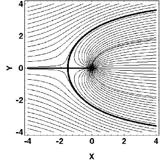
Figure 1: The heliospheric outflow in the vicinity of the stagnation point, similar to the classical Parker outflow. The scale is given in units of 100 AU

2 Stationary nonideal MHD–flows in 2D

2.1 Basic equations

In our plane model of the heliosphere we make the following assumptions:

• we take only stationary fields, i.e. $\partial/\partial t=0$, and take: $\partial/\partial z=0$

• incompressibility as a substitute for the energy equation is assumed. Incompressibility here means that the density of a fluid element moving with the flow does not change in time meaning that the convective derivative $\frac{d\rho}{dt}:=\frac{\partial\rho}{\partial t}+\vec{v}\cdot\vec{\nabla}\rho$ vanishes. Using the mass continuity $\frac{\partial\rho}{\partial t}+\vec{\nabla}\cdot(\rho\vec{v})=0$ we thus can derive with $\frac{d\rho}{dt}=-\rho\vec{\nabla}\cdot\vec{v}=0$ which implies $\vec{\nabla}\cdot\vec{v}=0$ and $\vec{v}\cdot\nabla\rho=0$. Then we introduce the auxiliary flow field or streaming vector $\vec{w}$ with $\vec{w}=\sqrt{\rho}\,\vec{v}\quad$leading to $\nabla\cdot\vec{w}=0$.

Therefore, the basic MHD equations are given by the following set

$$\vec{\nabla}\cdot\vec{B} = 0$$ (1)

$$\vec{w}: = \sqrt{\rho}\,\vec{v}$$ (2)

$$\vec{\nabla}\cdot\vec{w} = 0$$ (3)

$$\vec{\nabla}\times\vec{B} = \mu_{0}\,\vec{j}$$ (4)

$$-\vec{\nabla}\phi_{e}+E_{0}\vec{e}_{z}+\frac{1}{\sqrt{\rho}}\vec{w}\times\vec{B} = \vec{R}$$ (5)

$$\vec{\nabla}\left(\frac{1}{2}\vec{w}^{2}+p\right) = \frac{1}{\mu_{0}}\left(\vec{\nabla}\times\vec{B}\right)\times\vec{B}-\left(\vec{\nabla}\times\vec{w}\right)\times\vec{w}$$ (6)

where $p$ is the thermal pressure and $p+\frac{1}{2}\vec{w}^{2}=\Pi$ is the Bernoulli pressure. $\phi_{e}(x,y)$ is the part of the electric potential whose gradient gives the poloidal field components (i.e. the components in $x$- and $y$-direction) of the electric field, so that $\vec{E}=-\vec{\nabla}\phi_{e}(x,y)+E_{0}\vec{e}_{z}$, and $E_{0}$ is a constant component of the electric field in the invariant $z$–direction. This is to ensure that $\vec{\nabla}\times\vec{E}=-\frac{\partial\vec{B}}{\partial t}=0$ (stationarity condition) and to fulfill $\frac{\partial\vec{E}}{\partial z}=0$. $\vec{R}$ is the nonidealness and the other symbols have their usual meaning. Eq. (5) is the generalized Ohm’s law (see Vasyliunas (1972) and Hesse & Schindler (1988)). For $\vec{w}$ and $\vec{B}$ we make the following ansatz:

$$\vec{w} = \vec{\nabla}\zeta\times\vec{e}_{z}+w_{z}\vec{e}_{z}\equiv\vec{w}_{p}+w_{z}\vec{e}_{z}$$ (7)

$$\vec{B} = \vec{\nabla}\alpha\times\vec{e}_{z}+B_{z}\vec{e}_{z}\equiv\vec{B}_{p}+B_{z}\vec{e}_{z}$$ (8)

where the index p on the right hand side of these equations stands for the poloidal part of the magnetic and the velocity field, and $\zeta$, $\alpha$, $B_{z}$, and $w_{z}$ are functions of $x$ and $y$. With these assumptions we find for the generalized Ohm’s law from Eq. (5)

$$\vec{w}\times\vec{B}=(\vec{\nabla}\zeta\times\vec{e}_{z}+w_{z}\vec{e}_{z})\times(\vec{\nabla}\alpha\times\vec{e}_{z}+B_{z}\vec{e}_{z})$$ (9)

which results in

$$\!\!\!\!\!\!\!\!\!\!\!-(\vec{\nabla}\zeta,\vec{e}_{z},\vec{\nabla}\alpha)\vec{e}_{z}-B_{z}\vec{\nabla}\zeta+w_{z}\vec{\nabla}\alpha=\sqrt{\rho}\left(\frac{\partial\phi_{e}}{\partial\alpha}\vec{\nabla}\alpha+\frac{\partial\phi_{e}}{\partial\zeta}\vec{\nabla}\zeta+\vec{R}-E_{0}\vec{e}_{z}\right)$$ (10)

The momentum balance equation Eq. (6) can be written as

$$\vec{\nabla}\Pi = -\frac{1}{\mu_{0}}\Delta\alpha\vec{\nabla}\alpha+\frac{1}{\mu_{0}}(\vec{\nabla}B_{z}\times\vec{e}_{z})\times(\vec{\nabla}\alpha\times\vec{e}_{z})-\frac{1}{\mu_{0}}B_{z}\vec{\nabla}B_{z}$$ (11)

$$+\Delta\zeta\vec{\nabla}\zeta+\left(\vec{\nabla}w_{z}\times\vec{e}_{z}\right)\times\left(\vec{\nabla}\zeta\times\vec{e}_{z}\right)+w_{z}\vec{\nabla}w_{z}$$

$$= -\frac{1}{\mu_{0}}\Delta\alpha\vec{\nabla}\alpha-\frac{1}{\mu_{0}}(\vec{\nabla}B_{z},\vec{e}_{z},\vec{\nabla}\alpha)\vec{e}_{z}-\frac{1}{\mu_{0}}B_{z}\vec{\nabla}B_{z}$$

$$+\Delta\zeta\vec{\nabla}\zeta+(\vec{\nabla}w_{z},\vec{e}_{z},\vec{\nabla}\zeta)\vec{e}_{z}+w_{z}\vec{\nabla}w_{z}$$

The problem here is to get rid of the $z$–component on the right hand side of equation (11), as the $z$-dependence of the Bernoulli pressure $\Pi$ has to vanish if the problem should be restricted to a two–dimensional problem. This can be solved by setting

$$\vec{0}\stackrel{{\scriptstyle!}}{{=}} (\vec{\nabla}w_{z},\vec{e}_{z},\vec{\nabla}\zeta)\vec{e}_{z}-\frac{1}{\mu_{0}}(\vec{\nabla}B_{z},\vec{e}_{z},\vec{\nabla}\alpha)\vec{e}_{z}$$ (12)

$$\Longrightarrow\quad\vec{0}= \vec{\nabla}\zeta\times\vec{\nabla}w_{z}-\frac{1}{\mu_{0}}\vec{\nabla}\alpha\times\vec{\nabla}B_{z}$$ (13)

$$= \left(\vec{\nabla}\zeta\times\vec{\nabla}\alpha\right)\frac{\partial w_{z}}{\partial\alpha}-\frac{1}{\mu_{0}}\left(\vec{\nabla}\alpha\times\vec{\nabla}\zeta\right)\frac{\partial B_{z}}{\partial\zeta}$$ (14)

which in general then leads to

$$\mu_{0}\frac{\partial w_{z}}{\partial\alpha}+\frac{\partial B_{z}}{\partial\zeta}=0$$ (15)

This is the condition for the vanishing of the $z$–component in the Euler-equation (11). This partial differential equation (Eq. 15) can be solved by any regular function $S=S(\zeta,\alpha)$ which defines the shear components as

$$\frac{\partial S}{\partial\zeta} =: \,w_{z}$$ (16)

$$\frac{\partial S}{\partial\alpha} =: -\frac{1}{\mu_{0}}\,B_{z}$$ (17)

as long as both we are dealing with a real two–dimensional problem, and there does not exist an implicit function of $\zeta$ and $\alpha$, or that $\zeta$ is an explicit function of $\alpha$, so that we need to have

$$\frac{\partial\left(\zeta,\alpha\right)}{\partial\left(x,y\right)}\neq 0$$ (18)

almost everywhere in the considered domain. Other cases has been discussed for example by Tsinganos (1981) or Goedbloed & Lifschitz (1997) without the constraint of incompressibility but with the constraint of a vanishing nonideal term $\vec{R}$.

It should be mentioned, that due to the mass continuity equation for the stationary and incompressible flow the density $\rho$ is a function of the stream function $\zeta$, since from the mass continuity equation $\vec{v}\cdot\vec{\nabla}\rho=0$ it follows

$$\frac{1}{\sqrt{\rho}}\,\vec{v}\cdot\vec{\nabla}\rho\equiv\vec{w}\cdot\vec{\nabla}\rho\equiv(\vec{\nabla}\zeta\times\vec{e}_{z}+w_{z}\vec{e}_{z})\cdot\vec{\nabla}\rho=\frac{\partial\left(\rho,\zeta\right)}{\partial\left(x,y\right)}=0$$ (19)

which implies that

$$\rho=\rho(\zeta)$$ (20)

Considering the last steps we can rewrite Ohm’s law (Eq. (10)) in the form

$$\frac{\partial\left(\zeta,\alpha\right)}{\partial\left(x,y\right)} = \sqrt{\rho}\left(R^{z}-E_{0}\right)$$

$$-B_{z}w_{p} = \sqrt{\rho}\left(R^{\zeta}+w_{p}\frac{\partial\phi_{e}}{\partial\zeta}\right)$$

$$w_{z}B_{p} = \sqrt{\rho}\left(R^{\alpha}+B_{p}\frac{\partial\phi_{e}}{\partial\alpha}\right)$$

where $w_{p}=|\vec{w}_{p}|$, $B_{p}=|\vec{B}_{p}|$. The first equation represents the $z$-component, and the other two equations the $\zeta$- and $\alpha$-components (i.e. the poloidal components) of Ohm’s law. The contravariant and normalized components of $\vec{R}$, which is represented by

$$\vec{R}=R^{\zeta}\left(\vec{\nabla}\zeta\right)^{0}+R^{\alpha}\left(\vec{\nabla}\alpha\right)^{0}+R^{z}\left(\vec{\nabla}z\right)^{0}\,,$$ (22)

are given by

$$R^{\alpha} = \frac{\vec{R}\cdot\left[\left(\vec{\nabla}z\right)^{0}\times\left(\vec{\nabla}\zeta\right)^{0}\right]}{\vec{e}_{z}\cdot\left[\left(\vec{\nabla}\zeta\right)^{0}\times\left(\vec{\nabla}\alpha\right)^{0}\right]}$$ (23)

$$R^{\zeta} = \frac{\vec{R}\cdot\left[\left(\vec{\nabla}\alpha\right)^{0}\times\left(\vec{\nabla}z\right)^{0}\right]}{\vec{e}_{z}\cdot\left[\left(\vec{\nabla}\zeta\right)^{0}\times\left(\vec{\nabla}\alpha\right)^{0}\right]}$$ (24)

$$R^{z} = \frac{\vec{R}\cdot\left[\left(\vec{\nabla}\zeta\right)^{0}\times\left(\vec{\nabla}\alpha\right)^{0}\right]}{\vec{e}_{z}\cdot\left[\left(\vec{\nabla}\zeta\right)^{0}\times\left(\vec{\nabla}\alpha\right)^{0}\right]}$$ (25)

The superscript $0$ denotes the unit vectors in this direction.

Next we look at the Euler or momentum balance equation (Eq. (11)):

$$\vec{\nabla}\Pi = -\frac{1}{\mu_{0}}\Delta\alpha\vec{\nabla}\alpha-\frac{1}{\mu_{0}}B_{z}\vec{\nabla}B_{z}+\Delta\zeta\vec{\nabla}\zeta+w_{z}\vec{\nabla}w_{z}$$ (26)

$$\Rightarrow\vec{\nabla}P = -\frac{1}{\mu_{0}}\Delta\alpha\vec{\nabla}\alpha+\Delta\zeta\vec{\nabla}\zeta$$ (27)

with

$$P\equiv\Pi+\frac{1}{2\mu_{0}}B_{z}^{2}-\frac{1}{2}w_{z}^{2}=p+\frac{B_{z}^{2}}{2\mu_{0}}+\frac{\rho}{2}(v_{x}^{2}+v_{y}^{2})$$ (28)

This delivers the whole set of equations of motion to be solved

$$\frac{\partial P}{\partial\zeta} = \Delta\zeta\qquad\qquad\,\,\,\frac{\partial S}{\partial\zeta}=w_{z}$$ (29)

$$-\frac{\partial P}{\partial\alpha} = \frac{1}{\mu_{0}}\Delta\alpha\qquad-\frac{\partial S}{\partial\alpha}=\frac{1}{\mu_{0}}\,B_{z}$$ (30)

with two potentials, which are explicit functions of the stream function $\zeta$ and the (magnetic) flux function $\alpha$. These equations have already been derived by Neukirch & Priest (1996) for the pure 2D case with $B_{z}=0$ and $w_{z}=0$.

2.2 Conditions for field line conservation

We know from Vasyliunas (1972) and Hesse & Schindler (1988) that field line connection breaks down with respect to the plasma velocity $\vec{v}_{P}\equiv\vec{v}$ if, in our stationary case the equation

$$\vec{\nabla}\times\left(\vec{v}\times\vec{B}\right)=\lambda\vec{B}$$ (31)

for an unknown function $\lambda$, where $\vec{v}$ and $\vec{B}$ are given, cannot be fulfilled. For solutions of non-ideal MHD we have to find solutions with an appropriate function $\lambda$. To get reconnection solutions it is necessary to violate condition (31). Therefore, within the first step, in order to fulfill Eq. (31) we take Ohm’s law (9) and insert this into (31).

$$\!\!\!\!\!\!\lambda\vec{B} \stackrel{{\scriptstyle!}}{{=}} \vec{\nabla}\times\left[\frac{1}{\sqrt{\rho}}\,\left(\vec{\nabla}\zeta,\vec{\nabla}\alpha,\vec{e}_{z}\right)\vec{e}_{z}-\frac{1}{\sqrt{\rho}}B_{z}\vec{\nabla}\zeta+\frac{1}{\sqrt{\rho}}w_{z}\vec{\nabla}\alpha\right]$$

$$= \vec{\nabla}\left(\frac{1}{\sqrt{\rho}}\,\frac{\partial\left(\zeta,\alpha\right)}{\partial\left(x,y\right)}\right)\times\vec{e}_{z}-\vec{\nabla}\left(\frac{1}{\sqrt{\rho}}\,B_{z}\right)\times\vec{\nabla}\zeta+\vec{\nabla}\left(\frac{1}{\sqrt{\rho}}\,w_{z}\right)\times\vec{\nabla}\alpha$$

$$= \vec{\nabla}\left(\frac{1}{\sqrt{\rho}}\,\frac{\partial\left(\zeta,\alpha\right)}{\partial\left(x,y\right)}\right)\times\vec{e}_{z}-\left(\frac{1}{\sqrt{\rho}}\,\frac{\partial B_{z}}{\partial\alpha}\right)\vec{\nabla}\alpha\times\vec{\nabla}\zeta$$

$$+\left(\frac{1}{\sqrt{\rho}}\,\frac{\partial w_{z}}{\partial\zeta}-\frac{w_{z}}{2\rho^{\frac{3}{2}}}\,\frac{d\rho}{d\zeta}\right)\vec{\nabla}\zeta\times\vec{\nabla}\alpha$$

$$= \vec{\nabla}\left(\frac{1}{\sqrt{\rho}}\,\frac{\partial\left(\zeta,\alpha\right)}{\partial\left(x,y\right)}\right)\times\vec{e}_{z}+\left(\frac{1}{\sqrt{\rho}}\,\frac{\partial B_{z}}{\partial\alpha}+\frac{1}{\sqrt{\rho}}\,\frac{\partial w_{z}}{\partial\zeta}-\frac{w_{z}}{2\sqrt{\rho^{3}}}\,\frac{d\rho}{d\zeta}\right)\vec{\nabla}\zeta\times\vec{\nabla}\alpha$$

For the poloidal part and the shear part $B_{z}$ of the magnetic field it follows immediately that

$$\frac{1}{\sqrt{\rho}}\,\frac{\partial\left(\zeta,\alpha\right)}{\partial\left(x,y\right)} = \Lambda(\alpha)$$ (33)

$$\left(\frac{\partial B_{z}}{\partial\alpha}+\frac{\partial w_{z}}{\partial\zeta}-\frac{w_{z}}{2\rho}\,\frac{d\rho}{d\zeta}\right)\,\Lambda(\alpha) = \lambda(\alpha)B_{z}$$ (34)

The above relations can be shown to be valid in the following way: From

$$\left[\vec{\nabla}\left(\frac{1}{\sqrt{\rho}}\,\frac{\partial\left(\zeta,\alpha\right)}{\partial\left(x,y\right)}\right)-\lambda\,\vec{\nabla}\alpha\right]\times\vec{e}_{z}=\vec{0}$$ (35)

one derives

$$\vec{\nabla}\left(\frac{1}{\sqrt{\rho}}\,\frac{\partial\left(\zeta,\alpha\right)}{\partial\left(x,y\right)}\right)=\lambda\,\vec{\nabla}\alpha$$ (36)

and taking the curl of both sides of the above Eq. (36) one gets

$$\vec{0}\stackrel{{\scriptstyle!}}{{=}}\vec{\nabla}\times\left(\lambda\,\vec{\nabla}\alpha\right)\quad\Rightarrow\quad\vec{\nabla}\lambda\times\vec{\nabla}\alpha=\vec{0}\quad\Rightarrow\lambda=\lambda(\alpha)$$ (37)

and defining

$$\lambda\vec{\nabla}\alpha:=:\vec{\nabla}\Lambda(\alpha)=\Lambda^{\prime}(\alpha)\vec{\nabla}\alpha$$ (38)

we thus get Eq. (33) and Eq. (34).

For the condition of a frozen in magnetic flux it is therefore necessary that $\lambda\equiv 0$ which implies that $\Lambda(\alpha)\equiv$ constant. Equation (34) can be expressed in the form of an equation similar to the telegrapher’s equation for the unknown shear function $S$

$$-\mu_{0}\,\frac{\partial^{2}S}{\partial\alpha^{2}}+\frac{\partial^{2}S}{\partial\zeta^{2}}-D\,\frac{\partial S}{\partial\zeta}-L\frac{\partial S}{\partial\alpha}=0$$ (39)

where

$$D=\frac{1}{2}\,\frac{d\ln\rho}{d\zeta}\qquad\textrm{and}\qquad L=-\mu_{0}\,\frac{d\ln\Lambda(\alpha)}{d\alpha}$$ (40)

It is possible to rewrite equation (33) with the help of the chain rule

$$\!\!\!\!\!\!\!\!\!\!\!\frac{\partial}{\partial\zeta}\left(\frac{1}{\sqrt{\rho}}\frac{\partial\left(\zeta,\alpha\right)}{\partial\left(x,y\right)}\right)=\left(\frac{\partial\left(\zeta,\alpha\right)}{\partial\left(x,y\right)}\right)^{-1}\left(\frac{\partial\alpha}{\partial y}\frac{\partial}{\partial x}-\frac{\partial\alpha}{\partial x}\frac{\partial}{\partial y}\right)\left(\frac{1}{\sqrt{\rho}}\frac{\partial\left(\zeta,\alpha\right)}{\partial\left(x,y\right)}\right)=0$$ (41)

which is equivalent to

$$\!\!\!\!\!\!\!\!\!\!\!\!\left(\frac{1}{\sqrt{\rho}}\frac{\partial\left(\zeta,\alpha\right)}{\partial\left(x,y\right)}\right)^{-1}\!\!\frac{\left(\vec{B}_{p}\cdot\vec{\nabla}\right)}{|\vec{B}_{p}|}\!\!\left(\frac{1}{\sqrt{\rho}}\frac{\partial\left(\zeta,\alpha\right)}{\partial\left(x,y\right)}\right)\!\equiv\!\frac{\left(\vec{B}_{p}\cdot\vec{\nabla}\right)}{|\vec{B}_{p}|}\ln\left(\frac{1}{\sqrt{\rho}}\frac{\partial\left(\zeta,\alpha\right)}{\partial\left(x,y\right)}\right)=0$$ (42)

In the following we will use Eq. (41) to define line violation and therefore reconnection rates.

It should also be mentioned that the $z$–component of Ohm’s law (Eq. (LABEL:ohmresimhd3)) indicates, that the asymptotical flow component within the plane around the heliosphere, which may be inclined with respect to the asymptotical magnetic field components within the plane, determines the constant electric field in the invariant direction. Consequently, if we restrict to $B_{z}=0$ and $w_{z}=0$ and if the plasma is ideal everywhere and the flow is field–aligned at infinity, then the flow is field–aligned everywhere. This is due to the fact that the electric field in the $z$-direction is invariant. So if the electric field in the invariant direction vanishes at infinity, the Jacobian matrix in Eq. (LABEL:ohmresimhd3) vanishes. This then implies that the flow is in fact field-aligned everywhere. A similar discussion for axissymmetric equilibria can be found e.g. in Contopoulos (1996).

2.3 Application to a plane in the vicinity of the equatorial plane of the sun

We set $S=0$ which results in $B_{z}=0$ and $w_{z}=0$ and take the Parker outflow (Parker (1961)) for our investigation

$$\zeta=w_{\infty}y+D_{0}\arctan\left(\frac{y}{x}\right)\,.$$ (43)

The Parker flow field is defined by a potential field. In this article we assume the auxilliary flow field and the magnetic field to be potential fields, i.e. $\Delta\zeta=0$ and $\Delta\alpha=0$. The stream lines of the Parker outflow given by the potential $\zeta$ in Eq.(43) can be seen in Fig. 1. In general, potential fields can be represented by Laurent series. We define $A\equiv\phi_{m}+i\alpha$ as the complex flux function with $\phi_{m}$, the scalar magnetic potential, as the real, and $\alpha$ as the imaginary part of $A$. Using the assumption of a finite number of neutral points $u_{k}$ and asymptotical boundary conditions, $\lim\limits_{x,y\rightarrow\infty}B=B_{\infty}$, we can write:

$$A=B_{\infty}u+C_{0}\ln{u}+\sum_{\nu=1}^{N}\,C_{\nu}u^{-\nu}\,\Rightarrow\,B(u_{k})=\frac{dA}{du}\,\biggr{|}_{u=u_{k}}=0\,.$$

The roots of the polynomial $B(u_{k})=0$ are correlated to multipole moments:

$$u^{N+1}+\frac{C_{0}}{B_{\infty}}u^{N}-\sum_{\nu=1}^{N}\,\frac{\nu C_{\nu}}{B_{\infty}}u^{N-\nu}=\prod_{k=1}^{N+1}(u-u_{k})=0$$ (44)

$$\Rightarrow C_{0}=-B_{\infty}\sum_{k=1}^{N+1}u_{k}\quad C_{\nu}=(-1)^{\nu}\,\frac{B_{\infty}}{\nu}\,\displaystyle\sum_{\bigcup C_{\nu+1}^{N+1}}\,\left(\prod_{u_{k}\in C_{\nu+1}^{N+1}}u_{k}\right)\,,$$ (45)

where $1\leq\nu\leq N$. The same procedure is valid for potential flows given by $\Delta\zeta=0$. Therefore, we can draw the conclusion, that the topology determines the global geometry of a heliospheric model, if the magnetic neutral point, i.e. stagnation point distribution for such a potential magnetic field is known. The field lines, crossing a magnetic neutral point are called magnetic separatrices. In the case of the heliosphere this magnetopause encloses the inner region of the heliosphere, therefore called heliopause. But on the other hand, there is also a ‘hydropause’, which is marked by the separatrix of the plasma flow. This separatrix passes through the stagnation point and leads to the following questions: what is the ‘heliopause’? Is it the ‘hydropause’,  or is it the ‘magnetopause’? If hydro– and magnetopause are not identical, does this include a breakdown of the magnetic connectivity with respect to the bulk plasma flow and therefore magnetic reconnection? How large is the reconnection rate or line violation rate in the case of potential fields with an incompressible flow? This includes the question, whether the heliosphere is open or closed with respect to the counterstreaming interstellar medium.

3 Reconnection solutions

We will analyze the magnetic reconnection processes due to the simplified scenario we have developed in the last subsections with the help of the critereon for line and flux conservation. This relation is given, e.g by Vasyliunas (1972) and references given therein. Our assumption here is, that the magnetic field looks like a Parker-spiral (see e.g. theory: Parker (1958) and measurements: Smith et al. (1997)) by imitating the azimuthal component and spiral pattern of the field lines using a complex monopole moment representation. Hereby, the complex monopole moment is given by $C_{0}=C_{0r}+\mathrm{{i}C_{0i}}$, which results in the following representation of $\alpha$:

$$\Im(A)=\alpha=B_{x,\infty}y-B_{y,\infty}x+C_{0r}\arctan\left(\frac{y}{x}\right)+C_{0i}\ln\left(\sqrt{x^{2}+y^{2}}\right)$$ (46)

Solving for the neutral points gives the relation between the monopole moment on one hand and the coordinates of the neutral point and the asymptotical components of the magnetic field on the other hand

$$C_{0r}=-B_{x,\infty}x_{N}\,(-B_{y,\infty}y_{N})\quad C_{0i}=-B_{y,\infty}x_{N}\,(-B_{x,\infty}y_{N})$$ (47)

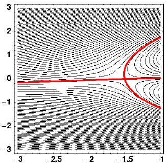
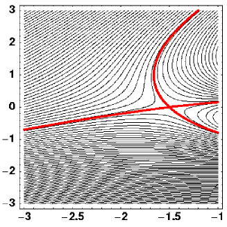
Figure 2: The heliospheric Parker spiral like magnetic field, with $10^{\circ}$ (left panel) and $40^{\circ}$ (right panel) tilting of the asymptotical magnetic field with respect to the asymptotical classical Parker (out)flow; the asymptotical Parker flow is aligned to the $x$–axis. Scale as in Fig. 1

How does this given potential field influence the strength and importance of the resistivity $R_{z}$? With the help of the asymptotical boundary conditions we get for the asymptotical electric field: $\lim_{x,y\rightarrow\infty}(R_{z}-E_{0})=-E_{0}=\frac{1}{\sqrt{\rho_{\infty}}}\,w_{\infty}B_{y\infty}$.

We calculate reconnection rates ($=$line violation rates), by using the derivative of Ohm’s law yielding

$$r=\frac{\partial}{\partial\zeta}\,\ln\frac{\partial\left(\zeta,\alpha\right)}{\partial\left(x,y\right)}$$

where the Jacobian should be regarded as a function of $\zeta$ and $\alpha$. We use Vasyliunas’ expression of line conserving flows (Vasyliunas (1972)), which shows the condition for line freezing. Line freezing is fulfilled, if $r$ vanishes everywhere. If $r$ vanishes only in the ideal region $x,y\rightarrow\infty$, line freezing is violated and reconnection is taking place.

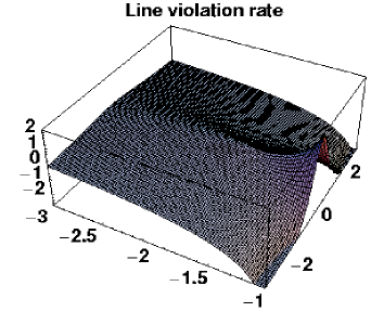
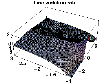
Figure 3: The line violation rate, with $10^{\circ}$ (left panel) and $40^{\circ}$ (right panel) tilting of the asymptotical magnetic field with respect to the asymptotical classical Parker (out)flow; the asymptotical Parker flow is aligned to the $x$–axis. Scale as in Fig. 1

In this case we assume, that stagnation and magnetic neutral point are identical to fix at least one point of these two pauses. With increasing angle between $\vec{w}_{\infty}$ and $\vec{B}_{\infty}$, the Parker spiral winding grows, and also the deviation of the shapes of magneto– and hydropause (see Figs. 1 and 2). Fig. 3 shows that the line violation rate is much stronger in the lower right region, where the angle $\gamma$ between the asymptotical magnetic field and the flow is larger. Here the magnetic field lines of the Parker–spiral have a higher curvature in the case of larger inclination (see right panel of Fig. 3). In Fig. 3 in front of the heliopause nose there is a bulge which shows that the reconnection rate here is larger than at other locations in the vicinity of the stagnation point.

4 Conclusions

We presented a method for calculating reconnection rates for a driven reconnection process. Further investigations need to consider non-potential fields to account for spontaneous processes including Ohmic heating. As we have shown it would be highly valuable to obtain observational knowledge of the location of magnetic neutral points and stagnation points in the heliosphere, because on the basis of that knowledge a unique solution could be given according to our prescription.

References

- Contopoulos (1996) Contopoulos, J., General axissymmetric Magnetohydrodynamic flows: Theory and solutions, Astrophys. J. 460, 185–198, 1996
- Goedbloed & Lifschitz (1997) Goedbloed, J.P., Lifschitz, A., Stationary symmetric magnetohydrodynamic flows, Phys. Plasmas 4(10), 3544–3564, 1997
- Hesse & Schindler (1988) Hesse, M., Schindler, K., A theoretical foundation of general magnetic reconnection, J. Geophys. Res., Vol. 93 No. A6, 5559–5567, 1988
- Fahr et al. (1986) Fahr, H.-J., Neutsch, W., Grzedzielski, S., Macek, W., Ratkiewicz, R., Plasma transport across the heliopause, Space Sci. Rev. 43, 329–381, 1986
- Neukirch & Priest (1996) Neukirch, T., Priest, E., Some remarks on two-dimensional incompressible stationary reconnection, Phys. Plasmas 3(8), 3188–3190, 1996
- Parker (1958) Parker, E.N., Dynamics of the interplanetary gas and magnetic fields, Astrophys. J. 128, 664–676, 1958
- Parker (1961) Parker, E.N., The stellar-wind regions, Astrophys. J. 134, 20–27, 1961
- Smith et al. (1997) Smith, E.J., Balogh, A., Burton, M.E., Forsyth, R., Lepping, R.P., Radial and azimuthal components of the heliospheric magnetic field: ULYSSES observations, Adv. Space Res. Vol. 20, 47–53, 1997
- Tsinganos (1981) Tsinganos, K.C., Magnetohydrodynamic equilibria: I. Exact solutions of the equations, Astrophys. J. 245, 764–782, 1981
- Vasyliunas (1972) Vasyliunas, V.M., Nonuniqueness of magnetic field line motion, J. Geophys. Res. 77, 6271–6274, 1972