The pulsed X-ray light curves of the isolated neutron star RBS1223

We present multi-epoch spectral and timing analysis of the isolated neutron star RBS1223. New XMM-Newton data obtained in January 2004 confirm the spin period to be twice as long as previously thought, $P_{\rm spin}=10.31$ s. The combined ROSAT, Chandra, XMM-Newton data (6 epochs) give, contrary to earlier findings, no clear indication of a spin evolution of the neutron star. The X-ray light curves are double-humped with pronounced hardness ratio variations suggesting an inhomogeneous surface temperature with two spots separated by about $\sim$160°. The sharpness of the two humps suggests a mildly relativistic star with a ratio between $R_{\rm ns}$, the neutron star radius at source, and $r_{\rm S}$, the Schwarzschild-radius, of $R_{\rm ns}/r_{\rm S}>3.5$. Assuming Planckian energy distributions as local radiation sources, light curves were synthesized which were found to be in overall qualitative agreement with observed light curves in two different energy bands. The temperature distribution used was based on the crustal field models by Geppert et al. (2004) for a central temperature of $T_{c}=10^{8}$ K and an external dipolar field of $B\sim 10^{13}$ G. This gives a mean atmospheric temperature of 55 eV. A much simpler model with two homogeneous spots with $T_{\infty}=92$ eV, and 84 eV, and a cold rest star, $T_{\rm star,\infty}<45$ eV, invisible at X-ray wavelengths, was found to be similarly successful. The new temperature determination and the new $\dot{P}_{\rm spin}$ suggest that the star is older than previously thought, $T\simeq 10^{5\dots 6}$ yrs. The model-dependent distance to RBS1223 is estimated between 76 pc and 380 pc (for $R_{\rm ns}=12$ km).

1 Introduction

RBS1223 belongs to the small elusive group of X-ray dim isolated neutron stars (XDINs) discovered in the ROSAT all-sky survey (RASS). The currently known seven systems share the properties: soft, blackbody-like X-ray spectrum, no radio emission, no association with a supernova remnant (for a review see Haberl 2004). Five objects are X-ray pulsars with spin periods in the range 3.45 to 11.37 s. The spectra of all those stars were fitted originally with pure Planckian spectra. While the spectrum of the brightest and best-studied, RX J1856.4–3754, is still compatible with a pure black-body model (Burwitz et al. 2003), recent XMM-Newton observations of RXJ0420.0-5022, RXJ0720.4-3125, RXJ1605.3+3249 (= RBS1556) and RBS1223 (= 1RXS J13048.6+212708), however, reveal significant deviations from the Planckian shape of the X-ray spectrum. These were tentatively identified with proton cyclotron absorption lines in fields of a few times $10^{13}$ G (Haberl et al. 2003, 2004, van. Kerkwijk et al. 2004). The nature of these XDINs is not clear. Their measured spin periods and moderate spin-down rates are suggestive of middle-aged neutron stars on their cooling tracks, their high surface temperatures seem to favour younger ages. The origin of their X-ray emission and their atmospheric composition is still under debate.

RBS1223 was discovered in the course of an optical identification program of the more than 2000 RASS X-ray sources at high galactic latitude with count rate CR $>0.2$ s^-1 (Schwope et al. 2000). The RASS error circle of source #1223 in this catalogue was without obvious optical counterpart at the DSS limit. Subsequent ROSAT HRI observations gave an improved X-ray position. Deep Keck imaging, $R_{\rm lim}\sim 26^{m}$, remained without optical counterpart, suggesting a high ratio $f_{\rm X}/f_{\rm opt}>10^{4}$, which excluded anything else than a neutron star as the X-ray source (Schwope et al. 1999, paper 1). Follow-up Chandra observations revealed a periodically modulated X-ray signal with an oscillation period of about 5.16 s (Hambaryan et al. 2002, paper 2). Retrospectively, we also found those oscillations in the HRI data. The derived spin-down rate of the neutron star of $\dot{P}\sim 1\times 10^{-11}$ s s^-1 implied an ultra-high magnetic field, $B_{\rm dip}>10^{14}$ G, and a characteristic age of around $10^{4}$ years, if interpreted as due to magnetic dipole braking. The decay of the field would also provide an explanation for the X-ray luminosity of the source. However, at the implied young age the source would not have been able to travel far away from its birth place. The non-detection of a close-by supernova remnant at radio wavelength or in X-rays is then at least puzzling.

We have obtained XMM-Newton observations at a first epoch in 2001 (satellite revolution rev 377) with all three EPIC cameras and both RGS’. A timing and spectral analysis of these data together with a second epoch observation was published by Haberl et al. (2003, paper 3). The much better photon statistics showed a double-humped X-ray light curve and a spin period of twice the previously reported value, $P_{\rm spin}=10.31$ s. Simple blackbody models did not fit the mean X-ray spectra at both epochs. A much better representation of the observational data was achieved after including a Gaussian-shaped absorption line superposed on a black-body spectrum. Under the assumption that the observed line is caused by a proton cyclotron line, the observed position indicates a field strength of $2-6\times 10^{13}$ G. This value would still imply a detectable spin-down rate although much smaller than derived in paper 2. If the line would be an electron cyclotron line, the implied field strength would be of order $\sim 10^{11}$ G. One would not expect to be able to detect any spin variation caused by the field decay over the comparatively short period of time that this object is observed now (1996 – 2004).

In this paper we present new data from calibration observations of RBS1223 obtained with XMM-Newton in January 2004 and GO time data obtained with the Chandra LETG on March 30, 2004. We combine all available data sets in order to update the spin history of the object. We describe a model which mimics the pulsed X-ray light curves of RBS1223. It allows to determine the sizes and temperatures of the spots on the neutron stars surface and gives also a distance estimate.

2 Observations and analysis

XMM-Newton observed RBS1223 meanwhile on three occasions. At the first epoch on Dec. 31, 2001 (XMM-Newton revolution (= rev) 377), RBS1223 was observed as a GO-target, for the following two epochs on Jan 1., 2003 (rev 561) and Dec. 30, 2003 (rev 743), it was observed as a calibration target by the XMM-Newton SOC. The first two observations were described already in paper 3, the observation in rev. 743 is almost a carbon copy of that in rev. 561, although with somewhat longer exposure time (32 ksec instead of 28  ksec). For details of the data reduction see paper 3. For the purpose of the present paper we have re-done the basic data reduction steps with the most recent version of the SAS (v6.0.0) commonly applied to all XMM-Newton data sets. A Chandra LETG observation was performed on March 30, 2004 for a total exposure of 91 ks. For the purpose of the present paper we make use of the photon arrival times of 82 ks low-background time. The spectral distribution of the photons will be investigated and published separately (Haberl et al. , in preparation).

Table 1: Spin period of RBS1223 at given epoch with given instrument. All periods listed are newly derived values.

Epoch MJD	Period	Instrument
(days)	(sec)
50824.21390	$10.31227_{-0.00011}^{+0.00012}$	Rosat HRI
51719.51835	$10.31307_{-0.00048}^{+0.00060}$	Chandra ACIS-S
52274.25598	$10.31253_{-0.00029}^{+0.00030}$	XMM PN AO1
52640.43264	$10.31250_{-0.00020}^{+0.00020}$	XMM PN CAL1
53003.46683	$10.31258_{-0.00018}^{+0.00018}$	XMM PN CAL2
53095.33034	$10.31250_{-0.00012}^{+0.00004}$	Chandra LETGS

Figure 1: The period history of RBS1223 based on X-ray observations at six epochs. The straight line represents a weighted linear fit to all data.

3 Revised period and updated spin history of RBS1223

In order to determine most likely spin periods at the different epochs we re-analysed all available data sets of RBS1223 obtained with ROSAT, Chandra and XMM-Newton using the most recent calibration files and software updates. We concentrated the period search on an interval around the value identified as the most likely spin period in Paper 3 at 10.31 s. The algorithm used was described already in Paper 2. In short, to evaluate the most probable frequency and its uncertainty in a rigorous way, we analyzed these data with the method of Gregory & Loredo (1992) based on the Bayesian formalism. This approach is free of any assumption about the pulse shape and results in an accurate parameter estimation using the probability distribution function of frequencies. The most recent data obtained with XMM-Newton confirm the 10.31 periodicity as the true spin period. This identification rests on the phase-folded light and hardness ratio curves which display a double-humped structure with unequal count rate and spectral hardness (see Fig. 2).

We re-analysed the ROSAT and the Chandra AO1 observations and found evidence for periodic variability in the interval between 10.3110 s and 10.3116 s also in those datasets, although with lower significance than at the 5.16 s periodicity. The probability that we have a periodic signal in the mentioned time interval based on the ROSAT data is 23%. For all other cases the probability is almost 100%. The measured spin periods as derived for the six epochs between June 1997 and March 2004 are listed in Tab. 1 and displayed in Fig. 1. The values given there are the most likely periods (highest peaks in the odds’ ratio periodogram), while the errors given are $1\sigma$ uncertainties (68% confidence region, ”posterior bubble”; see Gregory & Loredo 1992 and Paper 2). Weighted linear fits to all data in Tab. 1 were performed using different weighting schemes. We used either pure statistical errors taking into account the larger of the two values listed in the table, or gave weights to individual data points according to the time resolution element of the observation, the number of detected photons or the probability of detection of the periodic signal via the odds ratio. Using statistical weights only, $\dot{P}=(8.8\pm 0.4)\times 10^{-13}$ s s^-1 is derived. If weights according to the observed number of photons and the significance of detection are given in addition, the resulting $\dot{P}=(4.0\pm 0.4)\times 10^{-13}$ s s^-1 (fit shown in Fig. 1). Both fits indicate a small spin-down of the star. The evidence for a true spin-down, however, is rather weak. It rests mainly on the ROSAT HRI observation in June 1997, were only 521 photons were collected. When the first data point from Tab. 1 is omitted, a weigthed fit to the remaining data indicates even a spin-up of the neutron star, $\dot{P}=(-3.4\pm 0.4)\times 10^{-13}$ s s^-1. We conclude, that the presently available data are insufficient to determine the spin history unequivocally. This is due to the fact that the period determination for each observation has insufficient accuracy to connect subsequent observations without cycle count alias. However, our original value for the spin-down of RBS1223 is clearly ruled out.

Figure 2: Phase-averaged light curve and phase-resolved spectroscopy of the XMM-Newton observations of RBS1223 performed in revs. 561 and 743, respectively. The light curve in the top panel encompasses the spectral band 0.12 – 1.2 keV. Vertical lines indicate the boundaries of data groups for subsequent spectral analysis. In the panels below are shown the best-fit blackbody temperature, the centre, the width, the integrated flux and the equivalent widths of the Gaussian absorption line, respectively. All these parameters were determined by unconstrained fits (indicated by filled circles), by fits with fixed Gaussian line position (open triangles), and by fits with fixed Gaussian line width (open circles).

4 Phase-resolved X-ray spectroscopy

With the sufficiently large number of photons collected by XMM-Newton spinphase-resolved low-resolution X-ray spectroscopy is possible after epoch-folding and phase-averaging of the original data. Here and in the following section we use the EPIC-pn data of the two calibration observations (CALs) of RBS1223 only (revs. 561 and 743) in order to eliminate remaining calibration uncertainties between the redistribution matrices of the two CAL and the GO observations. The two CAL observations were performed in normal full frame mode with a frametime of 73 ms.

The background-corrected mean countrate detected in the pn was $2.896\pm 0.012$ s^-1 and $2.929\pm 0.012$ s^-1 for the CALs, respectively. We could not detect any long-term photometric variation among the observations with XMM-Newton. In paper 3 we have already shown that the Chandra data from AO1 are compatible with the XMM-Newton AO1 data, i.e. long-term changes of the X-ray brightness between 2000 and 2004 are insignificant.

Using the 72151 and 69435 photons detected in the two CALs we created phase-folded X-ray light curves for the two epochs. We then determined a relative phase-shift by correlating the two light curves and finally created one common phase-averaged light curve for both CALs with 100 phase bins in the energy range 0.12 – 1.2  keV. The result is shown in Fig. 2, top panel.

For our spectral analysis we defined eight phase intervals indicated by vertical lines in Fig. 2: the centres of the main and secondary pulses; the centres of the main and secondary minima; the rise and the fall to the main and secondary pulses, respectively. We adopted the same spectral model as in Paper 3, i.e. we used a blackbody plus Gaussian absorption line absorbed by the same amount of interstellar matter (represented by the column density $N_{\rm H}$). The spectral analysis was performed within XSPEC (version 11.3). Three different flavours of our adopted model were tried, the first with unconstrained parameters, a second with the centre of the Gaussian absorption line kept fix and a third with the width of the line kept fix.

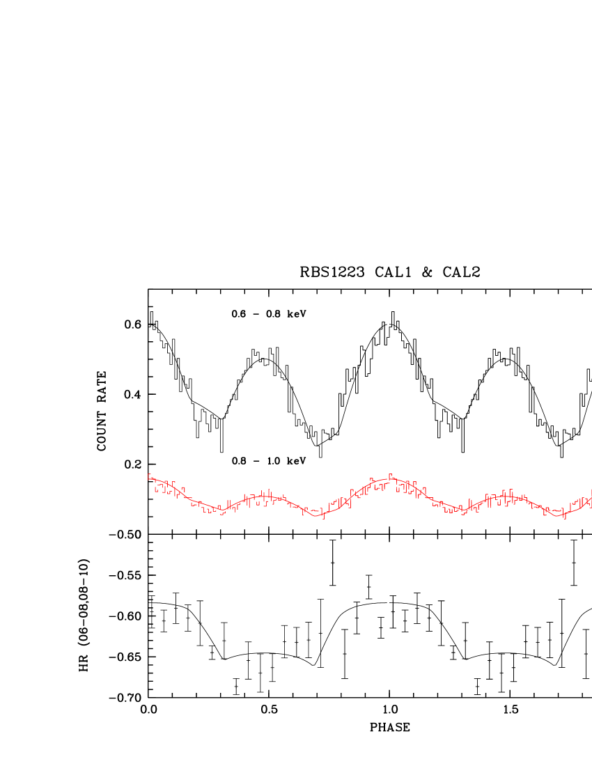
Figure 3: Soft X-ray light curves of RBS1223 in energy bands 0.6 – 0.8 keV, and 0.8 – 1.0 keV (upper panel) and corresponding hardness ratio (lower panel). The solid lines are predicted light curves based on the two spot model as described in the text.

Visual inspection of the $(O-C)$ residuals as well as an $F$-test revealed, that the observed spectrum at any given phase cannot be fitted with just one spectral (black-body) component. The inclusion of the Gaussian absorption line resulted in a satisfactory fit to all 8 spectra. The temperature drops from about 90 eV in the first hump to about 82 eV in the second hump, somewhat dependent on the chosen model. The spectral parameters are depicted in the bottom panels of Fig. 2. We found indication for a small change of the line width, being broadest in the light curve humps. Similarly, the absolute flux and the equivalent width of the Gaussian absorption line is likely to be highest in the humps. Our search for a variation of the line centre remained inconclusive.

5 Light curve analysis

The X-ray light curves of RBS1223 have a markedly double-humped shape with pronounced hardness ratio, i.e. spectral variations. The maxima and minima have unequal height. The maxima are separated by 0.47, the minima by 0.43 phase units, respectively. The occurrence of such X-ray oscillations is related to the presence of a magnetic field. Shibanov et al. (1992), Zavlin et al. (1995) and Zavlin & Pavlov (2002) have shown that the simple presence of a sufficiently strong magnetic field causes anisotropic radiation. The observed pronounced spectral variations clearly show a temperature inhomogeneity.

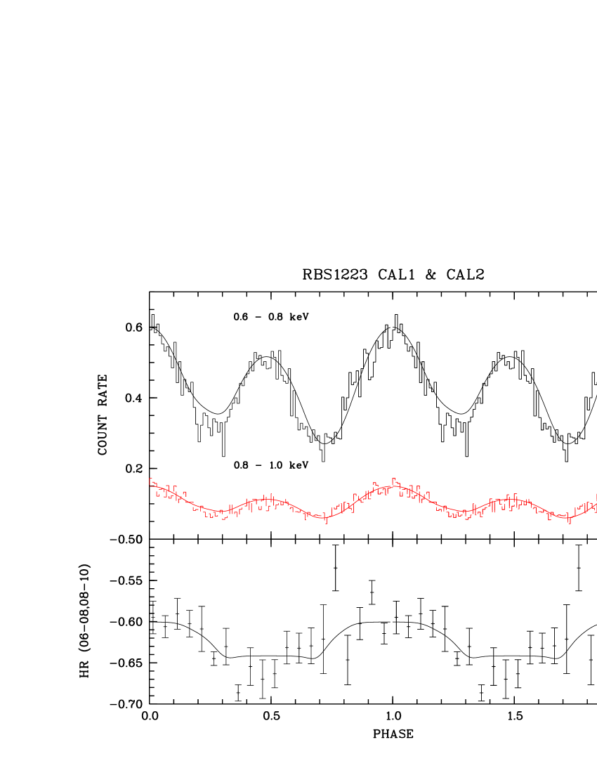
Figure 4: Observed data as in Fig. 3, the model light and hardness ratio curves are based on crustal field temperature profiles according to Geppert et al. (2004). Model parameters are described in the text.

We regard temperature inhomogeneities as the main source of the observed variations. Here we make an attempt to model the light curves assuming an inhomogenous temperature distribution over the surface of the neutron star. This is a first-order approximation, a full model would have taken into account anisotropic radiation according to the local magnetic field in a surface element. Those models are not yet available for arbitrary angles between the surface normal and the orientation of the field. As a further complication the numbers of degrees of freedom of the models would be raised by an order of magnitude. Without a proper normalization scheme and perhaps even much better data in terms of spectral and time resolution it would be very difficult to discern different models. For the time being we think that the simple approach we are following in this paper is justified by the data.

The surface of the star is tiled into small areas using constant steps in latitude and longitude. A temperature is assigned to each of the surface elements. In model ’A’ two spots of circular shape were located at certain positions, in model ’B’ a temperature distribution according to the recent crustal field models by Geppert et al. (2004) is assumed. We assume black-body radiation from each of the elements for the assumed temperature. The modeled photon spectrum is folded through the response of the XMM-Newton EPIC-pn camera. The predicted count-rate at any given time (phase) is the summed rate of all visible tiles at that phase, with an appropriate fore-shortening factor for each of the tiles. A similar approach was used by Page (1995) who gives a full description of the details.

The number of visible tiles at any given time depends on the inclination $i$ of the observer (angle between the rotation axis and the line of sight at infinity), the angle between the magnetic axis and the rotation axis $\vartheta$, and the compactness of the neutron star, parameterized by the ratio $r_{\rm gr}=R_{\rm ns}/r_{\rm S}$ ($R_{\rm ns}$: radius of the neutron star (rest frame), $r_{\rm S}$: Schwarzschild-radius). The radius and temperature in the observers frame at infinity are related to the quantities in the star’s rest frame by $R_{\infty}=R_{\rm ns}(1+z)$, $T_{\infty}=T_{\rm eff}/(1+z)$, $(1+z)^{-1}=\sqrt{1-1/r_{\rm gr}}$ ($z$: gravitational redshift).

The relevant parameters for modelling the light curves are then the radius and temperature distribution of the star, the compactness, the distance, the geometry, and the column density $N_{\rm H}$ of the interstellar absorption. Due to the unknown physical nature of the absorption feature at 0.3 keV, we restricted our light-curve analysis to the spectral regime above 0.6  keV, which is mainly unaffected by this feature. Throughout the analysis we fixed $N_{\rm H}$ at the value derived in the previous section, $N_{\rm H}=4.8\times 10^{20}$ cm^-2. We perform our analysis in two energy bands, $B_{1}=0.6-0.8$ keV, $B_{2}=0.8-1.0$ keV; the corresponding hardness ratio is defined in the usual manner as $HR=(CR_{2}-CR_{1})/(CR_{1}+CR_{2})$, $CR_{1,2}$ being the count rates in the two defined energy bands. For any given $N_{\rm H}$ the hardness ratio is a direct measure of the blackbody temperature.

Beloborodov (2002) has studied the bending of light in the vicinity of compact objects. He derived a simple approximate relation between the local angle of photon emission, $\alpha$, and the escape direction, $\psi$: $1-\cos\alpha=(1-\cos\psi)(1-r_{\rm gr})$. It has a maximum deviation of 3% for $r_{\rm gr}=3$ with respect to the exact theory (Pechenick et al. 1983). The visible fraction of the star is derived from this relation by setting $\alpha=90\degr$ (see his Fig. 1). We use this approximation in order to determine the visible fraction of the neutron star’s surface as well as the foreshortening angle of individual surface elements.

Beloborodov also studied the possible types of light curves as a function of $i$ and $\vartheta$ if two spots are located diametrically opposite on the magnetic axis. His class III is describing the current situation of RBS1223 with the two spots rotating subsequently into view. This type of light curve is observed, when $\cos(i+\vartheta)<-r_{\rm S}/(R-r_{\rm S})$, i.e. when both angles $i$ and $\vartheta$ are sufficiently large. Although in principle a large range of combinations between $i$ and $\vartheta$ produces light curves of type III, the pulsed fraction is maximized for $i=\vartheta$, which we assume in the following.

We ran a number of simulations exploring the parameter space searching for an optimum solution by a fit-per-eye. Our finally accepted light-curve solution giving best overall qualitative agreement with the observed data is shown in Fig. 3. The parameters in our model ’A’ are constrained by the following observed features.

The pulsed fraction of the light curve is rather high, $p=(CR_{\rm max}-CR_{\rm min})/CR_{\rm max}\sim 52\%$ in the soft band $B_{1}$, which constrains the compactness of the star. For $r_{\rm gr}<3.5$ a too large fraction of the star becomes visible at any given time. This damps the amplitude of the variation below the observed value. In the following we assume $r_{\rm gr}=4$. This retrospectively justifies the use of Beloborodov’s approximative formula for the description of light bending, which is applicable only to not too compact objects.

The observed large pulsed fraction also requires a high inclination $i$ (and a high $\vartheta$ for our assumed geometry with $i=\vartheta$), $i>75\degr$, although one can trade to some extent a higher compactness parameter against a lower inclination and vice versa. The model light curve shown in Fig. 3 was computed for $i=\vartheta=80\degr$ and $r_{\rm gr}=4$.

The temperature of the main spot is fixed by the observed hardness ratio in the main hump of the light curve to $T_{1,\infty}=92$ eV. The width of the main hump constrains the maximum extent of the spot, the full opening angle of the main spot is of order $2\theta_{1}\sim 8\degr$.

The location of the second spot is constrained by the observed separation between the maxima and minima of the light curve. We locate the second spot at an offset angle of $\kappa=20\degr$ with respect to the magnetic axis and at an azimuth of about $20\degr$. The offset $\kappa$ is not very well constrained by the observations. It could become larger if the spot is located closer to the meridian through the rotation and the magnetic axis. Under extreme circumstances, $\kappa$ can become as large as $50\degr$, although the fit then clearly deteriorates, hence we estimate the minimum separation between the two spots to be $\sim$130°.

The temperature of the second spot is determined by the observed spectral hardness in the pulse maximum, $T_{2,\infty}=84$ eV. The width of the second pulse and the relative brightness of the second with respect to the first spot then suggest a full opening angle somewhat larger as for the main pulse, $2\theta_{2}\sim 10\degr$.

The contribution of the remaining surface in this model is negligible, the light and hardness ratio curves are almost completely determined by emission from the two spots. This contrains the atmospheric temperature to $T_{\rm star,\infty}<42$ eV. The maximum possible $T_{\rm star,\infty}$ is 50 eV. This limit is derived under the extreme assumption $r_{\rm gr}\gg 1$. In this non-relativistic limit the two spots rotate alternating into view and the emission between the two humps is entirely due to photospheric emission.

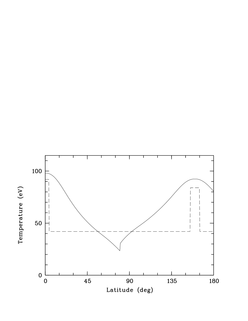
Figure 5: Temperature distribution as a function of magnetic colatitude for models ’A’ (dashed line) and ’B’ (solid line), respectively. The temperatures are given in eV. The stellar temperature of model ’A’ is an upper limit as derived from the light curve modeling. This limit violates the constraint from the broad-band spectral energy distribution as sown in Fig. 6 which requires a remaining star of almost zero temperature.

Finally the modeled light curve is normalized to the observed curve by a $(R_{\infty}/D)^{2}$ factor. For our model ’A’ we derive a distance $D$ of only 76 pc for an assumed $R_{\rm ns}=12$ km star ($R_{\infty}=13.8$ km for $r_{\rm gr}=4$). Our best-fit model curve for model ’A’ is shown in Fig. 3. The corresponding temperature variation along stellar latitude is shown in Fig. 5 for an assumed atmospheric temperature of 42 eV. It is emphasized again that the fit of the light curve is based on an adaption per eye and not due to a formal least-squares fit.

Having set the main scenery with our ad hoc two-spot model, we proceed by comparing the observed light curves with the predictions for the temperature distribution in a magnetized neutron star crust. Such distributions became recently available (Geppert et al. 2004) and these authors kindly provided tabulated data. Geppert et al. calculated the temperature distributions in the atmosphere for the ’core’ and ’crustal’ field scenario. They solve the equation of heat transport through the star’s atmosphere in the presence of a given dipolar field, the main parameters which determine the temperature distribution being the (isothermal) core temperature $T_{c}$ and the dipolar field strength. The $T$-distribution of their crustal models for sufficiently high magnetic field strength resembles the situation studied here with two warm spots. Moreover, the maximum temperature of their $T_{c}=10^{8}$ K model is of the same order as the spot temperature in RBS1223. The ’core’ field scenario a la Greenstein & Hartke (1983) always produces a too flat $T$-distribution and is not further considered here.

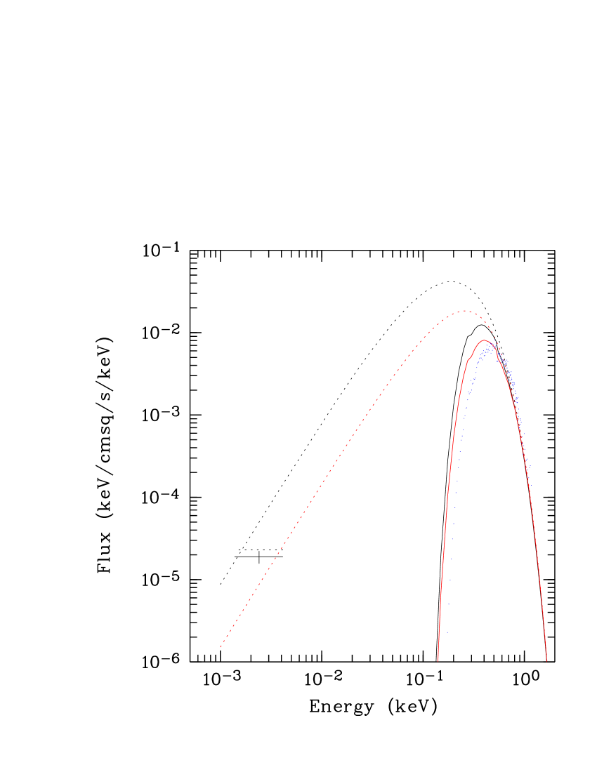
Figure 6: Broad-band spectral energy distribution of RBS1223. Shown with solid lines are the absorbed blackbody spectra which agree the XMM-Newton EPIC pn data at phase of the main hump, with dotted lines the unabsorbed extrapolations to low energies for models A (lower red lines) and B (upper black lines), respectively. The data point at 2.4 eV represents the $m_{\rm 50CCD}=28.56\pm 0.13$ mag tentative optical counterpart (Kaplan et al. 2002a). The unfolded observed X-ray spectrum at phase of the main hump is shown with small blue symbols.

In order to compute synthetic lightcurves we used the published $T$-distributions from Geppert et al. (plus one unpublished distribution for $T_{c}=10^{8}$ K and $B=10^{14}$ G). We parameterized the maximum temperature as a function of given $T_{c}$ and $B$ using a bi-polynomial interpolation. This allows an easy scaling of a chosen $T$-profile to the observed maximum temperature. For light curve synthesis we used the same viewing and magnetic geometry and the same compactness parameter $r_{\rm gr}$ as above for our initial toy model ’A’. The star was divided into two half-spheres so that different $T$-distributions could be applied to the two halfs. This somewhat artificial approach was necessary in order to simulate the two observed unequal spots. The two half spheres were slightly inclined with respect to each other, in order to match the observed phases of the light curve maxima and minima.

The normalized $T$-profiles chosen for the main and secondary humps correspond to $T_{c}=10^{8}$ K, $\log B\mathrm{(G)}=14$, and $T_{c}=10^{8}$ K, $\log B\mathrm{(G)}=13.7$, respectively.

A maximum temperature of 98 eV in the main spot was achieved assuming a core temperature $T_{c}=10^{8.04}$ K and a dipolar field of $\log B\mathrm{(G)}=13.0$. In order to model the observed lower temperature in the second spot, we had to assume a slightly lower temperature $T_{c}=10^{8.02}$ K and a slightly lower field strength $\log B=12.5$ G as well. This parameter combination then yields the maximum temperature in the spot of 91 eV. The fit based on the described combination of parameters is shown in Fig. 4. As above, we used a radius of the neutron star $R_{\infty}=13.8$ km. The implied distance derived for the crustal field model is then 380 pc. This value is clearly much larger than that of the simple two-spot model since a much larger fraction of the star’s surface contributes to the observed light.

Hence, the crustal field temperature profiles seem to be equally suited to reflect the observed light curves of RBS1223. We note, however, that our approach is not selfconsistent, since the maximum spot temperature and the $T$-profiles were adapted in separate steps. In addition, the simulated $T$-profiles were computed for a more compact star, $R_{\rm ns}=10$ km, $M=1.4$ M_⊙, than assumed here. This might explain the inconsistency between the values of the parameters $T_{c},B$ used to determine the maximum temperature in the spots and the corresponding $T$-profile used by us. The temperature distribution which matches the observed narrow pulses is steeper than implied by the maximum temperature in the spot.

6 Results and discussion

We have presented a multi-mission timing analysis of the isolated neutron star RBS1223. New observations with XMM-Newton gave further support for a revised spin period at 10.31 s. The spin history could not yet be uncovered without ambiguity, the previously derived significant spin-down however seems to be ruled out by the series of XMM-Newton observations. This finding most probably rules out a magnetic field strength in excess of $10^{14}$ G. A field estimate based on the energy loss of a rotating vacuum dipole magnetosphere $B\sin{\vartheta}\simeq 10^{12}\sqrt{P\dot{P}_{\rm-13}}$ reveals with $P=10$ s, $\dot{P}=4\times 10^{-13}$ s s^-1 and $\vartheta=80\degr$ a field strength of $B\simeq 6\times 10^{13}$ G. However, the present data even do not reveal clearly a spin-down of the star. The omission of the least significant spin value based on the 1996 ROSAT observation is indicative even of a spin-up of the star. The unequivocal determination of the spin history of RBS1223 without cycle count alias is possible by a dedicated campaign with XMM-Newton which is already granted.

The long-term observations and the analysis presented here shed some new light on the likely nature of RBS1223. We mention firstly, that there is no long-term change of the brightness of RBS1223. This makes Bondi-Hoyle accretion as powering mechanism of the X-ray source unlikely.

The spin-phase averaged light curve is double-humped with two humps of different count rate and spectral hardness. The humps are separated by about 0.47 phase units, the minima by about 0.43 phase units, which indicates a slight asymmetry of the shape of the individual humps. The double-humped light curves is indicative for the presence of a moderately strong field which is not axisymmetric. A displaced dipole or contribution(s) from higher multipoles are likely causes for the asymmetry.

We performed a phase-resolved X-ray spectral analysis of the two calibration observations in 2003 and 2004. A successful fit to the spectra at all phases was achieved by the combined black-body plus Gaussian absorption line model. There is a clear temperature variation over the spin cycle, also the line centre, the line flux and the line equivalent width show cyclic changes. The combined new data do not allow to constrain the nature of the Gaussian further, we still regard the cyclotron absorption line scenario as possible.

The observed variations of the spectral parameters are, however, different from those observed in RX J0720.4–3125 (henceforth RX0720) by Haberl et al. (2004). In RX0720 the temperature variations are much smaller, $\Delta T\simeq 2.5$ eV only. The equivalent widths of the putative cyclotron absorption lines change in both systems by about 50%, the equivalent width in RBS1223 is a factor 2–3 larger than in RX0720. While RX0720 shows a trend that larger equivalent width corresponds with lower blackbody temperature there is no such trend in RBS1223.

The double-humped light curve is suggestive of a spotted atmosphere of the star with two spots separated by about 160 degrees. We presented two similarly successful fits to the X-ray light curves in two energy bands. The chosen energy bands for our experiment, 0.6–0.8, and 0.8–1.0 keV respectively, are thought to be unaffected by the absorption feature so that simple blackbody spectra could be used for light curve synthesis. Taking the view of the simple model ’A’, the star is described by two visible spots of size 8° and 10° and a, for X-ray eyes, invisible remaining surface. The atmospheric temperature of less than 42 eV (500000 K) leads to a revised age estimate of about $10^{5\dots 6}$ years (derived from cooling curves of Lattimer & Prakash 2004). This revision solves the problem between the estimated young age and the non-detection of an associated supernova remnant (paper 2).

In Fig. 6 the broad-band spectral energy distribution of RBS1223 is shown. The best-fit X-ray spectra for the main hump based on our models ’A’ and ’B’ (mean spectra of the visible hemispheres) are extrapolated to the optical. The data point in the optical wavelength range at 2.4 eV stretching from 3000 to 9000 Å represents the brightness of the $m_{\rm 50CCD}=28.56\pm 0.13$ mag tentative optical counterpart dicovered by Kaplan et al. (2002a). The extrapolation indicates that the brightness of the likely optical counterpart is compatible with our models. Any further low temperature component would raise the predicted flux at optical wavelength over the observed value. However, the blackbody models which were adjusted in the energy bands 0.6-0.8, and 0.8-1.0 keV, respectively, already overpredict the X-ray flux below 0.5 keV were the Gaussian absorption line is observed. The extrapolation into the optical may therefore be done only with caution.

The predicted distance to RBS1223 based on model ’A’ is uncomfortably short, 76 pc, i.e. nearer than the much brighter prototypical system RX  J1856.5-3754 ($D_{\rm RXJ1856}=140\pm 40$ pc, Kaplan et al. 2002b). The short distance is due to the simplicity of the temperature structure and geometry. Any temperature profile with a more gradual variation of the temperature and corresponding larger parts of the stellar surface contributing to the observed light will requires larger distances to the star. Model ’A’ was used as a toy model in order to constrain the geometry and the compactness, but it lacks a physical interpretation.

The physical interpretation is possible with our model ’B’, based on the crustal field model by Geppert et al. (2004). This reflects the data equally well. In this model the spots are more extended, i.e. larger parts of the atmosphere contribute to the observed radiation. The estimated distance is consequently much larger, $D\sim 380$ pc (all distance estimates were made for a 1 M_⊙ star with radius $R_{\rm ns}=12$ km and $R_{\rm ns}/r_{\rm S}=4$). However the parameter set based on model ’B’ is not completely consistent. The average temperature of the atmosphere is higher than for model ’A’, 55 eV, but still clearly lower than previously assumed so that the age problem is solved also with model ’B’.

Given the very restricting assumptions of our spectral model, pure black-body emission with a simple foreshortening law, the results of the study presented here can be regarded only as a first step towards a full model of the star. As worked out by Pavlov et al. (1996) and re-addressed by Zavlin & Pavlov (2002) atmosphere model fits give temperatures $T_{\rm atm}$ significantly lower than the blackbody temperature $T_{\rm bb}$ (dependent on the chemical composition). Light-element models, however, which would show the most drastic effect are likely ruled out, since they predict much higher fluxes in the RJ-part of the spectrum. They also would predict much shorter distances compared to bb-models, which doesn’t seem very likely. Fe-models, on the other hand, do not show dramatic differences as far as $T_{\rm eff}$ and the predicted distance are concerned. Since they produce less optical flux they seem to be much better suited to fit the spectral energy distribution than bb- or light element models. Another point of uncertainty is the type of the assumed foreshortening. Zavlin & Pavlov (2002) computed the angular characteristic of specific intensities with an assumed field perpendicular to the surface which shows strongly peaked emission normal to the surface. If applicable to the case of RBS1223 this would clearly affect the spin-phased light curves. Future light curve models would strongly benefit from the availability of a dense grid of models for different temperature, magnetic field strength, chemical composition and angle between the local magnetic field and the surface normal. Based on such grid, light curve modeling would be possible via a regularisation scheme in the multidimensional parameter space.

In sum, the revised value for $\dot{P}$ together with the revised value for the mean atmospheric temperature suggest a nature of RBS1223 as a medium-aged neutron star ($10^{5\dots 6}$ yrs) on its cooling track. The nature of the Gaussian is not understood, it could be a cyclotron absorption line in a field of a few $10^{13}$ G, still compatible with the (uncertain) spin-down. The present distant estimates make the star similarly close as the prototype RXJ1856, which has a large observed proper motion and a measured parallax. Although very much fainter, $m_{\rm 50CCD}=28\aas@@fstack{m}6$ (Kaplan et al. 2002a), a similar measurement for RBS1223 seems to be feasible and rewarding in order to further constrain the likely distance, radius and thus nature of this star.

- (1) Beloborodov, A.M. 2002, ApJL 566, 566
- (2) Burwitz, V., Haberl, F., Neuhäuser, R., Predehl, P., Trümper, J., Zavlin, V.E., 2003, A&A 399, 110
- (3) Geppert, U.R.M.E., Küker, M., Page, D., 2004, A&A 426,267
- (4) Greenstein, G., Hartke, G.J., 1983, ApJ 271, 283
- (5) Gregory, P., Loredo, T., 1992, ApJ 398, 146
- (6) Haberl, F. 2004, Adv. Sp. Res. 33, 638
- (7) Haberl, F., Schwope, A.D., Hambaryan, V., Hasinger, G., Motch, C., 2003, A&A 403, L19 (paper 3)
- (8) Haberl, F., Zavlin, V.E., Trümper, J., Burwitz, V., 2004, A&A 419, 1077
- (9) Hambaryan, V., Hasinger, G., Schwope, A.D., Schulz, N.S., 2002, A&A 381, 98 (paper 2)
- (10) Kaplan, D.L., Kulkarni, S.R., van Kerkwijk, M.H., 2002a, ApJ 579, L29
- (11) Kaplan, D.L., van Kerkwijk, M.H., Anderson, J., 2002b, ApJ 571, 447
- (12) Lattimer, J.M., Prakash, M., 2004, Science 304, 536
- (13) Page, D., 1995, ApJ 442, 273
- (14) Pavlov, G.G., Zavlin, V.E., Trümper, J., Neuhäuser, R., 1996, ApJL 472, 33
- (15) Pechenick K.R., Ftaclas, C., Cohen, J.M. 1983, ApJ 274, 846
- (16) Schwope, A.D., Hasinger, G., Schwarz, R., Haberl, F.W., Schmidt, M., 1999, A&A 341, L51 (paper 1)
- (17) Schwope, A.D., Hasinger, G., Lehmann, I., et al., 2000, AN 321, 1
- (18) Shibanov, Yu.A., Zavlin, V.E., Pavlov, G.G., Ventura, J., 1992, A&A 266, 313
- (19) van Kerkwijk, M.H., Kaplan, D. L., Durant, M., Kulkarni, S.R., Paerels, F., 2004, ApJ 608, 432
- (20) Zavlin, V.E., Pavlov, G.G., Shibanov, Yu.A., Ventura, J., 1995, A&A 297, 441
- (21) Zavlin, V.,E., Pavlov, G.G., 2002, MPE report 278, 263