Sub-milliarcsecond Imaging of Quasars and Active Galactic Nuclei
IV. Fine Scale Structure

Abstract

We have examined the compact structure in 250 flat-spectrum extragalactic radio sources using interferometric fringe visibilities obtained with the VLBA at 15 GHz. With projected baselines out to 440 million wavelengths, we are able to investigate source structure on typical angular scales as small as 0.05 mas. This scale is similar to the resolution of VSOP space VLBI data obtained on longer baselines at a lower frequency and with somewhat poorer accuracy. For 171 sources in our sample, more than half of the total flux density seen by the VLBA remains unresolved on the longest baselines. There are 163 sources in our list with a median correlated flux density at 15 GHz in excess of 0.5 Jy on the longest baselines; these will be useful as fringe-finders for short wavelength VLBA observations. The total flux densities recovered in the VLBA images at 15 GHz are generally close to the values measured around the same epoch at the same frequency with the RATAN–600 and UMRAO radio telescopes.

We have modeled the core of each source with an elliptical Gaussian component. For about 60% of the sources, we have at least one observation in which the core component appears unresolved (generally smaller than 0.05 mas) in one direction, usually transverse to the direction into which the jet extends. BL Lac objects are on average more compact than quasars, while active galaxies are on average less compact. Also, in an active galaxy the sub-milliarcsecond core component tends to be less dominant. Intra-Day Variable (IDV) sources typically have a more compact, more core-dominated structure on sub-milliarcsecond scales than non-IDV sources, and sources with a greater amplitude of intra-day variations tend to have a greater unresolved VLBA flux density. The objects known to be GeV gamma-ray loud appear to have a more compact VLBA structure than the other sources in our sample. This suggests that the mechanisms for the production of gamma-ray emission and for the generation of compact radio synchrotron emitting features are related.

The brightness temperature estimates and lower limits for the cores in our sample typically range between $10^{11}$ and $10^{13}$ K, but they extend up to $5\,\times\,10^{13}$ K, apparently in excess of the equipartition brightness temperature, or the inverse Compton limit for stationary synchrotron sources. The largest component speeds are observed in radio sources with high observed brightness temperatures, as would be expected from relativistic beaming. Longer baselines, which may be obtained by space VLBI observations, will be needed to resolve the most compact high brightness temperature regions in these sources.

1. Introduction

Early interferometric observations of radio source structure were typically analyzed by examining how the amplitude of the fringe visibility varied with projected interferometer spacing (e.g., Rowson 1963). Although these techniques for conventional connected interferometers were later replaced by full synthesis imaging incorporating Fourier inversion, CLEAN (e.g., Högbom 1974), and self calibration (see review by Pearson & Redhead 1984), the interpretation of the early VLBI observations, again, was based on the examination of fringe amplitudes alone (see Cohen et al. 1975). Indeed, the discovery of superluminal motion in the source 3C 279 (catalog ) (Cohen et al. 1971, Whitney et al. 1971) was based on single baseline observations of the change in spacing of the first minimum of the fringe visibility. However, after the development of phase-closure techniques, reliable full synthesis images have been produced from VLBI observations for more than 25 years. However, these tend to hide the information on the smallest scale structures, because of the convolution with the synthesized beam (e.g., Figure 1). A more thorough discussion of non-imaging VLBI data analysis is given by Pearson (1999).

The best possible angular resolution is needed to study the environment close to supermassive black holes where relativistic particles are accelerated and collimated to produce radio jets. The greatest angular resolution to date was obtained in observations of interstellar scintillations (e.g., Kedziora-Chudczer et al. 1997, Macquart et al. 2000, Kedziora-Chudczer et al. 2001, Jauncey & Macquart 2001, Rickett et al. 2001, Dennett-Thorpe & de Bruyn 2002, Kraus et al. 2003, Lovell et al. 2003). The resolution achievable with VLBI can be improved by observing at shorter wavelengths (e.g., Moellenbrock et al. 1996, Lobanov et al. 2000, Lister 2001, Greve et al. 2002) or by increasing the physical baseline lengths using Earth-to-space interferometry. The first space VLBI missions (Levy et al. 1989, Hirabayashi et al. 1998) increased the available baseline lengths by a factor of about 3. Planned space VLBI observations such as RadioAstron (Kardashev 1997), VSOP–2 (Hirabayashi et al. 2004), and ARISE (Ulvestad 2000), will extend the baselines further.

Figure 1.— Comparison of two epochs for the quasar 0906+015. Top: visibility function amplitude (i.e. correlated flux density), $S_{\mathrm{c}}$, versus projected spacing, $r_{uv}$. Bottom: naturally weighted CLEAN images. The lowest contour is plotted at the level of 0.16% and 0.13% of the peak brightness of 0.87 (epoch 1997/08/18) and 1.79 (epoch 1999/05/21) Jy/beam, respectively. Other contours are shown at increasing powers of $\sqrt{2}$. The half-power width of the synthesized beam (with natural weighting) is shown in the left lower corners. The ($u$,$v$)-coverage of the two experiments was similar. One can clearly see (and model) from the $S_{\mathrm{c}}$–$r_{uv}$ plots that an unresolved component observed at the first epoch at a level of about 0.8 Jy is heavily resolved at the second epoch, which is not clear from the corresponding CLEAN images. This component dominates the $S_{\mathrm{c}}$–$r_{uv}$ dependence.

For simple source structures, a direct study of the fringe visibilities can give a better angular resolution than an analysis of the images reconstructed from these data (e.g., Maltby & Moffet 1962). In principle, a careful deconvolution of the images should give equivalent results. However, experience has shown that when confronted with even moderately complex images, it is dangerous to attempt to increase the resolution significantly beyond that of the CLEAN restoring beam size; a procedure referred to in early radio astronomy literature as “super resolution”.

In two previous papers (Kellermann et al. 1998, hereafter Paper I, and Zensus et al. 2002, hereafter Paper II) we have described the sub-milliarcsecond scale structure of 171 active galactic nuclei, based on naturally weighted images made from observations with the VLBA (Napier et al. 1994) at 15 GHz. In addition, in Paper II we have placed more restrictive limits on the sizes of unresolved sources by direct analysis of the fringe visibilities. In a third paper (Kellermann et al. 2004, hereafter Paper III) we have reported on the observed motions in the jets of 110 of these sources during the period 1994 to 2001.

In this paper, we analyze 15 GHz VLBA observations of the central regions of 250 extragalactic radio sources. We use the visibility function data to study the most compact structures and the way they change with time. The smallest features we are able to discern from these data have an extent of about 0.02–0.06 mas. For the nearest object in our study, 1228+126 (catalog ) (M 87 (catalog ), Virgo A (catalog )), this corresponds to a linear size of $10^{16}$ cm, or several tens of Schwarzschild radii, if the mass of the central object is $3\,\times\,10^{9}$ solar masses and the distance is 17.5 Mpc. We define our sample in § 2, describe the visibility data in § 3, and the model fitting and analysis in § 4. In § 5 we discuss the results, and the conclusions are summarized in § 6.

Throughout this paper we use the following cosmological parameters: $H_{0}=70$ km s^-1 Mpc^-1, $\Omega_{\mathrm{m}}=0.3$, and $\Omega_{\Lambda}=0.7$. We adopt the convention of using the term “quasar” to describe optical counterparts brighter than absolute magnitude $-23$, and “active galaxy” for the fainter objects.

2. Sample Definition

Our analysis is based on data obtained during the period 1994–2003 as part of the VLBA 15 GHz monitoring survey of extragalactic sources (Papers I, II, and III, Lister & Homan 2005, E. Ros et al., in preparation). We have also used additional observations made in 1998 and 1999 by L. I. Gurvits et al. (in preparation) as part of a separate program to compare 15 GHz source structure measured with the VLBA to 5 GHz structure measured in the framework of the VSOP Survey Program (Hirabayashi et al. 2000, Lovell et al. 2004, Scott et al. 2004, Horiuchi et al. 2004). The program by Gurvits et al. used the same observing and data reduction procedures as the VLBA 15 GHz monitoring survey, and provides both additional sources and additional epochs.

Our dataset consists of 1204 VLBA observations of 250 different compact extragalactic radio sources. The initial calibration of the data was carried out with the NRAO $\cal{AIPS}$ package (Greisen 1988), and was followed by imaging with the DIFMAP program (Shepherd 1997), mostly with the use of an automatic script (, ). The CLEAN images as well as the visibility function data are available on our web sites.

Most of the radio sources contained in our “full sample” of 250 sources have flat radio spectra ($\alpha>-0.5$, $S_{\nu}\sim\nu^{\alpha}$), and a total flux density at 15 GHz (often originally estimated by extrapolation from lower frequency data) greater than 1.5 Jy for sources with declination $\delta>0^{\circ}$, or greater than 2 Jy for sources with $-20^{\circ}<\delta<0^{\circ}$. However, additional sources which did not meet these criteria but are of special interest were also included in the full sample.

Our full sample is useful for investigating fine scale structure in a cross-section of known extragalactic radio source classes, and for planning future (space) VLBI observations. However, in order to compare observations with the theoretical predictions of relativistic beaming models, it is also useful to have a well-defined sub-sample selected on the basis of beamed, rather than total, flux density. We have therefore formed a flux density limited complete sample which has been used as the basis of our jet monitoring program since mid 2002, called “The MOJAVE Program: Monitoring Of Jets in AGN with VLBA Experiments” (Paper III, Lister & Homan 2005). There are 133 sources in the MOJAVE sub-sample. The redshift distribution for these sources ranges up to 3.4 (quasar 0642+449 (catalog )), although most sources have redshifts less than 2.5, with a peak in the distribution near 0.8.

Table 1 summarizes the properties of each source. Columns 1 and 2 give the IAU source designation, and where appropriate, a commonly used alias; J2000.0 coordinates are in columns 3 and 4. The optical classification and redshift are shown in columns 5 and 6, respectively; these were obtained mainly from Véron-Cetty & Véron (2003), as discussed below. In column 7 we give a radio spectral classification for each source based on the RATAN–600 radio telescope observations of broad-band instantaneous spectra from 1 to 22 GHz (Kovalev et al. 1999, 2000). These spectra are available on our web site. For the few sources which were not observed at RATAN–600, we used published (non-simultaneous) radio flux densities taken from the literature. We consider a radio spectrum to be “flat” if any portion of its spectrum in the range 0.6 GHz to 22 GHz has a spectral index flatter than $-0.5$ and “steep” if the radio spectral index is steeper than $-0.5$ over this entire region. In column 8 we indicate whether or not the radio source is associated with a gamma-ray detection by EGRET (Mattox et al. 2001, Sowards-Emmerd et al. 2003, 2004). Columns 9 and 10 indicate whether or not the source is a member of the complete correlated flux density limited MOJAVE sample and the VSOP 5 GHz AGN survey source sample (Hirabayashi et al. 2000, Lovell et al. 2004, Scott et al. 2004, Horiuchi et al. 2004). Column 11 gives references to papers reporting intra-day variability (IDV) of the source total flux density.

Of the 250 sources in the full sample, there are 179 quasars, 37 BL Lacertae objects, 23 active galaxies, and 11 sources which are optically unidentified. The MOJAVE complete sample of 133 sources includes 94 quasars, 22 BL Lacertae objects, 8 active galaxies, and 9 unidentified objects. These classifications come from Véron-Cetty & Véron (2003), who defined a quasar as a star-like object, or an object with a star-like nucleus, with broad emission lines, brighter than absolute magnitude $\mathrm{M_{B}}=-23$.

Véron-Cetty & Véron (2003) provide a list of BL Lacertae objects, which historically were defined as bright galactic nuclei which are highly polarized in the optical regime, and for which no emission or absorption lines have been detected. The precise delineation between BL Lacs and OVV quasars remains controversial (Véron-Cetty & Véron 2000), since the original proposed 5 Å limit (Stickel et al. 1991) is arbitrary (Scarpa & Falomo 1997), and individual emission line equivalent widths are now known to be highly variable over time. Indeed the prototype, BL Lac itself, shows broad and narrow emission lines, as well as stellar absorption lines, in modern spectra: it no longer meets the classical definition of a BL Lac (Vermeulen et al. 1995). The detectability of narrow and broad emission lines and absorption lines is set to a very significant degree by the variable continuum level, signal-to-noise ratio (SNR), starlight contribution, and other extrinsic and time-dependent factors (see, e.g., Marcha & Browne 1995). The situation is complicated further by proposed unification schemes (Urry & Padovani 1995), which apparently led Véron-Cetty & Véron (2003) to re-classify many BL Lacs as quasars solely on the basis of their extended 5 GHz luminosity being above the FR I/II division.

Many of the objects in our sample are blazars, which are defined as the union of the original categories of BL Lacertae objects and optically violently variable (OVV) quasars. Both groups are highly polarized and variable in the optical spectral region (e.g., Angel & Stockman 1980). Since we are interested in comparing the radio properties of strong and weak-lined blazars, we retain the original BL Lac classifications for these objects and indicate these and other controversial classifications in the notes to Table 1. For our analysis, it would have been preferable to directly use optical line equivalent width data; however, high-quality, multi-epoch spectra are currently available for only a small fraction of our sample. Nevertheless, the objects originally classified as BL Lacs do, on average, have lower equivalent width spectral lines than classical quasars. This seems to be (i) partly the effect of dilution by a beamed non-thermal continuum (e.g., Wills et al. 1983), and (ii) partly because many of these objects are intrinsically different from classical quasars as shown by their diffuse radio emission which is similar to that of FR I radio galaxy (e.g., Kollgaard et al. 1992, Rector & Stocke 2001). These two effects cannot be clearly separated using only VLBI data. We show here that on average objects historically called “BL Lacs” differ statistically from classical quasars in their parsec scale radio properties. Physical interpretation depends on separating the above two effects.

3. Visibility functions

Figure 2.— Amplitude of the visibility function (i.e. correlated flux density), $S_{\mathrm{c}}$, versus projected spacing, $r_{uv}$. Each point represents a coherent average over one 4–6 min observation on an individual interferometer baseline. The error bars, which represent only the statistical errors, are often smaller than the symbol. Errors of the absolute flux density calibration are not shown here and are about 5%. For each source, the data are presented at the epoch when $S_{\mathrm{unres}}$ is maximum. The plots for all the epochs observed in the 15 GHz VLBA monitoring program until 2003/08/28 are shown in the electronic version.

Figure 3.— Continued

Figure 4.— Continued

Figure 5.— Continued

Figure 6.— Continued

Figure 7.— Continued

Figure 8.— Continued

Figure 9.— Continued

Figure 10.— Continued

Figure 11.— Continued

Figure 12.— Continued

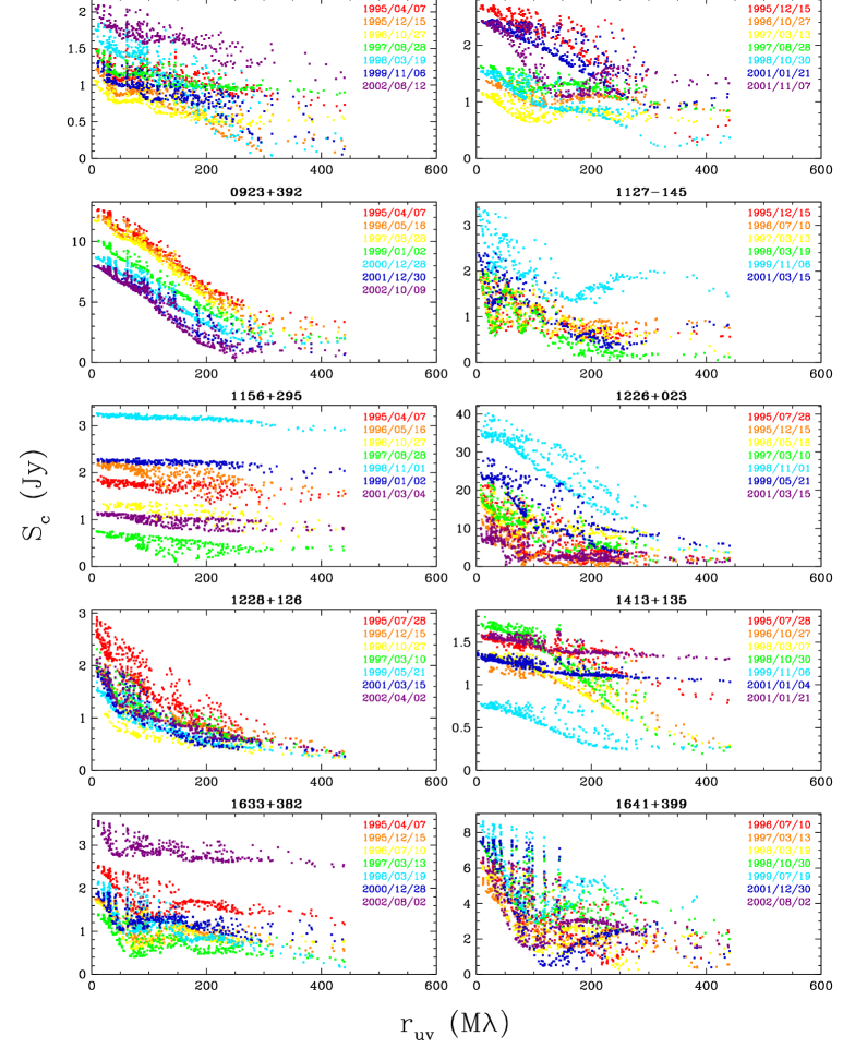
Figure 13.— Examples of the time variability of the correlated flux density versus projected spacing for ten representative sources. Different epochs are denoted by different colors in their spectrum-color order.

Our 15 GHz VLBA images, made with natural weighting of the visibility data, have a nominal resolution of 0.5 mas in the east–west direction and 0.6–1.3 mas in the north-south direction. The fringe spacing of the VSOP Survey at 5 GHz (Lovell et al. 2004, Scott et al. 2004, Horiuchi et al. 2004) is similar to that of the VLBA at 15 GHz, but the effective resolution of the VLBA is better, thanks to the relatively high SNR on the longest baselines, and to the good relative calibration of the fringe visibilities, which can be determined with self calibration using higher quality images based on many more interferometer baselines, and full hour angle coverage. Typically the dynamic range of the VLBA images (the ratio of the peak flux density to the rms noise level) is better than 1000:1 (, , Lister & Homan 2005).

Figure 2 shows the visibility function amplitudes (correlated flux density versus projected baseline length) for each source in the full sample at the epoch when the amplitude is the highest at the longest projected spacings . These plots are independent of any assumptions about the source structure, imaging artifacts, or beam smoothing; and, more directly, they can show the presence of structure on scales smaller than the synthesized beam. Also, as illustrated in Figure 13, many of these sources are variable. Changes with time in the observed visibility data, especially those on the longest baselines, corresponding to flux density variations in the unresolved components, are not easily seen in the synthesized images constructed from these data (see, e.g., Figure 1), but they are apparent when comparing visibility function plots. Variability characteristics will be discussed in more detail in § 5.5.

Examination of the observed amplitudes of the visibility functions in Figure 2 suggests that they can be divided into the following categories:

(i) Barely resolved sources where the fringe visibility decreases only slowly with increasing spacing (e.g., 0235+164, 0716+714, 1726+455). For sources with good SNR, we can confidently determine that these sources are resolved even if the fractional fringe visibility on the longest baselines is as large as 0.95–0.98, which corresponds to an angular size of only 0.056–0.036 mas in the direction corresponding to the largest spacings (see the detailed discussion of the resolution criterion in § 4). There are no sources which are completely unresolved. However, the maximum resolution of the VLBA is obtained within a narrow range of position angles close to the east-west direction. In other directions, the resolution is poorer by a factor of two to three.

(ii) Sources with a well resolved component plus an unresolved or barely resolved component. In these, the fringe visibility initially decreases with increasing spacing, and then remains constant or decreases slowly (e.g., 0106+013, 0923+392, 1213$-$172). For these sources we can place comparable limits on the size of an unresolved feature as in case (i) above.

(iii) More complex or multi-component sources have visibility functions which vary significantly with baseline. If there is an upper envelope to the visibility function, which decreases only slowly to larger spacings, then the structure is primarily one-dimensional, and the upper envelope indicates the smallest dimension (e.g., 1045$-$188, 1538+149, 2007+777). If there is a well-defined lower envelope, which monotonically decreases to larger spacings (e.g., 0014+813, 0917+624, 1656+053), this may be used as a measure of the overall dimensions of the source. If minima are observed in the lower envelope (e.g., 0224+671, 2131$-$021, 2234+282), they correspond to the spacing of the major components.

4. Derived Parameters and Model Fitting

The total flux density of each image, $S_{\mathrm{VLBA}}$, is the sum of the flux densities of all components of the CLEAN model; this should be equivalent to the visibility function amplitude, $S_{\mathrm{c}}$ (the correlated flux density), on the shortest projected baselines. In most cases in our sample, $S_{\mathrm{c}}$ at the shortest spacings and $S_{\mathrm{VLBA}}$ are equal to within a few percent, which is a consequence of the hybrid imaging procedure. We define the ($u$,$v$)-radius as $r_{uv}=\sqrt{u^{2}+v^{2}}$. The unresolved (“compact”) flux density $S_{\mathrm{unres}}$ is defined as the upper envelope (with 90% of the visibilities below it) of the visibility function amplitude $S_{\mathrm{c}}$ at projected baselines $r_{uv}>$ 360 M$\lambda$, which is approximately 0.8 $r_{uv,\mathrm{max}}$. The overall uncertainty in $S_{\mathrm{VLBA}}$ and $S_{\mathrm{unres}}$ is determined mainly by the accuracy of the flux density (amplitude) calibration, which we estimate to be about 5% (consistent with estimates of Homan et al. 2002).

We have used the program DIFMAP (Shepherd 1997) to fit the complex visibility functions with simple models, consisting of two elliptical Gaussian components, one representing the VLBA core, and the other the inner part of a one-sided jet. By the “core” we mean the bright unresolved feature typically found at the end of so-called “core-jet” sources; this is usually thought to be the base of a continuous jet, and does not necessarily correspond to the nucleus of the object. The main objective of our procedure was to obtain a robust characterization of the core. We have verified the suitability of our method for that purpose in several ways. Varying the initial values for the iterative fitting procedure did not significantly change the final core parameter values. Using more complex models consisting of three or four components also did not significantly change the parameter values for the core component in most sources, even fairly complex ones; instead, the additional components tend to cover additional parts of the jets. We have also compared the modeling results obtained in this study with the more elaborate models obtained for all MOJAVE sources in the work of Lister & Homan (2005); those models were built up by adding new components until the thermal noise level was reached in the residual image. For about 90 % of the sources in which the core was modeled by Lister & Homan (2005) as an elliptical Gaussian component, the parameters derived by the two methods agree to within 10 %. However, for 23 sources with complex structure we found that a two-component model overestimates the flux density and the angular size of the core, and we have added more components to model these sources. We do not present or use any modeling results for an additional 11 sources, which have very complex structure, such as the two-sided radio galaxy NGC 1052 (catalog ) (Vermeulen et al. 2003, see also the sources in Figure 2, Paper III). We conclude that, for most of the sources in our sample, the core can be characterized accurately and robustly with the two-component modeling method used, because the beamed emission of the compact core dominates the 15 GHz structure (median value of $S_{\mathrm{core}}/S_{\mathrm{VLBA}}=0.80$ for the full sample).

In about one quarter of the datasets the core is only slightly resolved on the longest baselines. Following Lobanov (2005) we derive a resolution criterion for VLBI core components, by considering a visibility distribution ${\cal V}(r_{\mathrm{uv}})$ corresponding to the core. ${\cal V}(r_{\mathrm{uv}})$ is normalized by the flux density $S_{\mathrm{core}}$, so that ${\cal V}(0)\equiv 1$. The core is resolved if

$$1-{\cal V}(r_{uv,\mathrm{max}})\leq\sigma_{\mathrm{core}}/S_{\mathrm{core}}=1/\mathrm{SNR}\,.$$ (1)

Here, $\sigma_{\mathrm{core}}$ is the rms noise level in the area of the image occupied by the core component (to exclude possible contamination from the jet). In order to measure $\sigma_{\mathrm{core}}$ for each dataset, we have first subtracted the derived model from the image and then used the residual pixel values in the area of the core component convolved with the synthesized beam (truncated at the half-power level). For naturally weighted VLBI data, the beam size, with major and minor axes $b_{\mathrm{maj}}$ and $b_{\mathrm{min}}$ measured at the half-power point, yields the largest observed ($u$,$v$)-spacing as follows: $r_{uv,\mathrm{max}}=(\pi\,b_{\mathrm{maj}}\,b_{\mathrm{min}})^{-1/2}$. The visibility distribution corresponding to a Gaussian feature of angular size $d$ is given by ${\cal V}(r_{\mathrm{uv}})=\exp[-(\pi\,d\,r_{\mathrm{uv}})2/(4\ln\,2)]$. With these relations, the resolution criterion given by equation (1) yields for the minimum resolvable size of a Gaussian component fitted to naturally weighted VLBI data:

$$\theta_{\mathrm{lim}}=b_{\psi}\sqrt{\frac{4\ln 2}{\pi}\ln\left(\frac{\mathrm{SNR}}{\mathrm{SNR}-1}\right)}\,.$$ (2)

Here, $b_{\psi}$ is the half power beam size measured along an arbitrary position angle $\psi$. For all datasets we have derived $\theta_{\mathrm{lim}}$ corresponding to the position angles of the major and minor axis ($\theta_{\mathrm{maj}}$, $\theta_{\mathrm{min}}$) of the fitted Gaussian core component. Whenever either one or both of the two axes were smaller than the respective $\theta_{\mathrm{lim}}$, the Gaussian component was considered to be unresolved. $\theta_{\mathrm{lim}}$ was then used as an upper limit to the size of the component, which yields a lower limit to its brightness temperature. It should be noted that, at high SNR, $\theta_{\mathrm{lim}}$ can be significantly smaller than the size of the resolving beam and the Rayleigh limit. This is the result of applying a specific a priori hypothesis about the shape of the emitting region (a two-dimensional Gaussian, in our case) to fit the observed brightness distribution. A similar approach is employed to provide the theoretical basis for the technique of super resolution (Bertero & De Mol 1996).

In our analysis we have also used the total flux density $S_{\mathrm{tot}}$ at 15 GHz, determined from observations with single antennas. We have incorporated the data from the University of Michigan Radio Astronomy Observatory monitoring program (UMRAO, Aller et al. 1985, 1992, 2003) as well as instantaneous 1–22 GHz broad-band radio spectra obtained during the long-term monitoring of compact extragalactic sources with the RATAN–600 radio telescope of the Special Astrophysical Observatory (Kovalev 1998, Kovalev et al. 1999, 2000). We have interpolated the UMRAO observations in time, and the RATAN–600 data in both frequency (between 11 and 22 GHz) and time to obtain the effective filled aperture total flux density, $S_{\mathrm{tot}}$, at the epoch and frequency of the VLBA observations. The main contribution to the total uncertainty on the $S_{\mathrm{tot}}$ values comes from the non-simultaneity of the VLBA and the single dish observations. This can give errors up to 20–30%, but the typical uncertainties are below 5%.

5. Results and Discussion

5.1. Source Compactness

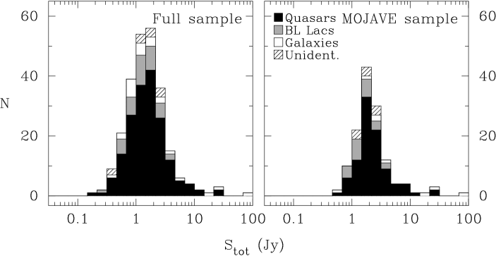
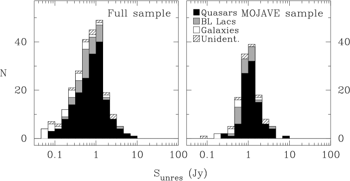
Figure 14.— Distribution of the flux density in the full and MOJAVE samples showing the median single antenna flux density $S_{\mathrm{tot}}$ (upper panel), and the median flux density of the most compact component $S_{\mathrm{unres}}$ (lower panel).

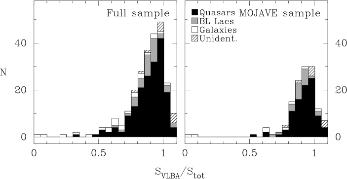
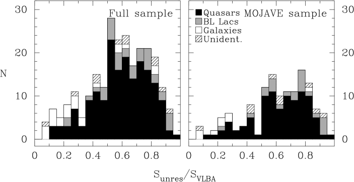
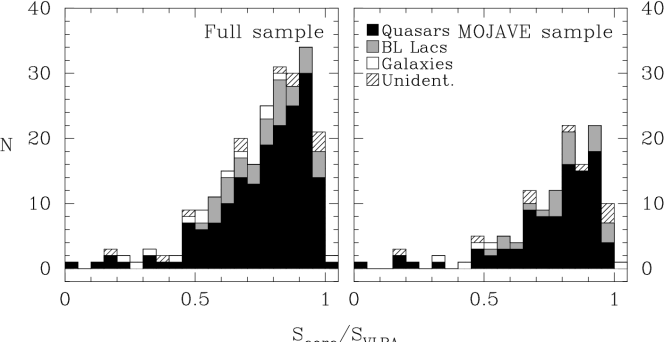
Figure 15.— Distributions of the median compactness indices on arcsecond scales $S_{\mathrm{VLBA}}/S_{\mathrm{tot}}$ (upper panel) and on sub-milliarcsecond scales $S_{\mathrm{unres}}/S_{\mathrm{VLBA}}$ (middle panel) as well as the VLBA core dominance $S_{\mathrm{core}}/S_{\mathrm{VLBA}}$ (lower panel). A few sources have an apparent compactness index at arcsecond scales $S_{\mathrm{VLBA}}/S_{\mathrm{tot}}>1$; this is due to source variability and the non-simultaneity of the VLBA and single antenna observations.

Figure 14 shows the distributions in our sample of the total flux densities, $S_{\mathrm{tot}}$, from single dish measurements, and the correlated flux densities, $S_{\mathrm{unres}}$, from long VLBA spacings. The peak in the distribution of $S_{\mathrm{tot}}$ corresponds to our nominal flux density limit of 1.5 or 2 Jy (depending on declination). The tail to lower flux densities in both panels is due to variability, and in the full sample (left hand panel) the tail also includes some sources of particular interest, which we included in the observations, but which did not meet our flux density criteria. Figure 15 gives the distributions of the “indices of compactness” on arcsecond scales, $S_{\mathrm{VLBA}}/S_{\mathrm{tot}}$, and sub-mas scales, $S_{\mathrm{unres}}/S_{\mathrm{VLBA}}$, as well as of the VLBA core dominance, $S_{\mathrm{core}}/S_{\mathrm{VLBA}}$.

Many sources in our sample have considerable flux on spatial scales sampled by the longest VLBA baselines. In the lower left hand panel of Figure 14, we see that more than 90% of the sources have an unresolved flux density greater than 0.1 Jy at projected baselines longer than 360 million wavelengths, while the middle left panel of Figure 15 shows that 68% of the sources have a median $S_{\mathrm{unres}}/S_{\mathrm{VLBA}}>0.5$. Table 2 lists, for each source, flux densities and model fitting results (as well as some other data) at the epoch for which its unresolved flux density $S_{\mathrm{unres}}$ was greatest. These data will be of value for various purposes, including planning future VLBI observations using Earth-space baselines. For 163 of these sources, the median flux density of the most compact component is greater than 0.5 Jy.

We have compared the measured values of $S_{\mathrm{VLBA}}$ and $S_{\mathrm{tot}}$. Figure 15 indicates that there are no significant systematic errors in the independently-constructed VLBA/RATAN/UMRAO flux density scales. The median compactness index on arcsecond scales, $S_{\mathrm{VLBA}}/S_{\mathrm{tot}}$, is 0.91 for the full sample and 0.93 for the MOJAVE sample, which indicates that for most sources the VLBA image contains nearly all of the flux density. Some sources have an apparent compactness on arcsecond scales $S_{\mathrm{VLBA}}/S_{\mathrm{tot}}>1$. Most likely, this is due to source variability and the non-simultaneity of the VLBA and single antenna observations. Sources with compactness index close to unity (see Table 2) are well-suited as calibrators for other VLBA observations.

5.2. Source Classes

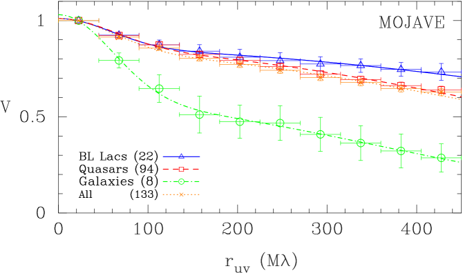
Figure 16.— The non-weighted mean of the fringe visibility versus projected spacing for the MOJAVE sample. The distribution is normalized to 1.0 at 25 million wavelengths. Visibility data at the epoch with the maximum correlated flux density at maximum VLBA spacings for each source is used. Before averaging over the samples, the fringe visibility amplitude for each source was binned and averaged. Vertical bars represent the $\pm 1\sigma$ formal error, horizontal bars — intervals of visibility data (ten bins in total). The lines represent the best fitting two-component models. See model parameters in Table 3.

The curves in Figure 16 show the mean visibility amplitude versus projected ($u$,$v$) spacing, averaged over all sources in the MOJAVE sample, and averaged over the MOJAVE quasars, BL Lacs, and active galaxies, separately. The best fitting parameter values for a model consisting of two Gaussian components are listed in Table 3 for each of these mean visibility curves.

The active galaxies are, on average, the least VLBA core dominated and the least compact on arcsecond (Figure 15) and sub-mas (Figures 15 and 16, and Table 3) scales. The fact that the relative contribution of an extended component (i.e. a jet) is significantly greater for active galaxies is consistent with unification models in which radio galaxies are viewed at larger angles to the line of sight than BL Lacs or quasars (e.g., Antonucci et al. 1987, Antonucci 1993, Urry & Padovani 1995, Wills 1999), so that the latter have higher Doppler factors, their cores are more boosted, and thus they appear more core dominated. The Kolmogorov-Smirnov (K-S) test confirms that for both the full and the MOJAVE sample the probability is less than 1% that the active galaxies have the same parent distribution as the quasars or the BL Lacs with regard to their compactness on arcsecond scales, $S_{\mathrm{VLBA}}/S_{\mathrm{tot}}$, or their compactness on sub-mas scales, $S_{\mathrm{unres}}/S_{\mathrm{VLBA}}$; with regard to their core dominance, $S_{\mathrm{core}}/S_{\mathrm{VLBA}}$, the probability is less than 2%.

For the BL Lacs versus quasars, K-S tests were inconclusive. However, Figure 16 and Table 3 show that the BL Lacs are, on average, even more compact on sub-mas scales than the quasars. We have also found this distinction between sub-samples of quasars and BL Lacs chosen to have statistically indistinguishable redshift distributions. The differences between the quasars and the BL Lacs in angular size at sub-mas scales in the sample as a whole are therefore not related to the different overall redshift distributions of these groups. As discussed in § 2, classifying objects is a complex issue, particularly with regard to BL Lacs. With our tabulated data, others could repeat the analysis using their own classification procedure if desired. However, the optical classification scheme we have used is evidently “clean” enough that, after the fact, it turns out to correspond to differences in radio compactness. We cannot image any hypothetical optical classification bias which could be fully responsible for the correspondence with radio compactness, and we conclude that it is an actual physical phenomenon.

Our sample does not show a significant dependence on redshift of the index of compactness on sub-mas scales, $S_{\mathrm{unres}}/S_{\mathrm{VLBA}}$, although the few heavily resolved sources are mostly active galaxies at low redshift.

5.3. Frequency Dependence

Horiuchi et al. (2004) have presented a plot, similar to Figure 16, based on 5 GHz VLBA and VSOP observations of 189 radio sources which cover a comparable range of spatial frequencies as our 15 GHz VLBA data. They find that the average fringe visibility in the range 400 to 440 million wavelengths is 0.21–0.24. For the 116 sources in common to the two samples (see Table 1), we find an average fringe visibility at 15 GHz of about 0.6. The compact component emission dominates at 15 GHz ($>$75%, see Table 3), but not at 5 GHz (40%, Horiuchi et al. 2004). This reflects the fact that the 5 GHz observations detect a larger contribution from steep spectrum optically thin large scale components. The 5 GHz VSOP survey sample and our 15 GHz VLBA sample are not identical, but this result is confirmed if only the subset of overlapping Pearson–Readhead VSOP survey sources (Lister et al. 2001, Horiuchi et al. 2004) is used for comparison.

5.4. Brightness Temperatures

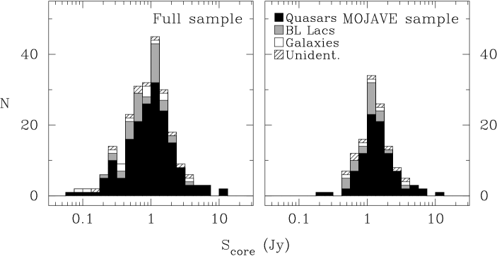
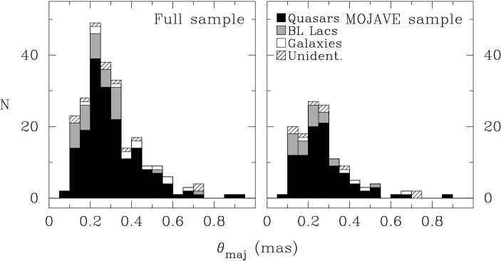
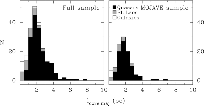
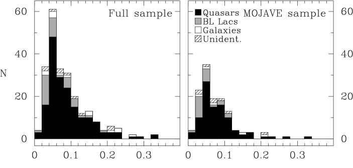
Figure 17.— From top to bottom, the distributions of the median flux density, angular and linear dimensions of core model components derived from the multi-epoch observations for each source.

Figure 18.— Distributions of the difference between the position angle of the major axis of the core and the position angle of a jet (left) and the difference between the position angle of the major axis of the core and the position angle of the major axis of the VLBA beam (right) for all the data modeled.

Figure 17 shows distributions of the core parameters. The ratio of the major axis of the core to the beam width in the same direction varies by more than an order of magnitude, so, in most cases, we believe that our measured core dimensions are not an artifact of the finite beam size.

The cores are always resolved along their major axis. However, for 158 sources in our full sample, there is at least one epoch at which the core component appears unresolved along the minor axis, where it is then typically less than 0.05 mas in size. In 19 of these sources, including 5 BL Lacs, the core is unresolved along the minor axis at all observed epochs.

Figure 18 shows the distribution of the difference between the position angle of the major axis of the core, $\mathrm{PA}_{\mathrm{core}}$, and the jet direction, $\mathrm{PA}_{\mathrm{jet}}$; the latter was taken to be the median over all epochs of the position angle of the jet component with respect to the core. All possible values of $|\mathrm{PA_{core}}-\mathrm{PA_{jet}}|$ between $0^{\circ}$ and $90^{\circ}$ are observed. Not unexpectedly, the peak of the distribution is close to zero; that is, the Gaussian component representing the core is typically extended along the jet direction. For the majority of sources which have multi-epoch modeling data, the orientation of the core is stable in time, with a scatter around the average $\mathrm{PA}_{\mathrm{core}}$ of less than $10^{\circ}$. Figure 18 also demonstrates that the position angle of the core is not correlated with the position angle of the VLBA beam, so that the measured core orientation is, in most cases, not distorted by the orientation of the VLBA beam.

The brightness temperature of a slightly resolved component in the rest frame of the source is given by

$$T_{\mathrm{b}}=\frac{2\,\ln 2}{\pi k}\frac{S_{\mathrm{core}}\,\lambda^{2}\,(1+z)}{\theta_{\mathrm{maj}}\,\theta_{\mathrm{min}}}\,,$$ (3)

where $S_{\mathrm{core}}$ is the flux density of a VLBA core, $\theta_{\mathrm{maj}}$ and $\theta_{\mathrm{min}}$ are the full width at half maximum (FWHM) of an elliptical Gaussian component along the major and the minor axis, $\lambda$ is the wavelength of observation, $z$ is the redshift, and $k$ is the Boltzmann constant. Observing at $\lambda=2$ cm with $S_{\mathrm{core}}$ measured in Jy, and $\theta_{\mathrm{maj}}$ and $\theta_{\mathrm{min}}$ in mas, we can write

$$T_{\mathrm{b}}=5.44\,\times\,10^{9}\,\frac{S_{\mathrm{core}}\,(1+z)}{\theta_{\mathrm{maj}}\,\theta_{\mathrm{min}}}\quad\mathrm{K}\,.$$ (4)

The brightness temperature can also be represented in terms of an effective baseline $D=\lambda/\sqrt{\theta_{\mathrm{maj}}\theta_{\mathrm{min}}}$. If $D$ is measured in km and $S_{\mathrm{core}}$ in Jy, we have

$$T_{\mathrm{b}}=3.20\,\times\,10^{2}\,S_{\mathrm{core}}\,D^{2}\,(1+z)\quad\mathrm{K}\,,$$ (5)

which is independent of wavelength and depends only on the physical length of the effective projected baseline and on the core flux density. For sources without measured redshift (see Table 1) we use $z=0$ to define a limit to $T_{\mathrm{b}}$.

Figure 19.— Distributions of the maximum observed VLBA core brightness temperature in the source frame. Each bin covers a factor of two in brightness temperature.

Paper I and Paper II gave conservative estimates of the observed peak brightness temperature based on the observed angular size, which is the intrinsic size convolved with the VLBA beam width. Here, we derive the core brightness temperature using the dimensions or upper limits obtained from direct modeling of the complex visibility functions. For many sources, the effective resolution is an order of magnitude better than given by Paper I and Paper II, so the corresponding derived brightness temperatures are as much as a factor of 100 greater. The median value of these VLBA core brightness temperatures, shown in Figure 19, is near $10^{12}$ K; they extend up to $5\,\times\,10^{13}$ K. This is comparable with brightness temperatures derived from VSOP space VLBI observations (Hirabayashi et al. 2000, Frey et al. 2000, Tingay et al. 2001, Horiuchi et al. 2004). In many cases our measurement refers only to the upper limit of the angular size, corresponding to our minimum resolvable size derived using equation (2). The effective resolution depends on the maximum baseline and on the signal-to-noise ratio near the maximum resolution. The true brightness temperatures of many sources may extend to a much higher value, beyond the equipartition value of $10^{11}$ K (Readhead 1994, Singal & Gopal-Krishna 1985) or the inverse Compton limit of $10^{12}$ K (Kellermann & Pauliny-Toth 1969). These high brightness temperatures are probably due to Doppler boosting, but transient non-equilibrium events, coherent emission, emission by relativistic protons, or a combination of these effects (e.g., Kardashev 2000, Kellermann 2002, 2003) may also play a role.

Figure 20.— Apparent velocity, $\beta_{\mathrm{max}}$, from Paper III versus maximum core brightness temperature, $T_{\mathrm{b,max}}$. Values of $\beta_{\mathrm{max}}$ are taken for the fastest components with ratings ‘E’ or ‘G’ only. Lower limits of brightness temperature are plotted as arrows. The curve is plotted for $T_{\mathrm{b,max}}=\beta_{\mathrm{max}}T_{\mathrm{int}}$, where the intrinsic brightness temperature is taken as $T_{\mathrm{int}}=10^{11}$ K.

If the high observed brightness temperatures are due to Doppler boosting, and if the range of intrinsic brightness temperatures, $T_{\mathrm{int}}$, is small, there should be a correlation between the apparent jet velocity, $\beta_{\mathrm{app}}$, and the observed brightness temperature. For those sources listed in Paper III, Figure 20 shows the fastest observed jet velocity against the maximum observed brightness temperature of their core. While this plot contains mostly lower limits to the brightness temperature, there are no sources with a low brightness temperature and a high observed speed; conversely, the highest speeds are observed only in sources with a high brightness temperature. This is the trend which we would expect if the observed brightness temperatures are Doppler boosted with $T_{\mathrm{obs}}=\delta T_{\mathrm{int}}$, where $\delta$ is the Doppler factor. At the optimum angle $\vartheta$ to the observer’s line of sight for superluminal motion, $\beta=\cos\vartheta$, $\beta_{\mathrm{app}}=\delta$ and therefore $T_{\mathrm{obs}}\simeq\beta_{\mathrm{app}}T_{\mathrm{int}}$. As shown in Figure 20, with $T_{\mathrm{int}}=10^{11}$ K, this curve tracks the trend of the data. Of course, the actual jet orientations deviate from the optimum viewing angle given by $\beta=\cos\vartheta$, and many of our brightness temperature estimates are lower limits. Both of these factors lead to a spread in the data, so we should not expect a tight correlation along the plotted line; however, the general agreement between the trend of the data and this simple model supports the idea that the intrinsic brightness temperatures have been Doppler boosted by the same relativistic motion that gives us the observed component speeds. We note that there are some sources with high brightness temperatures but low speeds. This is expected, as some sources will have an angle to the line of sight much smaller than $\beta=\cos\vartheta$, and those sources will have a small apparent motion but will still be highly beamed (M. H. Cohen et al., in preparation).

For those sources where there are multiple epochs of observation, the core parameters, in particular the observed brightness temperatures, vary significantly with time. Population modeling of the distribution of brightness temperature, as well as comparisons with the results of other VLBI surveys (e.g., Lobanov et al. 2000) may give insight into the distributions of intrinsic brightness temperatures and Doppler factors.

We have not found any significant correlation between redshift and brightness temperature. This is in agreement with the 5 GHz VSOP results of Horiuchi et al. (2004).

5.5. Variability

The long term cm-wave monitoring data on our sources from UMRAO and RATAN show complex light curves with frequent flux density outbursts (e.g., Aller et al. 2003, Kovalev et al. 2002). These outbursts are thought to be associated with the birth of new compact features, which are often not apparent in VLBI images until they have moved sufficiently far down the jet. Changes usually appear sooner in the visibility function (Figure 13), which in the case of our data, probes angular scales roughly 10 times smaller than the typical image restoring beam.

Most new jet features typically increase in size and/or decrease in flux density after a few months to years as a result of adiabatic expansion and/or synchrotron losses. However, an interesting exception is M 87 (1228+126), where the most compact feature appears to remain constant (Figure 13), although the larger scale jet structure shows changes by up to a factor of two in correlated flux density. This unusual behavior, which was first noted by Kellermann et al. (1973), is remarkable in that the dimensions of this compact stable feature are only of the order of ten lightdays or less. This weak ($\lesssim 0.2$ Jy) stable feature in the center of M 87 (catalog ) may be closely associated with the accretion region. More sensitive observations with comparable linear resolution might show similar phenomena in more distant sources, but such observations will only be possible with large antennas in space.

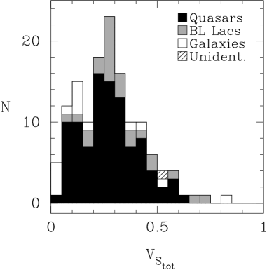
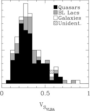
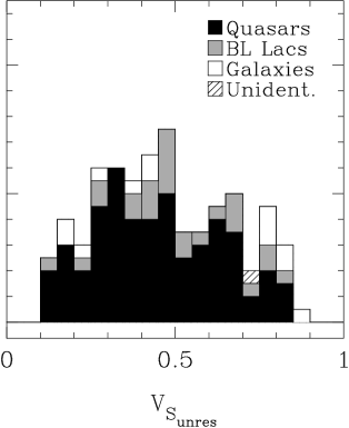
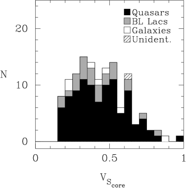
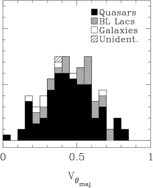
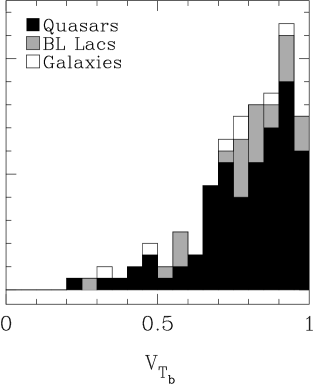
Figure 21.— Distributions of the variability index, $V$, derived for $S_{\mathrm{tot}}$, $S_{\mathrm{VLBA}}$, $S_{\mathrm{unres}}$, core flux density, major axis, and brightness temperature. The variability indices are calculated for 137 sources of the full sample observed four or more times.

We define a variability index as $V_{X}=\frac{X_{\mathrm{max}}-X_{\mathrm{min}}}{X_{\mathrm{max}}+X_{\mathrm{min}}}$. Figure 21 shows distributions of the variability indices $V_{S_{\mathrm{tot}}}$, $V_{S_{\mathrm{VLBA}}}$, and $V_{S_{\mathrm{unres}}}$, as well as, to represent the cores, $V_{S_{\mathrm{core}}}$, $V_{\theta_{\mathrm{maj}}}$, and $V_{T_{\mathrm{b}}}$. As expected, the variability indices for the flux density become larger with improved resolution, going from median values of $V_{S_{\mathrm{tot}}}=0.27$ and $V_{S_{\mathrm{VLBA}}}=0.30$ to $V_{S_{\mathrm{core}}}=0.42$ and $V_{S_{\mathrm{unres}}}=0.45$. For about 68% of the sources, the flux density of the core has varied by a factor of 2 or more, that is $V>1/3$. Similarly, the size of the core major axis, $\theta_{\mathrm{maj}}$, changed by as much as a factor of 5, or $V>2/3$, in some cases. Probably, this is due to the creation or ejection of a new component, which initially is not resolved from the core, but then separates from it, causing first an apparent increase, and then an apparent decrease in the strength and size of the core. The observed strong variability of the brightness temperatures (median $V_{T_{\mathrm{b}}}=0.82$) may reflect strong variations of particle density (due to ejections) and/or magnetic field strength. The most variable sources tend to have the most compact structure. A variability index $V_{S_{\mathrm{VLBA}}}>0.6$ is observed for nine sources, all but one of which have sub-mas compactness $S_{\mathrm{unres}}/S_{\mathrm{VLBA}}\geq 0.75$.

5.6. Intra-Day Variable Sources

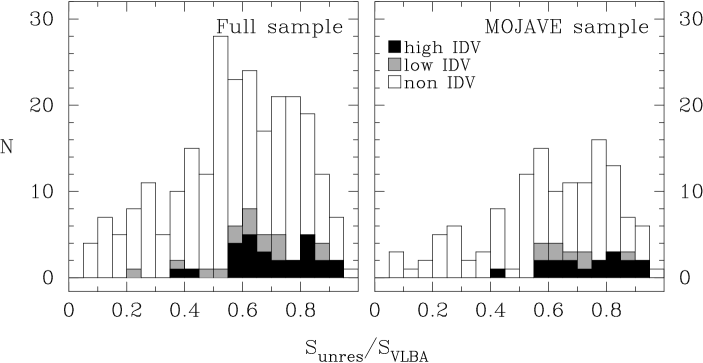
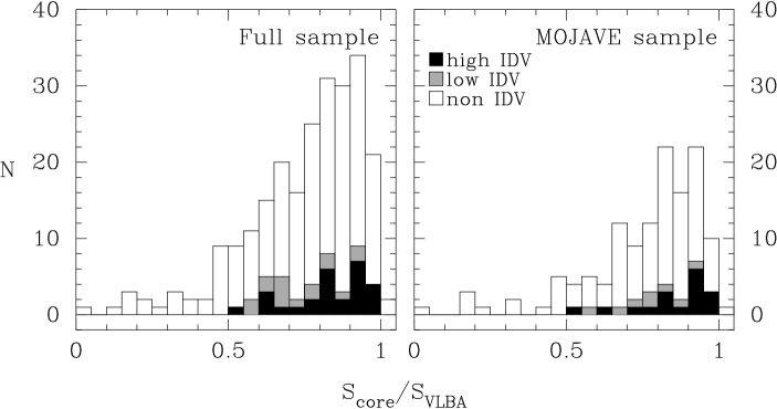
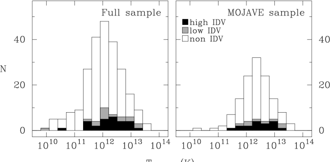
Figure 22.— Distributions of the median compactness index on sub-milliarcsecond scales $S_{\mathrm{unres}}/S_{\mathrm{VLBA}}$ (upper panels), the VLBA core dominance $S_{\mathrm{core}}/S_{\mathrm{VLBA}}$ (middle panels) and maximum brightness temperature $T_{\mathrm{b,max}}$ (lower panels) for IDV selected and non-selected sources. We separate IDVs with high modulation index ($m>0.02$ observed at least once — “high IDV”) from ones with low modulation index (measured values of modulation index always less than 0.02 or are not reported — “low IDV”).

We have used the results of several IDV search and monitoring programs at the Effelsberg 100 meter telescope, the VLA, and the ATCA at 1.4 to 15 GHz (Quirrenbach et al. 1992, 2000, Kedziora-Chudczer et al. 2001, Bignall et al. 2002, Kraus et al. 2003, Lovell et al. 2003), to identify IDV sources in our sample (Table 1). The biggest and most complete IDV survey so far, the 5 GHz MASIV survey (Lovell et al. 2003), started at the VLA in 2002; the first results reported by Lovell et al. suggest that 85 of 710 compact flat-spectrum sources are IDVs. The MASIV data, however, are not yet fully published. We have labeled a source in our sample as an IDV if there is a published statistically significant detection of flux density variations on a time scale of less that 3 days (72 hours). However, we are not able to identify all of the potential IDV sources in our sample consistently, because some sources are not (yet) listed in any of the published IDV survey results, and also because intra-day variability is a transient phenomenon, and not all sources were monitored equally well.

Figure 22 shows the distribution of the sub-mas compactness index, $S_{\mathrm{unres}}/S_{\mathrm{VLBA}}$; the median value over all observing epochs was taken for each source. The median VLBA core dominance, $S_{\mathrm{core}}/S_{\mathrm{VLBA}}$, and the maximum brightness temperature are also shown. The full and the MOJAVE sample are shown separately, and we have separated IDVs with high modulation index ($m>0.02$ observed at least once) from ones with low modulation index (measured values of modulation index always less than 0.02, or not reported).

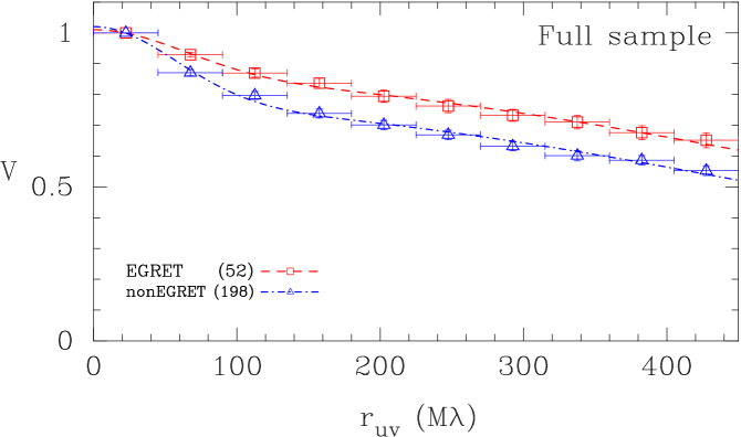
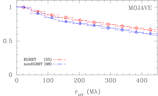
Figure 23.— The non-weighted mean of the fringe visibility versus projected spacing. The distribution is normalized to 1.0 at 25 million wavelengths. The visibility data at the epoch with the maximum correlated flux density $S_{\mathrm{unres}}$ is used for each source. The sample is divided into “gamma-ray bright” (EGRET detections) and “gamma-ray weak” (EGRET non-detections) sources (see Table 1 for details). The lines represent the best fitting two-component models. See model parameters in Table 3.

We find that IDV sources have more compact and more core dominant structure on sub-milliarcsecond scales (Table 4) than non-IDV sources. IDVs with a higher amplitude of intra-day variation tend to have a higher unresolved flux density, $S_{\mathrm{unres}}$. The results for core dominance are in agreement with previous findings (e.g., Witzel & Quirrenbach 1993, Ojha et al. 2004). A K-S test yields a probability of less than 1% for both the full and the MOJAVE sample that the sub-mas compactness (Figure 22) has the same parent distribution for IDV and non-IDV sources.

One might expect IDV behavior in almost all the sources with high visibility amplitude at long VLBI spacings. However, this was not observed by IDV surveys, perhaps because of the intermittent nature of the IDV phenomenon.

Some IDV observations have suggested apparent brightness temperatures up to $10^{15}$ K if they are due to interstellar scintillations, and up to $10^{21}$ K if they are intrinsic (e.g., Kedziora-Chudczer et al. 1997). More recently, IDV observations of Lovell et al. (2003) have shown typical brightness temperature values of the order of $10^{12}$ K, consistent with our results (Figure 22). However, as seen from equation (5), the highest brightness temperature which we can reliably discern is of the order of $10^{13}$ K, so we are not able to comment on the evidence for the extremely high brightness temperatures and the corresponding high Lorentz factors inferred for some IDV.

5.7. Gamma-ray Sources

The third catalog of high energy gamma-ray sources detected by the EGRET telescope of the Compton Gamma Ray Observatory (Hartman et al. 1999) includes 66 high-confidence identifications of blazars (Mattox et al. 2001, Sowards-Emmerd et al. 2003, 2004). While the gamma-ray sources were identified with flat-spectrum extragalactic radio sources ($\alpha>-0.5$, not all flat-spectrum sources have been detected as gamma-ray sources. This is not necessarily indicative of a bi-modality in the gamma-ray loudness distribution of extragalactic radio sources (such as that found at radio wavelengths), since the sensitivity level of EGRET was such that many sources were only detected in their flaring state. With the next generation of gamma-ray telescopes, such as GLAST (Gehrels & Michelson 1999), the sensitivity may be sufficient to actually separate the classes of gamma-ray loud and gamma-ray quiet objects and to define the relationship between radio and gamma-ray emission of the sources properly.

For the purpose of our test we have grouped the “highly probable” and “probable” EGRET identifications (Table 1) together, which yields 52 “EGRET detections” out of 250 objects for the full and 35 out of 133 for the MOJAVE sample.

In Paper I we did not find any clear differences in the sub-milliarcsecond scale structure between the EGRET (20% of our radio sample) and non-EGRET sources. However, we find here that the sub-mas compactness, $S_{\mathrm{unres}}/S_{\mathrm{VLBA}}$, for EGRET detections is, on average, greater than for the EGRET non-detections. This can be seen in Figure 23 which shows the mean visibility function amplitudes versus projected spacing for EGRET detected and non-detected sources, for the full and MOJAVE samples. For both samples, the EGRET detected sources have, on average, a higher contribution of compact VLBA structure (see Table 3 for the parameters of the two-component fit). This comparison is valid because the EGRET detected and non-detected blazars in our sample have indistinguishable redshift distributions. This result still holds if we exclude the GPS and steep spectrum sources, which are generally gamma-ray weak (see, e.g., Mattox et al. 1997). The difference is more pronounced for the full sample, which is not selected on the basis of the VLBI flux density. The difference for the MOJAVE sample is small, but remains significant. These results suggest that a connection may exist between gamma-ray and beamed radio emission from extragalactic sources on sub-milliarcsecond scales, as has already being argued by others (e.g., Jorstad et al. 2001).

6. Summary

We have analyzed visibility function data of 250 extragalactic radio sources, obtained with the VLBA at 15 GHz. Almost all of the radio sources in our sample have unresolved radio emission brighter than 0.1 Jy on the longest VLBA baselines. For 171 objects, more than half of the flux density comes from unresolved features. We have compiled a list of 163 sources with unresolved structure stronger than 0.5 Jy, which will form a target list of special interest for planned space VLBI observations such as RadioAstron, VSOP–2, and ARISE.

A few of the sources have an overall radio structure which is only slightly resolved at the longest spacings. Their total angular size is less than about 0.05 mas, at least in one dimension, at some epochs. However, even though most sources in our full sample are extended overall, there are 158 sources in which the VLBA core component appears unresolved, usually smaller than 0.05 mas, again in one direction, at least at one epoch. For 19 of these, the core was unresolved at all epochs.

The distribution of the brightness temperature of the cores peaks at $10^{12}$ K and extends up to $5\,\times\,10^{13}$ K; this is close to the limit set by the dimensions of the VLBA. However, for many sources we only measure a lower limit to the brightness temperature. There is evidence that the observed brightness temperatures can be explained as the result of Doppler boosting, but transient phenomena, coherent emission, or synchrotron emission by relativistic protons may also be important.

On sub-milliarcsecond scales, active galaxies are on average larger and less core dominated than quasars, which is consistent with unification models in which the latter are viewed at smaller angles to the line of sight. Additionally, the weak-lined objects classified as BL Lacs tend to be smaller than the broad-lined quasars in our sample. IDV sources show a higher compactness and core dominance on sub-mas scales than non-IDV ones. IDVs with a higher amplitude of intra-day variation tend to have a higher flux density in an unresolved component. The most variable sources tend to have the most compact structure. EGRET-detected radio sources show a higher degree of sub-mas compactness than non-EGRET sources, supporting emission models which relate the radio and gamma-ray emission, such as inverse Compton scattering (see, e.g., Bloom & Marscher 1996).

Table 1 General Source Properties

IAU		R.A.	Dec.	Opt.		Radio	EGRET	MOJAVE	VSOP	IDV
Name	Alias	(J2000.0)	(J2000.0)	Class	$z$	Spectrum	ID	Member	Sample	Ref.
(1)	(2)	(3)	(4)	(5)	(6)	(7)	(8)	(9)	(10)	(11)
0003$-$066	NRAO 5	00 06 13.8929	$-$06 23 35.3353	B	0.347	Flat	$\cdots$	Y	A	$\cdots$
0007$+$106	III Zw 2	00 10 31.0059	$+$10 58 29.5041	G	0.089	Flat	$\cdots$	Y	$\cdots$	$\cdots$
0014$+$813		00 17 08.4750	$+$81 35 08.1360	Q	3.387	Flat	$\cdots$	$\cdots$	$\cdots$	$\cdots$
0016$+$731		00 19 45.7864	$+$73 27 30.0175	Q	1.781	Flat	$\cdots$	Y	A, PR	$\cdots$
0026$+$346		00 29 14.2425	$+$34 56 32.2466	G	0.517	Flat	$\cdots$	$\cdots$	C	$\cdots$
0035$+$413		00 38 24.8436	$+$41 37 06.0006	Q	1.353	Flat	$\cdots$	$\cdots$	C	$\cdots$
0039$+$230		00 42 04.5451	$+$23 20 01.0610	U	$\cdots$	Peaked	$\cdots$	$\cdots$	A	$\cdots$
0048$-$097		00 50 41.3174	$-$09 29 05.2102	B	$\cdots$	Flat	$\cdots$	Y	$\cdots$	$\cdots$
0055$+$300	NGC 315	00 57 48.8834	$+$30 21 08.8119	G	0.016	Flat	$\cdots$	$\cdots$	$\cdots$	$\cdots$
0059$+$581		01 02 45.7624	$+$58 24 11.1366	U	$\cdots$	Flat	$\cdots$	Y	$\cdots$	5,6
0106$+$013		01 08 38.7711	$+$01 35 00.3171	Q	2.107	Flat	$\cdots$	Y	B	$\cdots$
0108$+$388		01 11 37.3192	$+$39 06 27.9986	G	0.669	Peaked	$\cdots$	$\cdots$	C	$\cdots$
0109$+$224		01 12 05.8247	$+$22 44 38.7862	B	$\cdots$	Flat	$\cdots$	Y	$\cdots$	$\cdots$
0112$-$017		01 15 17.1000	$-$01 27 04.5772	Q	1.365	Flat	$\cdots$	$\cdots$	A	$\cdots$
0113$-$118		01 16 12.5220	$-$11 36 15.4340	Q	0.672	Flat	$\cdots$	$\cdots$	A	$\cdots$
0119$+$041		01 21 56.8617	$+$04 22 24.7344	Q	0.637	Flat	NP	$\cdots$	A	$\cdots$
0119$+$115	OC +131	01 21 41.5950	$+$11 49 50.4131	Q	0.570	Flat	$\cdots$	Y	A	$\cdots$
0122$-$003		01 25 28.8427	$-$00 05 55.9630	Q	1.070	Flat	$\cdots$	$\cdots$	A	$\cdots$
0133$-$203		01 35 37.5086	$-$20 08 45.8870	Q	1.141	Flat	$\cdots$	$\cdots$	$\cdots$	$\cdots$
0133$+$476	DA 55	01 36 58.5948	$+$47 51 29.1001	Q	0.859	Flat	$\cdots$	Y	A, PR	1
0138$-$097		01 41 25.8320	$-$09 28 43.6730	B	0.733	Flat	$\cdots$	$\cdots$	B	$\cdots$
0146$+$056		01 49 22.3709	$+$05 55 53.5680	Q	2.345	Flat	$\cdots$	$\cdots$	A	$\cdots$
0149$+$218		01 52 18.0590	$+$22 07 07.7000	Q	1.32	Flat	$\cdots$	$\cdots$	B	$\cdots$
0153$+$744		01 57 34.9649	$+$74 42 43.2300	Q	2.341	Flat	$\cdots$	$\cdots$	C, PR	$\cdots$
0201$+$113		02 03 46.6571	$+$11 34 45.4096	Q	3.61	Peaked	$\cdots$	$\cdots$	$\cdots$	$\cdots$
0202$+$149	4C +15.05	02 04 50.4139	$+$15 14 11.0435	Q	0.405	Flat	YY	Y	B	$\cdots$
0202$+$319		02 05 04.9254	$+$32 12 30.0956	Q	1.466	Flat	$\cdots$	Y	B	$\cdots$
0212$+$735		02 17 30.8134	$+$73 49 32.6218	Q	2.367	Flat	$\cdots$	Y	A, PR	$\cdots$
0215$+$015		02 17 48.9547	$+$01 44 49.6991	B	1.715	Flat	$\cdots$	Y	A	$\cdots$
0218$+$357		02 21 05.4740	$+$35 56 13.7315	Q	0.944	Flat	$\cdots$	$\cdots$	C	$\cdots$
0221$+$067	4C +07.11	02 24 28.4282	$+$06 59 23.3416	Q	0.511	Flat	$\cdots$	$\cdots$	B	$\cdots$
0224$+$671	4C +67.05	02 28 50.0515	$+$67 21 03.0293	U	$\cdots$	Flat	$\cdots$	Y	$\cdots$	$\cdots$
0234$+$285	CTD 20	02 37 52.4057	$+$28 48 08.9901	Q	1.207	Flat	YP	Y	B	$\cdots$
0235$+$164		02 38 38.9301	$+$16 36 59.2747	B	0.940	Flat	YY	Y	C	1,2,6
0238$-$084	NGC 1052	02 41 04.7985	$-$08 15 20.7518	G	0.005	Flat	$\cdots$	Y	C	$\cdots$
0248$+$430		02 51 34.5368	$+$43 15 15.8290	Q	1.310	Flat	$\cdots$	$\cdots$	A	$\cdots$
0300$+$470	4C +47.08	03 03 35.2422	$+$47 16 16.2755	B	$\cdots$	Flat	$\cdots$	Y	$\cdots$	$\cdots$
0310$+$013		03 12 43.6028	$+$01 33 17.5380	Q	0.664	Flat	$\cdots$	$\cdots$	B	$\cdots$
0316$+$162	CTA 21	03 18 57.8016	$+$16 28 32.7048	G	$\cdots$	Peaked	$\cdots$	$\cdots$	$\cdots$	$\cdots$
0316$+$413	3C 84	03 19 48.1601	$+$41 30 42.1031	G	0.017	Flat	$\cdots$	Y	A, PR	$\cdots$
0333$+$321	NRAO 140	03 36 30.1076	$+$32 18 29.3424	Q	1.263	Flat	$\cdots$	Y	B	2
0336$-$019	CTA 26	03 39 30.9378	$-$01 46 35.8040	Q	0.852	Flat	YY	Y	A	2
0355$+$508	NRAO 150	03 59 29.7473	$+$50 57 50.1615	Q	$\cdots$	Flat	$\cdots$	$\cdots$	$\cdots$	$\cdots$
0402$-$362		04 03 53.7499	$-$36 05 01.9120	Q	1.417	Peaked	$\cdots$	$\cdots$	A	$\cdots$
0403$-$132		04 05 34.0034	$-$13 08 13.6911	Q	0.571	Flat	$\cdots$	Y	A	$\cdots$
0405$-$385		04 06 59.0353	$-$38 26 28.0421	Q	1.285	Flat	$\cdots$	$\cdots$	B	3
0415$+$379	3C 111	04 18 21.2770	$+$38 01 35.9000	G	0.049	Steep	$\cdots$	Y	$\cdots$	$\cdots$
0420$-$014		04 23 15.8007	$-$01 20 33.0653	Q	0.915	Flat	YY	Y	A	$\cdots$
0420$+$022		04 22 52.2146	$+$02 19 26.9319	Q	2.277	Flat	$\cdots$	$\cdots$	$\cdots$	$\cdots$
0422$+$004		04 24 46.8421	$+$00 36 06.3298	B	$\cdots$	Flat	$\cdots$	Y	A	3
0429$+$415	3C 119	04 32 36.5026	$+$41 38 28.4485	Q	1.023	Steep	$\cdots$	$\cdots$	$\cdots$	$\cdots$
0430$+$052	3C 120	04 33 11.0955	$+$05 21 15.6194	G	0.033	Flat	$\cdots$	Y	A	$\cdots$
0438$-$436		04 40 17.1800	$-$43 33 08.6030	Q	2.852	Flat	$\cdots$	$\cdots$	$\cdots$	$\cdots$
0440$-$003	NRAO 190	04 42 38.6608	$-$00 17 43.4191	Q	0.844	Flat	YP	$\cdots$	$\cdots$	3
0446$+$112		04 49 07.6711	$+$11 21 28.5966	Q	$\cdots$	Flat	PY	Y	B	$\cdots$
0454$-$234		04 57 03.1792	$-$23 24 52.0180	B	1.003	Flat	YY	$\cdots$	A	$\cdots$
0454$+$844		05 08 42.3635	$+$84 32 04.5440	B	$>$1.34	Flat	$\cdots$	$\cdots$	B	4
0458$-$020		05 01 12.8099	$-$01 59 14.2562	Q	2.291	Flat	YY	Y	A	$\cdots$
0521$-$365		05 22 57.9846	$-$36 27 30.8516	G	0.055	Steep	$\cdots$	$\cdots$	$\cdots$	$\cdots$
0524$+$034		05 27 32.7030	$+$03 31 31.4500	B	$\cdots$	Flat	$\cdots$	$\cdots$	$\cdots$	$\cdots$
0528$+$134		05 30 56.4167	$+$13 31 55.1495	Q	2.07	Flat	YY	Y	B	$\cdots$
0529$+$075		05 32 38.9985	$+$07 32 43.3459	U	$\cdots$	Flat	$\cdots$	Y	C	$\cdots$
0529$+$483		05 33 15.8658	$+$48 22 52.8078	Q	1.162	Flat	PY	Y	$\cdots$	$\cdots$
0537$-$286		05 39 54.2814	$-$28 39 55.9460	Q	3.104	Flat	NP	$\cdots$	A	$\cdots$
0552$+$398	DA 193	05 55 30.8056	$+$39 48 49.1650	Q	2.363	Peaked	$\cdots$	Y	$\cdots$	$\cdots$
0602$+$673		06 07 52.6716	$+$67 20 55.4098	Q	1.97	Flat	$\cdots$	$\cdots$	B	4
0605$-$085	OH $-$010	06 07 59.6992	$-$08 34 49.9781	Q	0.872	Flat	$\cdots$	Y	A	$\cdots$
0607$-$157		06 09 40.9495	$-$15 42 40.6726	Q	0.324	Flat	$\cdots$	Y	A	3
0615$+$820		06 26 03.0062	$+$82 02 25.5676	Q	0.71	Flat	$\cdots$	$\cdots$	B	$\cdots$
0642$+$449	OH 471	06 46 32.0260	$+$44 51 16.5901	Q	3.408	Peaked	$\cdots$	Y	B	$\cdots$
0648$-$165		06 50 24.5819	$-$16 37 39.7250	U	$\cdots$	Flat	$\cdots$	Y	$\cdots$	$\cdots$
0707$+$476		07 10 46.1049	$+$47 32 11.1427	Q	1.292	Flat	$\cdots$	$\cdots$	$\cdots$	$\cdots$
0710$+$439		07 13 38.1641	$+$43 49 17.2051	G	0.518	Peaked	$\cdots$	$\cdots$	B	$\cdots$
0711$+$356	OI 318	07 14 24.8175	$+$35 34 39.7950	Q	1.620	Peaked	$\cdots$	$\cdots$	A, PR	1
0716$+$714		07 21 53.4485	$+$71 20 36.3634	B	$\cdots$	Flat	YY	Y	$\cdots$	1,2,4,6
0723$-$008		07 25 50.6400	$-$00 54 56.5444	B	0.127	Flat	$\cdots$	$\cdots$	$\cdots$	$\cdots$
0727$-$115		07 30 19.1125	$-$11 41 12.6005	Q	1.591	Flat	$\cdots$	Y	$\cdots$	$\cdots$
0730$+$504		07 33 52.5206	$+$50 22 09.0621	Q	0.720	Flat	$\cdots$	Y	$\cdots$	$\cdots$
0735$+$178		07 38 07.3937	$+$17 42 18.9983	B	$>$0.424	Flat	YY	Y	A	1
0736$+$017		07 39 18.0339	$+$01 37 04.6180	Q	0.191	Flat	$\cdots$	Y	A	$\cdots$
0738$+$313	OI 363	07 41 10.7033	$+$31 12 00.2286	Q	0.630	Flat	$\cdots$	Y	A	$\cdots$
0742$+$103		07 45 33.0595	$+$10 11 12.6925	Q	2.624	Peaked	$\cdots$	Y	B	$\cdots$
0745$+$241		07 48 36.1093	$+$24 00 24.1102	Q	0.409	Flat	$\cdots$	$\cdots$	A	$\cdots$
0748$+$126		07 50 52.0457	$+$12 31 04.8282	Q	0.889	Flat	$\cdots$	Y	B	$\cdots$
0754$+$100		07 57 06.6429	$+$09 56 34.8521	B	0.266	Flat	$\cdots$	Y	$\cdots$	5,6
0804$+$499	OJ 508	08 08 39.6663	$+$49 50 36.5305	Q	1.432	Flat	$\cdots$	Y	B	1,2,4,6
0805$-$077		08 08 15.5360	$-$07 51 09.8863	Q	1.837	Flat	$\cdots$	Y	C	$\cdots$
0808$+$019		08 11 26.7073	$+$01 46 52.2200	B	0.93	Flat	$\cdots$	Y	A	3
0814$+$425	OJ 425	08 18 15.9996	$+$42 22 45.4149	B	$\cdots$	Flat	$\cdots$	Y	A, PR	1
0821$+$394	4C +39.23	08 24 55.4839	$+$39 16 41.9043	Q	1.216	Flat	$\cdots$	$\cdots$	B	$\cdots$
0823$+$033		08 25 50.3384	$+$03 09 24.5201	B	0.506	Flat	$\cdots$	Y	A	$\cdots$
0827$+$243		08 30 52.0862	$+$24 10 59.8205	Q	0.941	Flat	YY	Y	$\cdots$	$\cdots$
0829$+$046		08 31 48.8770	$+$04 29 39.0853	B	0.18	Flat	YY	Y	B	$\cdots$
0831$+$557	4C +55.16	08 34 54.9041	$+$55 34 21.0710	G	0.240	Flat	$\cdots$	$\cdots$	C	$\cdots$
0834$-$201		08 36 39.2152	$-$20 16 59.5035	Q	2.752	Flat	$\cdots$	$\cdots$	$\cdots$	$\cdots$
0836$+$710	4C +71.08	08 41 24.3653	$+$70 53 42.1731	Q	2.218	Flat	YY	Y	A, PR	$\cdots$
0838$+$133	3C 207	08 40 47.6848	$+$13 12 23.8790	Q	0.684	Flat	$\cdots$	$\cdots$	B	$\cdots$
0850$+$581	4C +58.17	08 54 41.9964	$+$57 57 29.9393	Q	1.322	Flat	$\cdots$	$\cdots$	B	$\cdots$
0851$+$202	OJ 287	08 54 48.8749	$+$20 06 30.6409	B	0.306	Flat	YY	Y	A	$\cdots$
0859$-$140		09 02 16.8309	$-$14 15 30.8757	Q	1.339	Steep	$\cdots$	$\cdots$	$\cdots$	$\cdots$
0859$+$470	4C +47.29	09 03 03.9901	$+$46 51 04.1375	Q	1.462	Steep	$\cdots$	$\cdots$	A, PR	$\cdots$
0906$+$015	4C +01.24	09 09 10.0916	$+$01 21 35.6177	Q	1.018	Flat	$\cdots$	Y	A	$\cdots$
0917$+$449		09 20 58.4585	$+$44 41 53.9851	Q	2.180	Flat	NP	$\cdots$	A	$\cdots$
0917$+$624		09 21 36.2311	$+$62 15 52.1804	Q	1.446	Flat	$\cdots$	Y	B	1,2,4
0919$-$260		09 21 29.3538	$-$26 18 43.3850	Q	2.300	Peaked	$\cdots$	$\cdots$	B	$\cdots$
0923$+$392	4C +39.25	09 27 03.0139	$+$39 02 20.8520	Q	0.698	Flat	$\cdots$	Y	A, PR	$\cdots$
0945$+$408	4C +40.24	09 48 55.3381	$+$40 39 44.5872	Q	1.252	Flat	$\cdots$	Y	B	$\cdots$
0953$+$254	OK 290	09 56 49.8754	$+$25 15 16.0498	Q	0.712	Flat	$\cdots$	$\cdots$	B	$\cdots$
0954$+$658		09 58 47.2451	$+$65 33 54.8181	B	0.367	Flat	YY	$\cdots$	B	1,2,4
0955$+$476	OK 492	09 58 19.6716	$+$47 25 07.8425	Q	1.873	Flat	$\cdots$	Y	B	6
1012$+$232	4C +23.24	10 14 47.0654	$+$23 01 16.5709	Q	0.565	Flat	$\cdots$	$\cdots$	B	6
1015$+$359		10 18 10.9877	$+$35 42 39.4380	Q	1.226	Flat	$\cdots$	$\cdots$	$\cdots$	$\cdots$
1032$-$199		10 35 02.1553	$-$20 11 34.3597	Q	2.198	Flat	$\cdots$	$\cdots$	A	$\cdots$
1034$-$293		10 37 16.0797	$-$29 34 02.8120	Q	0.312	Flat	$\cdots$	$\cdots$	A	3
1036$+$054		10 38 46.7799	$+$05 12 29.0854	U	$\cdots$	Flat	$\cdots$	Y	$\cdots$	$\cdots$
1038$+$064	4C +06.41	10 41 17.1625	$+$06 10 16.9238	Q	1.265	Flat	$\cdots$	Y	B	$\cdots$
1045$-$188		10 48 06.6206	$-$19 09 35.7270	Q	0.595	Flat	$\cdots$	Y	B	$\cdots$
1049$+$215	4C +21.28	10 51 48.7891	$+$21 19 52.3142	Q	1.300	Flat	$\cdots$	$\cdots$	B	$\cdots$
1055$+$018	4C +01.28	10 58 29.6052	$+$01 33 58.8237	Q	0.888	Flat	$\cdots$	Y	A	$\cdots$
1055$+$201	4C +20.24	10 58 17.9025	$+$19 51 50.9018	Q	1.11	Flat	$\cdots$	$\cdots$	B	$\cdots$
1101$+$384	Mrk 421	11 04 27.3139	$+$38 12 31.7991	B	0.031	Flat	YY	$\cdots$	$\cdots$	$\cdots$
1116$+$128		11 18 57.3014	$+$12 34 41.7180	Q	2.118	Flat	$\cdots$	$\cdots$	A	$\cdots$
1124$-$186	OM $-$148	11 27 04.3924	$-$18 57 17.4417	Q	1.048	Flat	$\cdots$	Y	B	$\cdots$
1127$-$145		11 30 07.0526	$-$14 49 27.3882	Q	1.187	Flat	$\cdots$	Y	$\cdots$	$\cdots$
1128$+$385		11 30 53.2826	$+$38 15 18.5470	Q	1.733	Flat	$\cdots$	$\cdots$	$\cdots$	$\cdots$
1144$+$402		11 46 58.2979	$+$39 58 34.3046	Q	1.089	Flat	$\cdots$	$\cdots$	$\cdots$	$\cdots$
1145$-$071		11 47 51.5540	$-$07 24 41.1411	Q	1.342	Flat	$\cdots$	$\cdots$	A	$\cdots$
1148$-$001	4C $-$00.47	11 50 43.8708	$-$00 23 54.2049	Q	1.980	Peak?	$\cdots$	$\cdots$	B	$\cdots$
1150$+$812		11 53 12.4991	$+$80 58 29.1545	Q	1.25	Flat	$\cdots$	Y	B	1
1155$+$251		11 58 25.7875	$+$24 50 17.9640	Q	0.202	Flat	$\cdots$	$\cdots$	C	$\cdots$
1156$+$295	4C +29.45	11 59 31.8339	$+$29 14 43.8269	Q	0.729	Flat	YP	Y	B	5,6
1213$-$172		12 15 46.7518	$-$17 31 45.4029	U	$\cdots$	Flat	$\cdots$	Y	A	$\cdots$
1219$+$044	ON +231	12 22 22.5496	$+$04 13 15.7763	Q	0.965	Flat	$\cdots$	Y	$\cdots$	$\cdots$
1219$+$285	W Comae	12 21 31.6905	$+$28 13 58.5002	B	0.102	Flat	PP	$\cdots$	$\cdots$	$\cdots$
1222$+$216		12 24 54.4584	$+$21 22 46.3886	Q	0.435	Flat	YY	Y	B	$\cdots$
1226$+$023	3C 273	12 29 06.6997	$+$02 03 08.5982	Q	0.158	Flat	YY	Y	A	$\cdots$
1228$+$126	M87	12 30 49.4234	$+$12 23 28.0439	G	0.004	Steep	$\cdots$	Y	$\cdots$	$\cdots$
1244$-$255		12 46 46.8020	$-$25 47 49.2880	Q	0.638	Flat	$\cdots$	$\cdots$	A	$\cdots$
1253$-$055	3C 279	12 56 11.1666	$-$05 47 21.5246	Q	0.538	Flat	YY	Y	A	$\cdots$
1255$-$316		12 57 59.0608	$-$31 55 16.8520	Q	1.924	Flat	$\cdots$	$\cdots$	A	$\cdots$
1302$-$102		13 05 33.0150	$-$10 33 19.4282	Q	0.286	Flat	$\cdots$	$\cdots$	A	$\cdots$
1308$+$326		13 10 28.6638	$+$32 20 43.7830	Q	0.997	Flat	$\cdots$	Y	A	$\cdots$
1313$-$333		13 16 07.9859	$-$33 38 59.1720	Q	1.21	Flat	NP	$\cdots$	A	$\cdots$
1323$+$321	4C +32.44	13 26 16.5122	$+$31 54 09.5154	G	0.370	Peaked	$\cdots$	$\cdots$	$\cdots$	$\cdots$
1324$+$224		13 27 00.8613	$+$22 10 50.1631	Q	1.40	Flat	NP	Y	$\cdots$	$\cdots$
1328$+$307	3C 286	13 31 08.2880	$+$30 30 32.9588	Q	0.846	Steep	$\cdots$	$\cdots$	$\cdots$	$\cdots$
1334$-$127		13 37 39.7828	$-$12 57 24.6932	Q	0.539	Flat	YY	Y	A	$\cdots$
1345$+$125	4C +12.50	13 47 33.3616	$+$12 17 24.2390	G	0.121	Peaked	$\cdots$	$\cdots$	C	$\cdots$
1354$-$152		13 57 11.2450	$-$15 27 28.7864	Q	1.890	Flat	$\cdots$	$\cdots$	$\cdots$	$\cdots$
1354$+$195	DA 354	13 57 04.4368	$+$19 19 07.3640	Q	0.719	Flat	$\cdots$	$\cdots$	A	$\cdots$
1402$+$044		14 05 01.1198	$+$04 15 35.8190	Q	3.211	Flat	$\cdots$	$\cdots$	B	$\cdots$
1404$+$286	OQ 208	14 07 00.3944	$+$28 27 14.6899	G	0.077	Peaked	$\cdots$	$\cdots$	A	$\cdots$
1413$+$135		14 15 58.8175	$+$13 20 23.7126	B	0.247	Flat	$\cdots$	Y	B	$\cdots$
1417$+$385		14 19 46.6138	$+$38 21 48.4752	Q	1.832	Flat	NP	Y	$\cdots$	$\cdots$
1418$+$546	OQ 530	14 19 46.5974	$+$54 23 14.7872	B	0.152	Flat	$\cdots$	$\cdots$	C	4
1424$+$366		14 26 37.0875	$+$36 25 09.5739	Q	1.091	Flat	NP	$\cdots$	$\cdots$	$\cdots$
1458$+$718	3C 309.1	14 59 07.5839	$+$71 40 19.8677	Q	0.904	Steep	$\cdots$	Y	$\cdots$	$\cdots$
1502$+$106	4C +10.39	15 04 24.9798	$+$10 29 39.1986	Q	1.833	Flat	$\cdots$	Y	A	$\cdots$
1504$-$166	OR $-$102	15 07 04.7870	$-$16 52 30.2673	Q	0.876	Flat	$\cdots$	Y	A	$\cdots$
1504$+$377		15 06 09.5300	$+$37 30 51.1324	G	0.674	Flat	$\cdots$	$\cdots$	B	5
1508$-$055		15 10 53.5914	$-$05 43 07.4172	Q	1.191	Steep	$\cdots$	$\cdots$	$\cdots$	$\cdots$
1510$-$089		15 12 50.5329	$-$09 05 59.8295	Q	0.360	Flat	YY	Y	A	$\cdots$
1511$-$100	OR $-$118	15 13 44.8934	$-$10 12 00.2644	Q	1.513	Flat	$\cdots$	$\cdots$	B	$\cdots$
1514$+$004		15 16 40.2190	$+$00 15 01.9100	G	0.052	Flat	$\cdots$	$\cdots$	A	$\cdots$
1514$-$241	AP Librae	15 17 41.8131	$-$24 22 19.4759	B	0.048	Flat	PP	$\cdots$	A	$\cdots$
1519$-$273		15 22 37.6760	$-$27 30 10.7854	B	1.294	Peaked	$\cdots$	$\cdots$	A	3
1532$+$016		15 34 52.4537	$+$01 31 04.2066	Q	1.420	Flat	$\cdots$	$\cdots$	C	$\cdots$
1538$+$149	4C +14.60	15 40 49.4915	$+$14 47 45.8849	B	0.605	Flat	$\cdots$	Y	B	$\cdots$
1546$+$027		15 49 29.4368	$+$02 37 01.1635	Q	0.412	Flat	$\cdots$	Y	A	$\cdots$
1548$+$056	4C +05.64	15 50 35.2692	$+$05 27 10.4482	Q	1.422	Flat	$\cdots$	Y	B	$\cdots$
1555$+$001	DA 393	15 57 51.4340	$-$00 01 50.4137	Q	1.772	Flat	$\cdots$	$\cdots$	B	$\cdots$
1606$+$106	4C +10.45	16 08 46.2032	$+$10 29 07.7759	Q	1.226	Flat	YY	Y	B	$\cdots$
1607$+$268	CTD 93	16 09 13.3208	$+$26 41 29.0364	G	0.473	Peaked	$\cdots$	$\cdots$	$\cdots$	$\cdots$
1611$+$343	DA 406	16 13 41.0642	$+$34 12 47.9091	Q	1.401	Flat	YY	Y	A	1
1622$-$253	OS $-$237	16 25 46.8916	$-$25 27 38.3269	Q	0.786	Flat	YP	$\cdots$	B	7
1622$-$297		16 26 06.0208	$-$29 51 26.9710	Q	0.815	Flat	YY	$\cdots$	A	3
1624$+$416	4C +41.32	16 25 57.6697	$+$41 34 40.6300	Q	2.55	Flat	$\cdots$	$\cdots$	C, PR	$\cdots$
1633$+$382	4C +38.41	16 35 15.4930	$+$38 08 04.5006	Q	1.807	Flat	YY	Y	A, PR	$\cdots$
1637$+$574	OS 562	16 38 13.4563	$+$57 20 23.9792	Q	0.751	Flat	$\cdots$	Y	A, PR	4
1638$+$398	NRAO 512	16 40 29.6328	$+$39 46 46.0285	Q	1.666	Flat	$\cdots$	Y	A	$\cdots$
1641$+$399	3C 345	16 42 58.8100	$+$39 48 36.9939	Q	0.594	Flat	$\cdots$	Y	A, PR	$\cdots$
1642$+$690	4C +69.21	16 42 07.8485	$+$68 56 39.7564	Q	0.751	Flat	$\cdots$	$\cdots$	A, PR	1,2,6
1652$+$398	Mrk 501	16 53 52.2167	$+$39 45 36.6089	B	0.033	Flat	Y	$\cdots$	A, PR	$\cdots$
1655$+$077		16 58 09.0115	$+$07 41 27.5407	Q	0.621	Flat	$\cdots$	Y	A	$\cdots$
1656$+$053		16 58 33.4473	$+$05 15 16.4442	Q	0.879	Flat	$\cdots$	$\cdots$	A	$\cdots$
1656$+$477		16 58 02.7796	$+$47 37 49.2310	Q	1.622	Flat	$\cdots$	$\cdots$	A	$\cdots$
1726$+$455		17 27 27.6508	$+$45 30 39.7314	Q	0.714	Flat	$\cdots$	Y	B	$\cdots$
1730$-$130	NRAO 530	17 33 02.7058	$-$13 04 49.5482	Q	0.902	Flat	YY	Y	A	$\cdots$
1739$+$522	4C +51.37	17 40 36.9779	$+$52 11 43.4075	Q	1.379	Flat	YY	Y	A, PR	4
1741$-$038	OT $-$068	17 43 58.8561	$-$03 50 04.6167	Q	1.057	Flat	YY	Y	B	1
1749$+$096	4C +09.57	17 51 32.8186	$+$09 39 00.7285	B	0.320	Flat	$\cdots$	Y	A	$\cdots$
1749$+$701		17 48 32.8402	$+$70 05 50.7688	B	0.770	Flat	$\cdots$	$\cdots$	PR	1,2,4
1751$+$288		17 53 42.4736	$+$28 48 04.9391	U	$\cdots$	Flat	$\cdots$	Y	$\cdots$	$\cdots$
1758$+$388		18 00 24.7654	$+$38 48 30.6976	Q	2.092	Peaked	$\cdots$	Y	$\cdots$	$\cdots$
1800$+$440		18 01 32.3149	$+$44 04 21.9003	Q	0.663	Flat	$\cdots$	Y	B	6
1803$+$784		18 00 45.6839	$+$78 28 04.0185	B	0.680	Flat	$\cdots$	Y	A, PR	1,2,4
1807$+$698	3C 371	18 06 50.6806	$+$69 49 28.1085	B	0.050	Flat	$\cdots$	$\cdots$	A, PR	4
1821$+$107		18 24 02.8552	$+$10 44 23.7730	Q	1.364	Peaked	$\cdots$	$\cdots$	B	$\cdots$
1823$+$568	4C +56.27	18 24 07.0684	$+$56 51 01.4909	B	0.663	Flat	$\cdots$	Y	A, PR	$\cdots$
1828$+$487	3C 380	18 29 31.7388	$+$48 44 46.9710	Q	0.692	Steep	$\cdots$	Y	PR	$\cdots$
1845$+$797	3C 390.3	18 42 08.9900	$+$79 46 17.1280	G	0.057	Steep	$\cdots$	$\cdots$	$\cdots$	$\cdots$
1849$+$670		18 49 16.0723	$+$67 05 41.6799	Q	0.657	Flat	$\cdots$	Y	$\cdots$	$\cdots$
1901$+$319	3C 395	19 02 55.9389	$+$31 59 41.7021	Q	0.635	Steep	$\cdots$	$\cdots$	A	$\cdots$
1908$-$201		19 11 09.6528	$-$20 06 55.1080	Q	1.119	Flat	YY	$\cdots$	B	$\cdots$
1921$-$293	OV $-$236	19 24 51.0560	$-$29 14 30.1212	Q	0.352	Flat	$\cdots$	$\cdots$	A	$\cdots$
1928$+$738	4C +73.18	19 27 48.4952	$+$73 58 01.5700	Q	0.303	Flat	$\cdots$	Y	A, PR	$\cdots$
1936$-$155		19 39 26.6577	$-$15 25 43.0583	Q	1.657	Flat	PY	Y	$\cdots$	$\cdots$
1937$-$101		19 39 57.2566	$-$10 02 41.5210	Q	3.787	Flat	$\cdots$	$\cdots$	$\cdots$	$\cdots$
1954$-$388		19 57 59.8192	$-$38 45 06.3560	Q	0.630	Flat	$\cdots$	$\cdots$	B	$\cdots$
1954$+$513	OV 591	19 55 42.7383	$+$51 31 48.5462	Q	1.223	Flat	$\cdots$	$\cdots$	B, PR	4
1957$+$405	Cygnus A	19 59 28.3567	$+$40 44 02.0966	G	0.056	Steep	$\cdots$	Y	$\cdots$	$\cdots$
1958$-$179		20 00 57.0904	$-$17 48 57.6725	Q	0.652	Flat	$\cdots$	Y	A	$\cdots$
2000$-$330		20 03 24.1163	$-$32 51 45.1320	Q	3.783	Peaked	$\cdots$	$\cdots$	B	$\cdots$
2005$+$403		20 07 44.9449	$+$40 29 48.6041	Q	1.736	Flat	$\cdots$	Y	$\cdots$	$\cdots$
2007$+$777		20 05 31.0035	$+$77 52 43.2248	B	0.342	Flat	$\cdots$	$\cdots$	A	1,2,4
2008$-$159		20 11 15.7109	$-$15 46 40.2538	Q	1.180	Peaked	$\cdots$	Y	A	$\cdots$
2010$+$463		20 12 05.6374	$+$46 28 55.7770	U	$\cdots$	Flat	$\cdots$	$\cdots$	$\cdots$	$\cdots$
2021$+$317	4C +31.56	20 23 19.0174	$+$31 53 02.3059	U	$\cdots$	Flat	$\cdots$	Y	$\cdots$	$\cdots$
2021$+$614	OW 637	20 22 06.6817	$+$61 36 58.8047	G	0.227	Flat	$\cdots$	Y	A, PR	$\cdots$
2029$+$121		20 31 54.9942	$+$12 19 41.3400	Q	1.215	Flat	NP	$\cdots$	B	$\cdots$
2037$+$511	3C 418	20 38 37.0348	$+$51 19 12.6627	Q	1.687	Flat	$\cdots$	Y	$\cdots$	$\cdots$
2059$+$034		21 01 38.8341	$+$03 41 31.3200	Q	1.015	Flat	$\cdots$	$\cdots$	A	$\cdots$
2113$+$293		21 15 29.4135	$+$29 33 38.3669	Q	1.514	Flat	$\cdots$	$\cdots$	B	$\cdots$
2121$+$053	OX 036	21 23 44.5174	$+$05 35 22.0932	Q	1.941	Flat	$\cdots$	Y	B	6
2126$-$158		21 29 12.1758	$-$15 38 41.0400	Q	3.28	Flat	$\cdots$	$\cdots$	A	$\cdots$
2128$+$048	DA 550	21 30 32.8775	$+$05 02 17.4747	G	0.99	Peaked	$\cdots$	$\cdots$	$\cdots$	$\cdots$
2128$-$123		21 31 35.2618	$-$12 07 04.7959	Q	0.501	Flat	$\cdots$	Y	B	$\cdots$
2131$-$021	4C $-$02.81	21 34 10.3096	$-$01 53 17.2389	B	1.285	Flat	$\cdots$	Y	$\cdots$	$\cdots$
2134$+$004		21 36 38.5863	$+$00 41 54.2133	Q	1.932	Peaked	$\cdots$	Y	A	$\cdots$
2136$+$141	OX 161	21 39 01.3093	$+$14 23 35.9920	Q	2.427	Flat	$\cdots$	Y	A	$\cdots$
2144$+$092		21 47 10.1630	$+$09 29 46.6723	Q	1.113	Flat	$\cdots$	$\cdots$	B	$\cdots$
2145$+$067	4C +06.69	21 48 05.4587	$+$06 57 38.6042	Q	0.999	Flat	$\cdots$	Y	B	$\cdots$
2155$-$152	OX $-$192	21 58 06.2819	$-$15 01 09.3281	Q	0.672	Flat	$\cdots$	Y	A	$\cdots$
2200$+$420	BL Lac	22 02 43.2914	$+$42 16 39.9799	B	0.069	Flat	YY	Y	A, PR	4
2201$+$171		22 03 26.8937	$+$17 25 48.2478	Q	1.076	Flat	$\cdots$	Y	$\cdots$	$\cdots$
2201$+$315	4C +31.63	22 03 14.9758	$+$31 45 38.2699	Q	0.298	Flat	$\cdots$	Y	B	$\cdots$
2209$+$236		22 12 05.9663	$+$23 55 40.5439	Q	1.125	Flat	YY	Y	A	$\cdots$
2216$-$038		22 18 52.0377	$-$03 35 36.8794	Q	0.901	Flat	$\cdots$	Y	A	$\cdots$
2223$-$052	3C 446	22 25 47.2593	$-$04 57 01.3907	Q	1.404	Flat	$\cdots$	Y	A	$\cdots$
2227$-$088	PHL 5225	22 29 40.0843	$-$08 32 54.4354	Q	1.562	Flat	$\cdots$	Y	A	$\cdots$
2230$+$114	CTA 102	22 32 36.4089	$+$11 43 50.9041	Q	1.037	Flat	YP	Y	$\cdots$	$\cdots$
2234$+$282	CTD 135	22 36 22.4709	$+$28 28 57.4133	Q	0.795	Flat	$\cdots$	$\cdots$	A	$\cdots$
2243$-$123		22 46 18.2320	$-$12 06 51.2773	Q	0.630	Flat	$\cdots$	Y	A	$\cdots$
2251$+$158	3C 454.3	22 53 57.7479	$+$16 08 53.5609	Q	0.859	Flat	YY	Y	A	$\cdots$
2255$-$282		22 58 05.9629	$-$27 58 21.2567	Q	0.927	Peaked	Y	$\cdots$	B	$\cdots$
2318$+$049		23 20 44.8566	$+$05 13 49.9527	Q	0.623	Flat	$\cdots$	$\cdots$	A	$\cdots$
2329$-$162		23 31 38.6524	$-$15 56 57.0080	Q	1.153	Flat	$\cdots$	$\cdots$	A	$\cdots$
2331$+$073		23 34 12.8282	$+$07 36 27.5520	U	$\cdots$	Flat	$\cdots$	Y	$\cdots$	$\cdots$
2345$-$167		23 48 02.6085	$-$16 31 12.0220	Q	0.576	Flat	$\cdots$	Y	$\cdots$	$\cdots$
2351$+$456	4C +45.51	23 54 21.6803	$+$45 53 04.2365	Q	1.986	Flat	PP	Y	B	$\cdots$

Note. — Columns are as follows: (1) IAU Name (B1950.0); (2) Common Name; (3) Right Ascension (J2000); (4) Declination (J2000); (5) Optical classification according to the Véron-Cetty & Véron (2003) catalog, where Q = quasar, B = BL Lac object, G = active galaxy, and U = unidentified; 0108$+$388, 0742$+$103, and 2128$+$048 are not identified in Véron-Cetty & Véron (2003), optical classification is from Carilli et al. (1998), Best et al. (2003), and Biretta et al. (1985) respectively; (6) Redshift from Véron-Cetty & Véron (2003); the redshift of 0108$+$388 is from Carilli et al. (1998), that of 0138$-$097 is from Stocke & Rector (1997), that of 0333$+$321 is from Small et al. (1997), that of 0415$+$379 is from Eracleous & Halpern (2004), that of 0742$+$103 is from Best et al. (2003), that of 0808$+$019 is from Jackson et al. (2002) as a tentative value, that of 1519$-$273 is from Heidt et al. (2004), that of 2128$+$048 is from Stickel et al. (1994); (7) Description of radio spectrum (see § 2); (8) EGRET gamma-ray source identification according to Mattox et al. (2001) (first letter) and Sowards-Emmerd et al. (2003, 2004) (second letter), where Y = highly probable identification, P = probable identification, N = no identification; 1652$+$398 and 2255$-$282 are not identified in Mattox et al. (2001), Sowards-Emmerd et al. (2003, 2004), the highly probable EGRET identifications are from Kataoka et al. (1999) and Bertsch (1998), Macomb et al. (1999), Tornikoski et al. (1999) respectively; (9) Indicator for the correlated flux density limited MOJAVE sample (see § 2); (10) Indicator for the VSOP 5 GHz AGN survey sample, where A = VSOP AGN survey sample observed with VSOP, B = VSOP AGN survey sample not yet observed with VSOP, C = VSOP AGN survey sample being too faint to be observed with VSOP (Horiuchi et al. 2004 have analyzed sample members A and C; in the latter case, 5 GHz VLBA data only were used), PR = Pearson–Readhead VSOP survey sample (Lister et al. 2001); (11) Paper reporting on fast variations from the source on the time scale less than 2-3 days: 1—Quirrenbach et al. (1992), 2—Quirrenbach et al. (2000), 3—Kedziora-Chudczer et al. (2001), 4—Kraus et al. (2003), 5—Lovell et al. (2003), 6—Ojha et al. (2004), 7—Bignall et al. (2002). The reference number is printed in bold if the modulation index $m>0.02$ is reported in the paper.

Table 2Source parameters for an epoch of observations when the flux density from the most compact component was maximum

Source	Epoch	$S_{\mathrm{tot}}$	$S_{\mathrm{VLBA}}$	$S_{\mathrm{unres}}$	$\frac{S_{\mathrm{VLBA}}}{S_{\mathrm{tot}}}$	$S_{\mathrm{core}}$	$\theta_{\mathrm{maj}}$	$\theta_{\mathrm{min}}$	$T_{\mathrm{b}}$	$\mathrm{PA}_{\mathrm{jet}}$	# of Epochs
(1)	(2)	(3)	(4)	(5)	(6)	(7)	(8)	(9)	(10)	(11)	(12)
0003$-$066	2000/01/11	2.51	2.28	1.97	0.88	1.85	0.50	$<$0.06	$>$4.60e+11	$-$79	7 / 1
0007$+$106	1998/10/30	1.21	1.28	1.11	1.01	1.28	0.15	0.06	9.05e+11	$\cdots$	6 / 4
0014$+$813	1999/01/02	0.50	0.47	0.24	0.94	0.37	0.54	0.14	1.20e+11	167	1 / 0
0016$+$731	2003/08/28	1.11	1.06	0.93	0.85	1.02	0.13	0.09	1.39e+12	130	6 / 2
0026$+$346	1995/04/07	0.70	0.65	0.21	0.66	$\cdots$	$\cdots$	$\cdots$	$\cdots$	55	7 / $\cdots$
0035$+$413	1998/03/19	0.50	0.47	0.29	0.93	0.38	0.43	0.18	6.16e+10	101	6 / 3
0039$+$230	1998/12/05	0.42	0.45	0.13	1.07	0.16	0.31	0.22	$>$1.34e+10	$-$164	1 / 0
0048$-$097	1996/10/27	2.09	1.60	1.60	0.85	1.61	0.08	$<$0.05	$>$2.37e+12	$-$12	5 / 2
0055$+$300	1995/04/07	0.70	0.82	0.33	0.98	0.47	0.48	$<$0.05	$>$1.11e+11	$-$53	6 / 3
0059$+$581	2002/11/23	3.12	3.32	2.72	1.06	3.25	0.13	0.11	$>$1.22e+12	$-$126	1 / 0
0106$+$013	1999/05/21	2.99	2.98	2.09	0.90	2.32	0.16	0.10	2.47e+12	$-$121	9 / 4
0108$+$388	2002/06/12	0.53	0.46	0.17	0.83	0.13	0.29	0.25	1.57e+10	$-$106	2 / 0
0109$+$224	2002/06/15	1.02	1.01	0.78	1.03	0.96	0.15	0.04	$>$7.71e+11	88	2 / 1
0112$-$017	1998/12/05	0.93	0.82	0.46	0.88	0.48	0.32	$<$0.02	$>$8.28e+11	120	6 / 4
0113$-$118	2002/10/20	1.39	1.32	0.86	0.96	1.00	0.35	0.05	5.27e+11	$-$31	2 / 1
0119$+$041	1995/07/28	1.25	1.28	0.72	0.95	1.11	0.29	0.20	1.65e+11	79	6 / 3
0119$+$115	1998/10/30	1.35	1.35	0.95	0.94	1.20	0.36	0.12	2.33e+11	0	3 / 0
0122$-$003	1998/06/05	1.59	1.56	0.43	0.98	1.16	0.33	0.11	3.58e+11	$-$96	3 / 0
0133$-$203	1998/06/05	0.49	0.41	0.20	0.84	0.38	0.67	0.17	3.77e+10	16	1 / 0
0133$+$476	2003/02/05	4.74	4.97	4.33	0.90	4.71	0.12	0.08	4.99e+12	$-$29	8 / 2
0138$-$097	1998/12/05	0.48	0.48	0.26	1.06	0.37	0.33	0.21	5.08e+10	$-$113	2 / 1
0146$+$056	1998/12/05	1.06	1.10	0.53	1.02	0.78	0.30	0.18	2.67e+11	112	2 / 0
0149$+$218	1995/04/07	1.20	1.26	1.22	1.02	1.19	0.28	$<$0.04	$>$1.40e+12	$-$15	7 / 1
0153$+$744	1996/07/10	0.49	0.37	0.20	0.77	0.19	0.20	0.07	2.55e+11	72	7 / 4
0201$+$113	1998/11/01	0.66	0.65	0.51	1.00	0.49	0.40	$<$0.03	$>$9.44e+11	$-$29	2 / 1
0202$+$149	2001/10/31	2.73	2.01	1.59	0.76	1.76	0.30	0.09	4.82e+11	$-$53	6 / 1
0202$+$319	2003/03/29	2.26	2.25	1.81	1.00	2.21	0.19	0.12	1.29e+12	9	7 / 1
0212$+$735	1994/08/31	3.53	2.70	1.75	0.90	2.40	0.32	0.13	1.08e+12	114	6 / 0
0215$+$015	1998/06/05	1.03	0.93	0.79	0.90	0.83	0.12	0.06	1.74e+12	111	3 / 1
0218$+$357	1995/04/07	1.14	1.13	0.31	0.76	0.54	0.46	0.24	5.13e+10	50	3 / 0
0221$+$067	1999/11/06	0.84	0.83	0.39	0.99	0.74	0.23	$<$0.05	$>$5.87e+11	$-$67	3 / 3
0224$+$671	2002/11/23	1.20	1.30	0.82	1.08	0.59	0.26	$<$0.03	$>$3.94e+11	4	1 / 1
0234$+$285	2002/11/23	4.04	4.06	2.22	0.96	0.55	0.33	$<$0.04	$>$4.51e+11	$-$13	7 / 2
0235$+$164	2001/03/15	1.51	1.60	1.36	0.93	1.56	0.16	0.11	9.08e+11	$-$92	5 / 0
0238$-$084	1995/12/15	2.60	2.09	0.37	0.80	$\cdots$	$\cdots$	$\cdots$	$\cdots$	68	13 / $\cdots$
0248$+$430	1999/01/02	0.80	0.65	0.25	0.81	0.28	0.37	0.09	1.08e+11	149	1 / 0
0300$+$470	2002/11/23	1.36	1.28	1.01	0.94	1.03	0.19	0.04	$>$8.46e+11	147	1 / 0
0310$+$013	1998/11/01	0.20	0.16	0.10	0.80	0.12	0.58	0.04	4.20e+10	143	1 / 0
0316$+$162	1997/08/28	0.85	0.26	0.06	0.31	$\cdots$	$\cdots$	$\cdots$	$\cdots$	$\cdots$	3 / $\cdots$
0316$+$413	2003/03/01	16.35	10.39	1.73	0.64	3.63	0.66	0.21	1.45e+11	$-$136	1 / 0
0333$+$321	2003/03/29	2.54	2.23	1.66	0.90	1.84	0.27	0.06	1.29e+12	123	11 / 4
0336$-$019	1997/03/13	2.50	2.24	1.50	0.93	1.78	0.21	$<$0.03	$>$3.24e+12	65	6 / 3
0355$+$508	2001/03/04	7.21	7.09	3.77	0.98	6.96	0.23	0.22	$>$7.43e+11	48	5 / 0
0402$-$362	1998/06/05	2.20	1.60	1.25	0.73	1.54	0.44	0.10	4.66e+11	23	1 / 0
0403$-$132	2002/05/31	2.37	1.40	1.28	0.52	1.34	0.24	0.06	8.18e+11	$-$177	2 / 1
0405$-$385	2002/03/09	1.40	1.21	0.80	0.85	1.15	0.26	0.16	3.40e+11	$-$90	2 / 0
0415$+$379	1997/03/10	6.96	5.98	1.84	0.61	2.60	0.42	$<$0.05	$>$6.74e+11	64	13 / 6
0420$-$014	2003/03/01	11.22	10.62	7.62	0.94	8.75	0.09	$<$0.02	$>$5.18e+13	$-$165	6 / 4
0420$+$022	1999/11/06	1.18	1.16	0.78	0.96	1.05	0.54	0.06	5.62e+11	$-$100	2 / 0
0422$+$004	2002/06/15	1.65	1.76	1.58	1.01	1.57	0.20	0.03	$>$1.38e+12	4	2 / 1
0429$+$415	2002/10/09	1.79	1.06	0.14	0.59	$\cdots$	$\cdots$	$\cdots$	$\cdots$	$\cdots$	1 / $\cdots$
0430$+$052	1998/03/07	4.93	3.09	1.27	0.77	1.71	0.26	$<$0.04	$>$9.19e+11	$-$117	15 / 11
0438$-$436	1998/06/05	2.50	1.77	1.01	0.71	1.79	0.37	0.18	5.58e+11	$\cdots$	1 / 0
0440$-$003	1998/03/07	1.40	0.94	0.52	0.82	0.62	0.36	0.07	2.31e+11	$-$119	6 / 0
0446$+$112	2002/05/31	2.51	2.29	1.74	0.95	2.04	0.17	$<$0.02	$>$2.74e+12	116	4 / 2
0454$-$234	1998/06/05	2.67	2.42	0.51	0.91	2.33	0.31	$<$0.04	$>$2.13e+12	$\cdots$	1 / 1
0454$+$844	2001/12/30	0.35	0.34	0.23	0.79	0.29	0.33	0.13	$>$3.57e+10	153	6 / 0
0458$-$020	1995/07/28	2.85	2.41	1.62	0.85	2.04	0.30	0.12	1.06e+12	$-$47	4 / 0
0521$-$365	1999/11/06	4.45	1.79	1.20	0.40	1.40	0.17	$<$0.15	$>$3.09e+11	$-$41	3 / 2
0524$+$034	1998/12/05	0.70	0.78	0.70	1.01	0.72	0.22	0.04	$>$4.37e+11	$-$37	2 / 0
0528$+$134	1995/07/28	7.51	7.95	4.21	1.00	7.07	0.22	$<$0.03	$>$2.06e+13	48	6 / 3
0529$+$075	2002/05/31	1.37	1.34	0.10	0.95	1.07	0.70	0.56	$>$1.48e+10	$-$38	2 / 0
0529$+$483	2002/10/09	1.04	1.03	0.80	0.99	0.72	0.09	$<$0.01	$>$7.89e+12	33	1 / 1
0537$-$286	1998/09/29	1.45	0.86	0.60	0.54	0.83	0.20	0.05	1.95e+12	89	2 / 0
0552$+$398	1999/01/02	4.50	4.51	1.60	0.97	3.21	0.28	0.19	1.12e+12	$-$72	5 / 0
0602$+$673	1999/07/19	0.90	0.99	0.66	0.99	0.93	0.43	0.13	2.78e+11	158	4 / 1
0605$-$085	1996/10/27	2.78	1.89	0.83	0.80	1.79	0.69	$<$0.11	$>$2.44e+11	122	5 / 5
0607$-$157	1998/10/30	7.89	7.28	4.95	0.77	6.92	0.23	0.16	1.34e+12	66	7 / 4
0615$+$820	1994/08/31	0.40	0.43	0.14	0.97	0.24	0.43	0.10	5.34e+10	$\cdots$	5 / 1
0642$+$449	2003/03/29	4.45	4.27	1.67	0.97	2.92	0.21	0.08	4.32e+12	90	6 / 4
0648$-$165	2002/11/23	2.84	2.68	1.38	0.76	2.33	0.22	$<$0.02	$>$2.55e+12	$-$90	2 / 1
0707$+$476	1994/08/31	0.70	0.61	0.47	0.95	0.49	0.39	0.04	3.83e+11	$-$24	5 / 0
0710$+$439	1996/10/27	0.80	0.50	0.14	0.74	$\cdots$	$\cdots$	$\cdots$	$\cdots$	179	4 / $\cdots$
0711$+$356	1999/01/02	0.40	0.40	0.09	1.00	0.26	0.72	0.58	8.79e+09	158	1 / 0
0716$+$714	2003/08/28	2.37	2.55	2.51	0.69	2.46	0.08	$<$0.01	$>$1.85e+13	16	6 / 5
0723$-$008	1997/08/18	1.10	1.01	0.52	0.94	0.58	0.23	$<$0.06	$>$2.37e+11	$-$45	2 / 1
0727$-$115	2001/01/21	4.49	4.27	3.15	0.92	3.75	0.13	0.09	4.55e+12	$-$97	7 / 3
0730$+$504	2003/06/15	1.19	1.36	1.17	1.10	1.25	0.21	0.06	9.38e+11	$-$141	2 / 1
0735$+$178	1995/04/07	1.83	1.63	0.81	0.83	0.95	0.18	0.12	$>$2.40e+11	68	8 / 4
0736$+$017	2003/03/01	2.08	1.78	1.07	0.94	1.45	0.19	$<$0.02	$>$2.51e+12	$-$63	7 / 6
0738$+$313	1995/04/07	1.80	1.94	1.14	0.95	0.87	0.43	$<$0.03	$>$6.54e+11	179	9 / 8
0742$+$103	1995/07/28	1.50	1.42	0.37	0.82	0.81	0.87	0.21	8.90e+10	$-$10	7 / 2
0745$+$241	1997/08/18	0.88	0.95	0.65	0.87	0.83	0.22	0.05	5.74e+11	$-$64	9 / 3
0748$+$126	1995/07/28	2.85	3.13	2.34	0.96	2.86	0.23	0.06	2.03e+12	115	7 / 2
0754$+$100	2002/11/23	1.96	1.82	1.39	0.86	1.42	0.26	0.05	7.91e+11	18	9 / 5
0804$+$499	1995/04/07	1.05	1.14	0.96	0.90	1.02	0.14	0.07	1.45e+12	128	5 / 2
0805$-$077	2002/06/15	1.62	1.57	1.17	0.97	1.34	0.27	0.10	7.80e+11	$-$21	1 / 0
0808$+$019	1995/07/28	1.59	1.34	1.26	0.85	1.27	0.08	$<$0.02	$>$9.19e+12	$-$176	4 / 3
0814$+$425	2000/12/28	1.40	1.28	1.07	0.92	1.08	0.10	0.04	$>$1.40e+12	89	7 / 5
0821$+$394	2002/05/31	1.63	1.38	1.26	0.79	1.35	0.19	0.04	2.23e+12	$-$47	2 / 0
0823$+$033	1998/10/30	1.60	1.38	1.14	0.89	1.10	0.11	0.05	1.72e+12	28	8 / 7
0827$+$243	2002/05/31	1.93	1.99	1.59	1.00	1.82	0.18	0.06	1.93e+12	114	2 / 0
0829$+$046	1995/07/28	1.23	1.35	0.75	0.90	0.76	0.14	$<$0.04	$>$8.23e+11	61	7 / 7
0831$+$557	1999/01/02	1.66	0.79	0.09	0.57	$\cdots$	$\cdots$	$\cdots$	$\cdots$	$\cdots$	2 / $\cdots$
0834$-$201	2002/05/29	3.82	3.25	1.65	0.83	3.08	0.27	0.21	1.10e+12	$-$150	3 / 0
0836$+$710	2003/03/29	1.88	1.98	1.17	1.05	1.00	0.06	0.05	6.18e+12	$-$142	3 / 0
0838$+$133	1998/09/29	1.05	0.74	0.38	0.70	0.45	0.19	0.10	2.18e+11	88	2 / 0
0850$+$581	2000/12/28	0.70	0.52	0.33	0.74	0.07	0.10	$<$0.08	$>$1.09e+11	150	5 / 4
0851$+$202	2002/10/09	4.19	4.14	3.32	0.88	3.55	0.12	$<$0.05	$>$3.89e+12	$-$103	10 / 7
0859$-$140	1995/07/28	1.65	1.58	1.11	0.77	1.17	0.27	$<$0.03	$>$1.58e+12	158	4 / 3
0859$+$470	2002/06/02	0.89	0.66	0.45	0.74	0.50	0.29	0.06	3.75e+11	$-$4	2 / 0
0906$+$015	2001/01/21	2.52	2.74	2.03	1.00	2.36	0.28	$<$0.09	$>$9.83e+11	42	6 / 3
0917$+$449	1995/04/07	1.40	1.42	1.07	0.92	1.01	0.20	$<$0.03	$>$2.62e+12	178	6 / 4
0917$+$624	2002/06/15	0.89	0.90	0.59	1.02	0.64	0.53	0.06	2.74e+11	$-$34	2 / 0
0919$-$260	1998/06/05	1.68	1.33	0.80	0.79	1.14	0.24	0.18	4.71e+11	$-$98	1 / 0
0923$+$392	1995/04/07	12.45	12.69	3.69	0.94	0.23	0.40	0.29	1.80e+10	105	9 / 7
0945$+$408	2002/10/09	1.77	1.58	1.04	0.89	0.99	0.14	$<$0.03	$>$2.73e+12	116	7 / 3
0953$+$254	1995/04/07	1.20	1.31	0.55	1.01	0.36	0.23	$<$0.07	$>$2.05e+11	$-$124	6 / 5
0954$+$658	2003/03/01	0.51	0.55	0.46	1.08	0.45	0.14	$<$0.03	$>$9.06e+11	$-$32	1 / 1
0955$+$476	2002/06/15	1.53	1.76	1.18	1.03	1.73	0.28	0.16	6.01e+11	125	2 / 0
1012$+$232	2001/11/07	1.59	1.16	0.88	0.95	1.08	0.17	$<$0.03	$>$1.67e+12	109	6 / 4
1015$+$359	1996/05/16	0.79	0.82	0.65	1.00	0.71	0.17	0.10	5.34e+11	$-$170	7 / 1
1032$-$199	2002/05/29	0.97	0.96	0.44	0.96	0.90	0.67	0.21	1.12e+11	$-$149	2 / 0
1034$-$293	1998/06/05	1.44	1.49	1.09	1.03	1.36	0.32	$<$0.03	$>$9.08e+11	132	1 / 1
1036$+$054	2002/05/31	2.60	2.66	2.35	0.99	2.62	0.23	0.09	$>$7.12e+11	$-$8	2 / 0
1038$+$064	2003/05/09	1.67	1.69	1.34	1.02	1.40	0.28	0.04	1.52e+12	156	3 / 0
1045$-$188	2002/06/15	1.26	1.32	1.19	1.04	1.17	0.51	$<$0.04	$>$4.43e+11	148	2 / 2
1049$+$215	1995/04/07	1.40	1.44	0.51	0.93	1.22	0.37	0.07	5.81e+11	114	6 / 4
1055$+$018	2002/05/29	5.67	5.30	4.28	0.89	4.93	0.23	$<$0.02	$>$1.36e+13	$-$50	8 / 5
1055$+$201	1999/11/06	0.54	0.38	0.30	0.65	0.26	0.27	$<$0.04	$>$2.45e+11	$-$10	8 / 6
1101$+$384	1997/03/13	0.69	0.52	0.39	0.75	0.45	0.16	0.07	2.19e+11	$-$28	7 / 0
1116$+$128	1998/06/05	1.12	0.79	0.39	0.71	0.47	0.43	0.05	3.42e+11	5	1 / 0
1124$-$186	1998/11/01	2.84	2.82	2.31	0.99	2.67	0.18	$<$0.03	$>$6.15e+12	169	3 / 1
1127$-$145	1999/11/06	3.75	3.38	1.91	0.81	1.95	0.15	0.06	2.60e+12	84	8 / 4
1128$+$385	1996/07/10	1.05	1.00	0.93	0.97	0.94	0.16	$<$0.02	$>$4.94e+12	$-$161	6 / 1
1144$+$402	2002/05/31	0.81	0.78	0.62	0.96	0.77	0.28	0.14	2.21e+11	$-$70	1 / 0
1145$-$071	2002/04/02	0.86	0.70	0.27	0.81	0.64	0.32	0.19	1.37e+11	$-$65	3 / 2
1148$-$001	1998/11/01	0.90	0.86	0.24	0.84	0.39	0.26	$<$0.05	$>$5.41e+11	$-$123	3 / 3
1150$+$812	2002/06/15	1.40	1.49	0.96	0.99	1.06	0.22	0.09	6.67e+11	176	2 / 0
1155$+$251	1995/04/07	0.40	0.24	0.14	0.56	0.12	0.47	$<$0.09	$>$1.73e+10	$\cdots$	3 / 1
1156$+$295	1998/11/01	2.80	3.29	2.99	0.94	3.20	0.09	0.07	4.95e+12	$-$4	10 / 1
1213$-$172	1998/06/05	2.77	2.56	0.98	1.00	0.50	0.18	$<$0.03	$>$5.33e+11	110	3 / 2
1219$+$044	2002/06/15	0.84	0.94	0.92	1.03	0.92	0.14	$<$0.01	$>$9.73e+12	178	2 / 1
1219$+$285	1998/03/07	0.85	0.54	0.28	0.79	0.34	0.19	0.12	9.26e+10	105	7 / 4
1222$+$216	2003/05/09	1.08	0.89	0.70	0.82	0.71	0.26	0.05	4.47e+11	$-$6	2 / 0
1226$+$023	1999/05/21	35.91	29.12	7.36	0.74	1.87	0.13	$<$0.06	$>$1.69e+12	$-$117	15 / 11
1228$+$126	2003/02/05	28.10	2.63	0.73	0.07	1.39	0.41	0.27	6.96e+10	$-$77	13 / 5
1244$-$255	1998/06/05	1.60	1.35	1.18	0.84	1.22	0.24	0.06	8.01e+11	143	1 / 0
1253$-$055	1996/05/16	22.20	18.49	11.21	0.91	15.15	0.30	$<$0.05	$>$8.76e+12	$-$121	14 / 8
1255$-$316	1998/06/05	1.90	0.91	0.38	0.48	0.85	0.93	0.20	7.15e+10	23	1 / 0
1302$-$102	1995/07/28	0.80	0.69	0.45	0.86	0.53	0.29	$<$0.03	$>$3.72e+11	27	5 / 3
1308$+$326	2003/03/29	2.84	2.97	2.36	0.99	2.59	0.20	0.10	1.47e+12	$-$45	7 / 2
1313$-$333	1998/06/05	1.30	1.02	0.57	0.78	0.71	0.17	0.09	5.52e+11	$-$99	1 / 0
1323$+$321	1996/05/16	1.04	0.65	0.06	0.62	$\cdots$	$\cdots$	$\cdots$	$\cdots$	$\cdots$	5 / $\cdots$
1324$+$224	2002/10/09	0.63	0.62	0.44	0.98	0.53	0.27	0.12	2.09e+11	$-$37	1 / 0
1328$+$307	1995/04/07	3.44	1.22	0.20	0.32	$\cdots$	$\cdots$	$\cdots$	$\cdots$	$\cdots$	3 / $\cdots$
1334$-$127	2001/03/15	7.82	8.88	7.17	0.98	7.40	0.16	$<$0.01	$>$3.19e+13	150	6 / 4
1345$+$125	1996/04/22	1.40	0.98	0.07	0.51	$\cdots$	$\cdots$	$\cdots$	$\cdots$	162	5 / $\cdots$
1354$-$152	1999/11/06	0.89	0.82	0.79	0.90	0.81	0.13	$<$0.03	$>$2.94e+12	38	2 / 1
1354$+$195	2002/08/12	1.24	1.12	0.70	0.90	0.97	0.47	0.07	2.88e+11	145	3 / 1
1402$+$044	1998/06/05	0.65	0.56	0.33	0.86	0.31	0.22	0.07	4.40e+11	$-$24	3 / 0
1404$+$286	1998/10/30	1.05	1.20	0.54	0.87	0.97	0.47	0.28	4.27e+10	$-$144	11 / 0
1413$+$135	2001/01/21	1.48	1.60	1.34	0.92	1.42	0.07	0.03	4.09e+12	$-$113	8 / 6
1417$+$385	2002/06/15	0.84	0.89	0.80	1.08	0.84	0.08	0.04	4.72e+12	162	2 / 0
1418$+$546	2003/05/09	1.00	0.92	0.61	0.99	0.67	0.32	$<$0.04	$>$3.23e+11	130	2 / 2
1424$+$366	1995/04/07	0.60	0.60	0.50	0.88	0.59	0.16	$<$0.04	$>$1.14e+12	$-$117	5 / 2
1458$+$718	2001/12/30	1.99	1.47	0.87	0.63	0.86	0.26	0.01	2.81e+12	164	5 / 1
1502$+$106	2003/03/29	2.06	1.93	0.97	0.93	1.55	0.27	$<$0.03	$>$3.22e+12	119	4 / 4
1504$-$166	2000/01/11	2.59	2.02	1.76	0.86	1.65	0.41	0.06	7.47e+11	$-$172	3 / 1
1504$+$377	1997/08/28	0.80	0.71	0.53	0.77	0.69	0.48	0.10	1.26e+11	$-$140	3 / 2
1508$-$055	1995/07/28	1.05	0.66	0.35	0.50	0.59	0.23	$<$0.04	$>$7.84e+11	81	9 / 6
1510$-$089	2002/11/23	2.85	2.91	2.78	0.82	2.75	0.28	$<$0.01	$>$5.60e+12	$-$29	9 / 4
1511$-$100	1997/08/18	1.50	1.33	0.52	0.93	1.28	0.28	$<$0.04	$>$1.48e+12	95	2 / 1
1514$+$004	1998/06/05	1.01	0.96	0.80	0.95	0.80	0.58	$<$0.04	$>$2.19e+11	$-$22	1 / 1
1514$-$241	1997/08/18	2.30	2.22	1.19	0.91	1.61	0.87	0.18	5.74e+10	166	2 / 1
1519$-$273	2002/04/02	1.90	1.65	1.11	0.88	1.57	0.22	0.17	5.09e+11	$-$79	2 / 1
1532$+$016	1995/07/28	0.90	0.72	0.38	0.72	0.32	0.37	0.15	7.36e+10	128	6 / 1
1538$+$149	2002/08/12	1.37	1.06	0.92	0.71	0.77	0.31	$<$0.03	$>$8.40e+11	$-$34	4 / 4
1546$+$027	1996/10/27	2.50	2.82	2.45	0.93	2.76	0.24	$<$0.03	$>$2.72e+12	173	8 / 4
1548$+$056	2003/03/01	3.35	2.90	1.91	0.91	0.88	0.22	$<$0.06	$>$9.31e+11	$-$19	6 / 2
1555$+$001	2002/08/12	0.72	0.76	0.40	1.01	0.72	0.24	$<$0.05	$>$9.46e+11	97	3 / 2
1606$+$106	2003/08/28	2.15	2.26	1.45	1.03	1.85	0.23	0.14	6.71e+11	$-$59	7 / 1
1607$+$268	1995/07/23	0.42	0.36	0.06	0.69	0.08	0.36	0.23	7.95e+09	$-$165	3 / 0
1611$+$343	1995/04/07	4.19	4.50	3.03	0.94	3.37	0.22	0.09	2.20e+12	171	7 / 1
1622$-$253	1997/08/18	3.45	2.51	2.19	0.73	2.35	0.12	$<$0.02	$>$8.47e+12	$-$8	3 / 2
1622$-$297	1998/06/05	2.00	1.73	1.04	0.86	1.15	0.22	$<$0.04	$>$1.39e+12	$-$66	1 / 1
1624$+$416	1999/01/02	0.57	0.49	0.18	0.86	0.26	0.21	0.12	2.07e+11	$-$111	1 / 0
1633$+$382	2003/03/29	4.08	4.27	3.26	0.88	3.53	0.12	0.10	4.81e+12	$-$86	10 / 5
1637$+$574	2002/05/31	1.81	1.88	1.55	1.02	1.74	0.26	0.07	8.54e+11	$-$154	2 / 1
1638$+$398	1997/08/28	1.60	1.60	1.22	0.98	1.46	0.15	0.13	1.12e+12	$-$137	7 / 1
1641$+$399	1999/07/19	9.39	8.73	4.38	0.86	5.08	0.20	0.04	5.42e+12	$-$90	12 / 6
1642$+$690	2001/12/30	1.40	1.34	1.18	0.82	1.18	0.17	$<$0.02	$>$3.19e+12	$-$171	7 / 6
1652$+$398	1995/12/15	1.26	0.81	0.41	0.62	0.54	0.32	0.15	6.32e+10	150	7 / 0
1655$+$077	1997/03/13	2.10	1.72	1.36	0.97	1.59	0.52	0.11	2.55e+11	$-$35	7 / 1
1656$+$053	1995/07/28	1.07	0.68	0.29	0.64	0.66	0.79	$<$0.07	$>$1.28e+11	71	4 / 4
1656$+$477	1997/03/13	1.10	1.05	0.69	1.02	0.68	0.21	0.04	1.06e+12	$-$2	5 / 0
1726$+$455	2002/05/31	2.33	2.18	1.88	0.99	2.12	0.13	0.10	1.59e+12	$-$116	2 / 1
1730$-$130	1996/10/27	14.31	10.95	7.49	0.84	10.58	0.23	$<$0.03	$>$1.50e+13	12	7 / 5
1739$+$522	2003/03/29	1.26	1.43	1.11	0.99	0.99	0.11	0.09	1.32e+12	43	3 / 0
1741$-$038	2003/03/01	7.04	6.99	4.55	0.99	5.71	0.16	$<$0.02	$>$2.03e+13	$-$160	3 / 1
1749$+$096	1995/07/28	6.69	5.57	5.13	0.96	5.55	0.16	$<$0.02	$>$1.34e+13	21	6 / 4
1749$+$701	2002/02/18	0.75	0.79	0.63	0.76	0.57	0.16	$<$0.04	$>$8.27e+11	$-$67	7 / 5
1751$+$288	2003/05/09	1.85	2.03	1.78	1.10	2.00	0.17	0.09	$>$7.07e+11	$\cdots$	2 / 0
1758$+$388	1996/05/16	1.70	1.75	1.42	0.99	1.62	0.20	0.09	1.47e+12	$-$96	6 / 0
1800$+$440	1996/05/16	1.05	1.48	1.36	0.91	1.38	0.14	$<$0.01	$>$9.35e+12	$-$162	7 / 4
1803$+$784	1999/11/06	2.64	2.45	1.62	0.89	1.61	0.15	0.08	1.25e+12	$-$92	8 / 0
1807$+$698	2001/12/30	1.65	1.35	0.95	0.82	0.83	0.31	$<$0.05	$>$3.40e+11	$-$105	11 / 6
1821$+$107	1998/09/29	0.48	0.39	0.24	0.78	0.29	0.41	0.13	6.77e+10	$-$17	2 / 0
1823$+$568	1995/12/15	2.01	2.31	1.94	0.93	2.14	0.28	0.06	1.21e+12	$-$161	9 / 6
1828$+$487	2003/03/29	3.04	1.89	1.29	0.61	1.30	0.20	$<$0.03	$>$2.26e+12	$-$40	6 / 4
1845$+$797	1997/08/28	1.70	0.42	0.28	0.22	0.30	0.64	$<$0.03	$>$9.66e+10	$-$38	11 / 3
1849$+$670	2003/06/15	1.60	1.74	1.52	1.09	1.61	0.20	0.04	1.76e+12	$-$42	1 / 0
1901$+$319	1999/05/21	1.22	1.12	0.69	0.80	0.78	0.19	0.05	7.34e+11	119	9 / 5
1908$-$201	1998/06/05	3.30	2.82	2.20	0.85	2.60	0.49	0.12	5.27e+11	24	1 / 0
1921$-$293	2001/03/15	14.22	12.16	7.58	0.85	10.41	0.38	0.10	1.91e+12	20	5 / 0
1928$+$738	2002/06/15	3.48	3.90	2.65	0.81	2.58	0.20	0.07	1.37e+12	156	13 / 1
1936$-$155	1998/09/29	2.15	1.77	1.26	0.91	1.62	0.15	0.08	1.87e+12	119	4 / 0
1937$-$101	1998/09/29	0.42	0.30	0.16	0.69	0.21	0.30	0.12	1.53e+11	16	2 / 0
1954$-$388	1998/06/05	2.70	2.76	1.84	1.02	2.32	0.35	0.12	4.97e+11	$-$61	1 / 0
1954$+$513	1999/05/21	0.95	0.94	0.56	0.99	0.68	0.21	0.05	7.51e+11	$-$52	3 / 1
1957$+$405	2002/11/23	94.28	1.50	0.27	0.02	$\cdots$	$\cdots$	$\cdots$	$\cdots$	$-$78	10 / $\cdots$
1958$-$179	1998/06/05	2.90	2.67	2.22	0.91	2.62	0.16	0.11	1.28e+12	$-$153	2 / 0
2000$-$330	1998/09/29	0.54	0.43	0.16	0.72	0.21	0.35	0.06	2.54e+11	$-$36	2 / 1
2005$+$403	2001/03/04	2.83	2.63	0.59	0.93	1.80	0.39	0.31	2.22e+11	87	7 / 0
2007$+$777	1994/08/31	1.53	1.09	0.81	0.90	0.81	0.53	$<$0.05	$>$2.34e+11	$-$90	10 / 7
2008$-$159	2003/06/15	1.99	2.14	1.66	0.97	2.08	0.32	0.09	8.35e+11	8	2 / 0
2010$+$463	2002/11/23	0.33	0.28	0.23	0.85	0.25	0.45	0.12	$>$2.46e+10	$-$41	1 / 0
2021$+$317	1995/04/07	2.15	2.13	0.90	0.86	1.73	0.65	0.21	$>$7.01e+10	$-$167	6 / 0
2021$+$614	1997/08/28	2.55	2.73	0.81	0.91	$\cdots$	$\cdots$	$\cdots$	$\cdots$	$-$147	8 / $\cdots$
2029$+$121	1998/12/05	0.95	1.01	0.63	1.04	0.79	0.22	0.13	3.42e+11	$-$151	2 / 0
2037$+$511	2002/10/09	2.70	2.32	1.56	0.86	1.79	0.29	0.11	8.33e+11	$-$141	2 / 0
2059$+$034	1998/12/05	0.95	0.99	0.82	1.05	0.92	0.26	0.11	3.60e+11	29	2 / 0
2113$+$293	1995/04/07	0.87	0.93	0.96	0.91	0.91	0.30	$<$0.04	$>$9.29e+11	164	5 / 3
2121$+$053	1999/11/06	2.30	2.48	1.98	1.06	1.98	0.13	$<$0.03	$>$7.39e+12	$-$87	4 / 3
2126$-$158	1998/09/29	1.25	1.23	0.91	0.95	1.14	0.23	0.13	8.55e+11	$-$168	2 / 0
2128$+$048	2002/10/20	0.78	0.47	0.07	0.60	$\cdots$	$\cdots$	$\cdots$	$\cdots$	$\cdots$	3 / $\cdots$
2128$-$123	1999/11/06	2.90	2.36	1.11	0.90	0.46	0.51	$<$0.06	$>$1.29e+11	$-$153	5 / 4
2131$-$021	2003/05/09	2.33	2.19	0.50	0.94	1.15	0.30	$<$0.06	$>$7.44e+11	109	8 / 4
2134$+$004	1996/10/27	6.17	4.44	1.61	0.88	2.02	0.34	$<$0.07	$>$1.31e+12	$-$101	8 / 2
2136$+$141	2002/11/23	2.79	2.75	1.32	0.94	2.04	0.32	0.05	2.30e+12	$-$68	7 / 3
2144$+$092	1996/10/27	0.75	0.80	0.60	0.97	0.55	0.15	$<$0.04	$>$9.81e+11	81	6 / 3
2145$+$067	1999/11/06	10.66	10.33	6.03	0.97	7.97	0.20	0.07	6.01e+12	135	9 / 3
2155$-$152	2002/10/20	2.13	2.13	1.35	0.87	1.31	0.21	$<$0.09	$>$6.53e+11	$-$153	3 / 3
2200$+$420	1996/05/16	5.47	5.67	2.78	0.91	2.96	0.37	$<$0.03	$>$1.45e+12	$-$162	14 / 10
2201$+$171	2003/06/15	1.92	2.01	1.56	1.05	1.74	0.13	$<$0.02	$>$9.49e+12	37	1 / 1
2201$+$315	2001/12/22	3.31	3.28	2.73	0.97	2.71	0.26	$<$0.03	$>$2.77e+12	$-$143	8 / 4
2209$+$236	1996/10/27	1.60	1.59	0.96	0.99	1.55	0.20	0.04	2.04e+12	23	5 / 2
2216$-$038	2002/05/31	2.65	2.52	1.65	0.95	2.02	0.28	0.11	7.04e+11	$-$172	3 / 1
2223$-$052	2000/01/11	7.61	4.78	2.72	0.81	4.38	0.22	$<$0.04	$>$6.53e+12	94	9 / 7
2227$-$088	2002/10/20	2.09	2.15	1.87	0.87	2.03	0.17	0.08	2.05e+12	$-$36	5 / 2
2230$+$114	1998/03/07	5.17	4.61	3.11	0.83	3.52	0.12	$<$0.03	$>$1.27e+13	142	9 / 5
2234$+$282	2001/01/21	1.34	1.44	0.82	1.00	0.46	0.41	0.26	4.20e+10	$-$136	7 / 2
2243$-$123	1997/03/10	2.70	2.56	1.99	0.88	1.92	0.29	0.11	5.13e+11	$-$5	5 / 2
2251$+$158	1996/05/16	10.80	10.13	3.77	0.91	2.95	0.26	0.11	1.05e+12	$-$88	11 / 4
2255$-$282	1997/08/18	6.80	6.79	5.50	0.99	6.70	0.13	$<$0.02	$>$2.24e+13	$-$133	2 / 1
2318$+$049	1998/09/29	1.19	1.22	0.94	1.03	1.20	0.29	0.15	2.48e+11	$-$40	5 / 1
2329$-$162	1998/06/05	1.05	0.83	0.21	0.79	0.61	0.46	0.33	4.73e+10	84	1 / 0
2331$+$073	2002/06/15	1.22	1.24	0.77	0.99	0.87	0.12	$<$0.02	$>$1.75e+12	$-$120	2 / 2
2345$-$167	1995/07/28	2.65	2.55	1.29	0.83	1.46	0.30	$<$0.04	$>$1.10e+12	128	6 / 4
2351$+$456	2002/05/31	2.46	1.79	1.11	0.83	1.34	0.19	0.14	8.53e+11	$-$48	2 / 0

Note. — The Table lists, for each source, parameters at the epoch for which its unresolved flux density $S_{\mathrm{unres}}$ was greatest. The full version of this table with data for all the epochs observed is available in electronic form only. Column designation: (1) IAU source name; (2) epoch of observations (YYYY/MM/DD); (3) filled-aperture (singe antenna) flux density interpolated to the epoch from column (2) (Jy); (4) total CLEAN flux density of map $S_{\mathrm{VLBA}}$ (Jy); (5) flux density from the most compact component of map $S_{\mathrm{unres}}$ (Jy); (6) as an exception, we present here the median value of $S_{\mathrm{VLBA}}/S_{\mathrm{tot}}$ over all available epochs ($S_{\mathrm{VLBA}}/S_{\mathrm{tot}}$ is only slightly variable if it is close to unity, which is the case for the most sources); (7) flux density, $S_{\mathrm{core}}$, for a VLBA core component (Jy); (8) FWHM major axis of the VLBA core component $\theta_{\mathrm{maj}}$ (mas); (9) FWHM minor axis of the VLBA core component $\theta_{\mathrm{min}}$ (mas); (10) brightness temperature of a VLBA core component (K); (11) position angle of the jet $\mathrm{PA}_{\mathrm{jet}}$ (degrees) defined as the median of the position angle of the second component location w.r.t. the core position in our model from the multi-epoch observations; (12) number of epochs of observations / number of epochs when the source core is unresolved at least in one direction.

Table 3Results of two component modeling of mean fringe visibility versus projected spacing dependence at 15 GHz

Sample	# of sources	${\cal V}_{1}$	$\theta_{1}$	${\cal V}_{2}$	$\theta_{2}$
(1)	(2)	(3)	(4)	(5)	(6)
MOJAVE sample: BL Lacs	22	0.16	1.353	0.85	0.105
MOJAVE sampel: Quasars	94	0.16	1.278	0.85	0.144
MOJAVE sample: Active galaxies	8	0.46	1.314	0.57	0.216
MOJAVE sample: All	133	0.18	1.296	0.83	0.144
Full sample: EGRET	52	0.16	1.260	0.85	0.138
Full sample: non-EGRET	198	0.26	1.394	0.76	0.151
MOJAVE sample: EGRET	35	0.15	1.211	0.86	0.135
MOJAVE sample: non-EGRET	98	0.20	1.260	0.81	0.143
VSOP sample	116	0.25	1.314	0.76	0.147
VSOP Pearson-Readhead sample	26	0.23	1.484	0.79	0.148

Note. — Column designation: (1) Sample type; (2) number of sources; (3) peak value at zero spacing of the first Gaussian component; (4) angular size of the first Gaussian component (mas); (5) and (6)—the same for the second Gaussian component.

Table 4Parameters of IDV selected sub-samples

Sample	# of Sources	$S_{\mathrm{unres}}/S_{\mathrm{VLBA}}$	$S_{\mathrm{core}}/S_{\mathrm{VLBA}}$	$\log(T_{\mathrm{b,max}})$
(1)	(2)	(3)	(4)	(5)
Full sample: high $m$ IDV	27	0.70$\pm$0.03	0.83$\pm$0.02	12.4$\pm$0.1
Full sample: low $m$ IDV	16	0.62$\pm$0.04	0.73$\pm$0.03	12.2$\pm$0.2
Full sample: non IDV	207	0.55$\pm$0.02	0.74$\pm$0.01	12.0$\pm$0.1
MOJAVE sample: high $m$ IDV	17	0.74$\pm$0.03	0.85$\pm$0.03	12.5$\pm$0.1
MOJAVE sample: low $m$ IDV	8	0.68$\pm$0.03	0.77$\pm$0.04	12.5$\pm$0.2
MOJAVE sample: non IDV	108	0.59$\pm$0.02	0.74$\pm$0.02	12.4$\pm$0.1

Note. — Column designation: (1) Sample type; (2) number of sources; (3) average $S_{\mathrm{unres}}/S_{\mathrm{VLBA}}$ and its dispersion; (4) average $S_{\mathrm{core}}/S_{\mathrm{VLBA}}$ and its dispersion, (5) median value of $\log(T_{\mathrm{b,max}})$ and dispersion of the average value. The 1$\sigma$ errors of the average values are calculated assuming a normal distribution of these values.

References

- Aller et al. (1985) Aller, H. D., Aller, M. F., Latimer, G. E., & Hodge, P. E. 1985, ApJS, 59, 513
- Aller et al. (1992) Aller, M. F., Aller, H. D., & Hughes, P. A. 1992, ApJ, 399, 16
- Aller et al. (2003) Aller, M. F., Aller, H. D., & Hughes, P. A. 2003, in ASP Conf. Ser. 300, Radio Astronomy at the Fringe, ed. J. A. Zensus, M. H. Cohen, & E. Ros (San Francisco: ASP), 159
- Angel & Stockman (1980) Angel, J. R. P., & Stockman, H. S. 1980, ARA&A, 18, 321
- Antonucci (1993) Antonucci, R. 1993, ARA&A, 31, 473
- Antonucci et al. (1987) Antonucci, R. R. J., Hickson, P., Miller, J. S., & Olszewski, E. W. 1987, AJ, 93, 785
- Bertero & De Mol (1996) Bertero, M., & De Mol, C. 1996, in Progress in Optics, v. XXXVI, ed. E. Wolf (Elsevier: Amsterdam), 129
- Bertsch (1998) Bertsch, D. 1998, IAU Circ., 6807, 2
- Best et al. (2003) Best, P. N., et al. 2003, MNRAS, 346, 1021
- Bignall et al. (2002) Bignall, H. E., et al. 2002, PASA, 19, 29
- Biretta et al. (1985) Biretta, J. A., Schneider, D. P., & Gunn, J. E. 1985, AJ, 90, 2508
- Bloom & Marscher (1996) Bloom, S. D., & Marscher, A. P. 1996, ApJ, 461, 657
- Carilli et al. (1998) Carilli, C. L., et al. 1998, ApJ, 494, 175
- Cohen et al. (1971) Cohen, M. H., Cannon, W., Purcell, G. H., Shaffer, D. B., Broderick, J. J., Kellermann, K. I., & Jauncey, D. L. 1971, ApJ, 170, 207
- Cohen et al. (1975) Cohen, M. H., et al. 1975, ApJ, 201, 249
- Dennett-Thorpe & de Bruyn (2002) Dennett-Thorpe, J., & de Bruyn, A. G. 2002, Nature, 415, 57
- Eracleous & Halpern (2004) Eracleous, M., & Halpern, J. P. 2004, ApJS, 150, 181
- Frey et al. (2000) Frey, S., Gurvits, L. I., Altschuler, D. R., Davis, M. M., Perillat P., Salter, C. J., Aller, H. D., Aller, M.F., & Hirabayashi H. 2000, PASJ, 52, 975
- Gehrels & Michelson (1999) Gehrels, N., & Michelson, P. 1999, Astroparticle Physics, 11, 277
- Greisen (1988) Greisen, E. W. 1988, in Acquisition, Processing and Archiving of Astronomical Images, ed. G. Longo, & G. Sedmak (Napoli: Osservatorio Astronomico di Capodimonte), 125
- Greve et al. (2002) Greve, A., et al. 2002, A&A, 390, L19
- Hartman et al. (1999) Hartman, R. C., et al. 1999, ApJS, 123, 79
- Heidt et al. (2004) Heidt, J., et al. 2004, A&A, 418, 813
- Hirabayashi et al. (1998) Hirabayashi, H., et al. 1998, Science, 281, 1825
- Hirabayashi et al. (2000) Hirabayashi, H., et al. 2000, PASJ, 52, 997
- Hirabayashi et al. (2004) Hirabayashi, H., Murata, Y., Edwards, P. G., Asaki, Y., Mochizuki, N., Inoue, M., Umemoto, T., Kameno, S., & Kono, Y. 2004, in Proceedings of the 7th European VLBI Network Symposium, ed. R. Bachiller, F. Colomer, J.-F. Desmurs, P. de Vicente (Observatorio Astronomico Nacional), 285; astro-ph/0501020
- Högbom (1974) Högbom, J. A. 1974, A&AS, 15, 417
- Homan et al. (2002) Homan, D. C., Ojha, R., Wardle, J. F. C., Roberts, D. H., Aller, M. F., Aller, H. D., & Hughes, P. A. 2002, ApJ, 568, 99
- Horiuchi et al. (2004) Horiuchi, S., et al. 2004, ApJ, 616, 110
- Jackson et al. (2002) Jackson, C. A., Wall, J. V., Shaver, P. A., Kellermann, K. I., Hook, I. M., & Hawkins, M. R. S. 2002, A&A, 386, 97
- Jauncey & Macquart (2001) Jauncey, D. L., & Macquart, J.-P. 2001, A&A, 370, L9
- Jorstad et al. (2001) Jorstad, S. G., Marscher, A. P., Mattox, J. R., Wehrle, A. E., Bloom, S. D., & Yurchenko, A. V. 2001, ApJS, 134, 181
- Kardashev (1997) Kardashev, N. S. 1997, Experimental Astron., 7, 329
- Kardashev (2000) Kardashev, N. S. 2000, ARep, 44, 719
- Kataoka et al. (1999) Kataoka, J., et al. 1999, ApJ, 514, 138
- Kedziora-Chudczer et al. (1997) Kedziora-Chudczer, L., Jauncey, D. L., Wieringa, M. H., Walker, M. A., Nicolson, G. D., Reynolds, J. E., & Tzioumis, A. K. 1997, ApJ, 490, L9
- Kedziora-Chudczer et al. (2001) Kedziora-Chudczer, L., Jauncey, D. L., Wieringa, M. H., Tzioumis, A. K., & Reynolds, J. 2001, MNRAS, 325, 1411
- Kellermann (2002) Kellermann, K. I. 2002, PASA, 19, 77
- Kellermann (2003) Kellermann, K. I. 2003, in ASP Conf. Ser. 300, Radio Astronomy at the Fringe, ed. J. A. Zensus, M. H. Cohen, & E. Ros (San Francisco: ASP), 185
- Kellermann & Pauliny-Toth (1969) Kellermann, K. I., & Pauliny-Toth, I. I. K. 1969, ApJ, 155, L31
- Kellermann et al. (1973) Kellermann, K. I., Clark, B. G., Cohen, M. H., Shaffer, D. B., Broderick, J. J., & Jauncey, D. L. 1973, ApJ, 179, L141
- Kellermann et al. (1998) Kellermann, K. I., Vermeulen, R. C., Zensus, J. A., & Cohen, M. H. 1998, AJ, 115, 1295 (Paper I)
- Kellermann et al. (2004) Kellermann, K. I., Lister, M. L., Homan, D. C., Vermeulen, R. C., Cohen, M. H., Ros, E., Kadler, M., Zensus, J. A., & Kovalev, Y. Y. 2004, ApJ, 609, 539 (Paper III)
- Kollgaard et al. (1992) Kollgaard, R. I., Wardle, J. F. C., Roberts, D. H., & Gabuzda, D. C. 1992, AJ, 104, 1687
- Kovalev (1998) Kovalev, Yu. A. 1998, Bull. SAO, 44, 50
- Kovalev et al. (1999) Kovalev, Y. Y., Nizhelsky, N. A., Kovalev, Yu. A., Berlin, A. B., Zhekanis, G. V., Mingaliev, M. G., & Bogdantsov, A. V. 1999, A&AS, 139, 545
- Kovalev et al. (2000) Kovalev, Yu. A., Kovalev, Y. Y., & Nizhelsky, N. A. 2000, PASJ, 52, 1027
- Kovalev et al. (2002) Kovalev, Y. Y., Kovalev, Yu. A., Nizhelsky, N. A., & Bogdantsov, A. V. 2002, PASA, 19, 83
- Kraus et al. (2003) Kraus, A., et al. 2003, A&A, 401, 161
- Levy et al. (1989) Levy, G. S., et al. 1989, ApJ, 336, 1098
- Lister (2001) Lister, M. L. 2001, ApJ, 562, 208
- Lister et al. (2001) Lister, M. L., Tingay, S. J. Murphy, D. W., Piner, B. G., Jones, D. L. & Preston, R. A. 2001a, ApJ, 554, 948
- Lister & Homan (2005) Lister, M. L. & Homan, D. C. 2005, AJ, in press; astro-ph/0503152
- Lobanov (2005) Lobanov, A. P. 2005, A&A, submitted; astro-ph/0503225
- Lobanov et al. (2000) Lobanov, A. P., Krichbaum, T. P., Graham, D. A., Witzel, A., Kraus, A., Zensus, J. A., Britzen, S., Greve, A., & Grewing, M. 2000, A&A, 364, 391
- Lovell et al. (2003) Lovell, J. E. J., Jauncey, D. L., Bignall, H. E., Kedziora-Chudczer, L., Macquart, J.-P., Rickett, B. J., & Tzioumis, A. K. 2003, AJ, 126, 1699
- Lovell et al. (2004) Lovell, J. E. J., et al. 2004, ApJS, 155, 27
- Macomb et al. (1999) Macomb, D. J., Gehrels, N., & Shrader, C. R. 1999, ApJ, 513, 652
- Macquart et al. (2000) Macquart, J.-P., Kedziora-Chudczer, L., Rayner, D. P., & Jauncey, D. L. 2000, ApJ, 538, 623
- Maltby & Moffet (1962) Maltby, P., & Moffet, A. T. 1962, ApJS, 7, 141
- Marcha & Browne (1995) Marcha, M. J. M., & Browne, I. W. A. 1995, MNRAS, 275, 951
- Mattox et al. (1997) Mattox, J. R., Schachter, J., Molnar, L., Hartman, R. C., & Patnaik, A. R. 1997, ApJ, 481, 95
- Mattox et al. (2001) Mattox, J. R., Hartman, R. C., & Reimer, O. 2001, ApJS, 135, 155
- Moellenbrock et al. (1996) Moellenbrock, G. A., et al. 1996, AJ, 111, 2174
- Napier et al. (1994) Napier, P. J., Bagri, D. S., Clark, B. G., Rogers, A. E. E., & Romney, J. D. 1994, Proc. IEEE, 82, 658
- Ojha et al. (2004) Ojha, R., Fey, A. L., Jauncey, D. L., Lovell, J. E. J., & Johnston, K. J. 2004, ApJ, 614, 607
- Pearson (1999) Pearson, T. J. 1999, in ASP Conf. Ser. 180, Synthesis in Radio Astronomy II, ed. G. B. Taylor, C. L. Carilli, & R. A. Perley (San Francisco: ASP), 335
- Pearson & Redhead (1984) Pearson, T. J., & Readhead, A. C. S. 1984, ARA&A, 22, 97
- Quirrenbach et al. (1992) Quirrenbach, A., et al. 1992, A&A, 258, 279
- Quirrenbach et al. (2000) Quirrenbach, A., et al. 2000, A&AS, 141, 221
- Readhead (1994) Readhead, A. C. S. 1994, ApJ, 426, 51
- Rector & Stocke (2001) Rector, T. A., & Stocke, J. T. 2001, AJ, 122, 565
- Rickett et al. (2001) Rickett, B. J., Witzel, A., Kraus, A., Krichbaum, T. P., & Qian, S. J. 2001, ApJ, 550, L11
- Rowson (1963) Rowson, B. 1963, MNRAS, 125, 177
- Scarpa & Falomo (1997) Scarpa, R., & Falomo, R. 1997, A&A, 325, 109
- Scott et al. (2004) Scott, W. K., et al. 2004, ApJS, 155, 33
- Shepherd (1997) Shepherd, M. C. 1997, in ASP Conf. Series. 125, Astronomical Data Analysis Software and Systems VI, ed. G. Hunt & H. E. Payne (San Francisco: ASP), 77
- Singal & Gopal-Krishna (1985) Singal, K. A. & Gopal-Krishna 1985, MNRAS, 215, 383
- Small et al. (1997) Small, T. A., Sargent, W. L. W., & Steidel, C. C. 1997, AJ, 114, 2254
- Sowards-Emmerd et al. (2003) Sowards-Emmerd, D., Romani, R. W., & Michelson, P. F. 2003, ApJ, 590, 109
- Sowards-Emmerd et al. (2004) Sowards-Emmerd, D., Romani, R. W., Michelson, P. F., & Ulvestad, J. S. 2004, ApJ, 609, 564
- Stickel et al. (1991) Stickel, M., Fried, J. W., Kühr, H., Padovani, P., & Urry, C. M. 1991, ApJ, 374, 431
- Stickel et al. (1994) Stickel, M., Meisenheimer, K., & Kühr, H. 1994, A&AS, 105, 211
- Stocke & Rector (1997) Stocke, J. T., & Rector, T. A. 1997, ApJ, 489, L17
- Tingay et al. (2001) Tingay, S. J., et al. 2001, ApJ, 549, L55
- Tornikoski et al. (1999) Tornikoski, M., et al. 1999, AJ, 118, 1161
- Ulvestad (2000) Ulvestad, J. S. 2000, Adv. Space Research, 26, 735
- Urry & Padovani (1995) Urry, C. M., & Padovani, P. 1995, PASJ, 107, 803
- Vermeulen et al. (1995) Vermeulen, R. C., et al. 1995, ApJ, 452, L5
- Vermeulen et al. (2003) Vermeulen, R. C., Ros, E., Kellermann, K. I., Cohen, M. H., Zensus, J. A., & van Langevelde, H. J. 2003, A&A, 401, 113
- Véron-Cetty & Véron (2000) Véron-Cetty, M. P., & Véron, P. 2000, A&A Rev., 10, 81
- Véron-Cetty & Véron (2003) Véron-Cetty, M.-P., & Véron, P. 2003, A&A, 412, 399
- Whitney et al. (1971) Whitney, A. R., Shapiro, I. I., Rogers, A. E. E., Robertson, D. S., Knight, C. A., Clark, T. A., Goldstein, R. M., Marandino, G. E., & Vandenberg, N. R. 1971, Science, 173, 225
- Wills (1999) Wills, B. J. 1999, ASP Conf. Ser. 162, Quasars and Cosmology, ed. G. Ferland, & J. Baldwin, (San Francisco: ASP), 101
- Wills et al. (1983) Wills, B. J., et al. 1983, ApJ, 274, 62
- Witzel & Quirrenbach (1993) Witzel, A., & Quirrenbach, A. 1993, in Proceedings of the workshop ‘Propagation Effects in Space VLBI’ held in Leningrad, June 1990, ed. L. I. Gurvits (Arecibo Observatory: NAIC), 33
- Zensus et al. (2002) Zensus, A., Ros, E., Kellermann, K. I., Cohen, M. H., & Vermeulen, R. C. 2002, AJ, 124, 662 (Paper II)