Cosmology with decaying tachyon matter

Abstract

We investigate the case of a homogeneous tachyon field coupled to gravity in a spatially flat Friedman-Robertson-Walker spacetime. Assuming the field evolution to be exponentially decaying with time we solve the field equations and show that, under certain conditions, the scale factor represents an accelerating universe, following a phase of decelerated expansion. We make use of a model of dark energy (with $p=-\rho$) and dark matter ($p=0$) where a single scalar field (tachyon) governs the dynamics of both the dark components. We show that this model fits the current supernova data as well as the canonical $\Lambda$CDM model. We give the bounds on the parameters allowed by the current data.

I Introduction

The observational fact that the present universe is accelerating accl has led to several theoretical speculations about the nature of the acceleration and the cause behind it. No completely consistent model exists till date, though a plethora of them with intrinsic advantages and discrepancies have been proposed (for a sample of these in recent literature see acclth ). The cause of the acceleration is attributed to the presence of a mysterious entity named dark energy which dominates (is about 70 percent) the matter–energy content of the present day universe dark . In order to drive the acceleration the Dark energy needs negative pressure. For an equation of state of the form $p=w\rho$ observations place bounds on $w$ : $-1.33\leq w\leq-0.8$. Thus models respecting $p=w\rho$ must be consistent with these bounds. Among many, the simplest is Einstein’s old idea of an universe with a cosmological constant, for which $w=-1$. In a more general scenario the case of a time dependent $w(t)$ has also been looked at to some extent.

The majority of dark energy models involve the temporal dynamics of one or more scalar fields with varied actions and with or without a scalar potential scalarfield . A sub-class of these scalar field models includes exotic models where the kinetic energy term may become negative (the phantom) phantom or the scalar action may be of a non–standard form (the tachyon condensate). The latter arises in the context of theories of unification such as superstring theory tachyon . In this article, we shall concentrate on the the cosmological consequences of the class of models where the scalar tachyon condensate appears in the matter part of the Einstein equations.

Let us first briefly review the origins of the effective action for the tachyon condensate. It is known from the early days of string theory that the spectrum of strings do contain a negative mass squared vibration called the tachyon. For strings attached to Dirichlet (D) branes such tachyonic modes reflect D-brane instability. The low energy effective action for the scalar tachyon field around the tachyon vacuum thus contains a tachyon potential which has an unstable maximum resulting in a negative mass square value in the mass term. The scalar tachyon rolls down from the potential maximum to a more stable configuration thereby acquiring a stable vacuum expectation value. This is the tachyon condensate. The questions in cosmology are : (i) Can such a rolling tachyon drive the acceleration of the universe? (ii) Can the tachyon condensate be of use in describing all that is described in cosmology using scalar fields (inflation, dark matter etc)? A distinct advantage of using the scalar tachyon to understand cosmology is the fact that we do not need to answer the embarrassing question ‘where does the scalar field come from?’ Note that this is reminiscent of the oft-quoted advantage of string (dilaton) cosmology too dilaton .

There have been several articles in the literature where the cosmological consequences of the tachyon condensate has been dealt with gibbons1 . It was shown in sen1 that the effective tachyon action can lead to an energy–momentum equivalent to a gas with zero pressure (dust) but nonzero energy density (modulo some assumptions and re–definitions). It has also been noticed in padmanabhan1 that, modulo some assumptions, the tachyon field can also be made use of in describing dark matter at galactic scales. In addition, the energy momentum tensor of the tachyon condensate can be split into two parts–one with zero pressure (dark matter) and another with $p=-\rho$. This facilitates the description of dark energy and dark matter using a single scalar field–a fact we shall test in detail for our model in this article. Tachyons and their dynamics in the context of string theory have been reviewed in tachyon .

Most of the work on tachyon cosmology assumes a tachyon field varying linearly with time. In addition, the choice of the tachyon potential is also assumed to be either exponential (decaying) or inverse quadratic padmanabhan2 . Alternative potentials satisfying the general features (derived from string field theory) have also been proposed and analyzed otherpotentials . In our work, we shall assume the tachyon field to be decaying exponentially with time. We will see that the scale factor can have an accelerating behavior for certain values of the constants which appear in our solution. The tachyon potential for such scenario does satisfy the general requirements. In addition, we find different types of solutions with the exponentially decaying tachyon field. Finally, we use Supernova data to constrain the parameters that appear in our solution.

We choose to work with units $c=1$ though, wherever necessary we go back to the actual units and dimensions.

II The Analysis

The action for the homogeneous tachyon condensate coupled to gravity is known to be of the form sen1

$$S=S_{\rm Grav}+S_{\rm Tachyon}=\int\sqrt{-g}\,d^{4}x\,\left[\frac{R}{2k}-V(T)(1+g^{\mu\nu}\partial_{\mu}T\partial_{\nu}T)^{\frac{1}{2}}\right]\,\,,{}$$ (1)

where $k=8\pi G$ and $V(T)$ is the tachyon potential. We choose the tachyon field to be time dependent $T=T(t)$ in a spatially flat 3+1 dimensional FRW background. The line element is

$$ds^{2}=-dt^{2}+a^{2}(t)\left(dx^{2}+dy^{2}+dz^{2}\right)\,\,,$$ (2)

where $a(t)$ is the scale factor. The exact form of the potential is not known. However as we argued above, (i) it should have an unstable maximum at the origin and (ii) should decay exponentially to zero as the field goes to infinity. Moreover, the slope of the potential should be negative for $T>0$ steer . Assuming the field stress energy tensor of the form, ${\rm diag}\left(\rho,p,p,p\right)$, the energy density and pressure obtained from eqn (1) are as follows:

$$\rho(T)=\frac{V(T)}{\sqrt{1-\dot{T}^{2}}}\,\,,$$ (3)

$$p(T)=-V(T){\sqrt{1-\dot{T}^{2}}}\,\,.$$ (4)

Ignoring the cosmological constant the two independent components of the Einstein field equation give:

$$3\left(\frac{\dot{a}}{a}\right)^{2}=\frac{kV(T)}{\sqrt{1-\dot{T}^{2}}}{}$$ (5)

$$\left({\frac{\dot{a}}{a}}\right)^{2}+2\,\frac{\ddot{a}}{a}=kV(T)\sqrt{1-\dot{T}^{2}}{}\,\,,$$ (6)

For the three unknown functions ($V(T),a(t)$ and $T(t)$) we have two equations and to solve for these we need to choose one of them suitably. Since no initial or boundary conditions are imposed, some arbitrary parameters are expected to appear in the solutions but we will see that these will not be completely arbitrary in order to give consistent, physically acceptable solutions. Also these parameters will be finally estimated by making a fit with observed supernova data. Depending on one’s choice of field or potential or the scale factor, a large class of consistent solutions can be constructed. (e.g. fein discusses exact solutions starting with chosen form of inverse square potential, and steer discusses solutions based on choice of $\dot{T}(t)$, whereas sami1 discusses solutions obtained from a different choice of the potential (exponentially decaying)). One problem that might arise in the approach we adopt, is that the resulting potential may not be physical. This will be revealed as we proceed with the calculations. Assuming the tachyon field to be decaying exponentially with time we have

$$T(t)=T_{0}e^{-\alpha t}\,\,,$$ (7)

where $\alpha$ is a positive constant and $T_{0}$ is the value of the field at $t=0$. Using this form of the field in (5),(6) and eliminating $V(T)$ one gets the Hubble parameter for the universe:

$$\frac{\dot{a}}{a}=\frac{1}{C-\frac{3\alpha T_{0}^{2}}{4}e^{-2\alpha t}}\,\,,$$ (8)

where $C$ is an arbitrary integration constant. Incidentally, a physically acceptable theory is obtained only when $C$ is positive. ($C\leq 0$ gives collapsing universes.) Integrating the last relation and using the fact that $a(t=t_{0},\mathrm{present\,\,epoch})=1$ we get

$$a(t)=\left(\frac{e^{2\alpha t}-\frac{3\alpha T_{0}^{2}}{4C}}{e^{2\alpha t_{0}}-\frac{3\alpha T_{0}^{2}}{4C}}\right)^{1/2C\alpha}\,\,,$$ (9)

where $t_{0}$ is the age of the universe in the model under discussion. To make calculations simpler we now define three dimensionless parameters:

$$p=\frac{3(\alpha T_{0})^{2}}{4\alpha C}\hskip 7.22743pt;\hskip 7.22743pts=\frac{1}{2\alpha C}\hskip 7.22743pt;\hskip 7.22743ptr=e^{2\alpha t_{0}}\,\,.$$ (10)

Using these one can write

$$a(t)=\left(\frac{e^{2\alpha t}-p}{r-p}\right)^{s}\,\,.$$ (11)

The other unknown function, the tachyon potential can be obtained from

$$V(T)=\frac{3(1-\alpha^{2}T^{2})^{\frac{1}{2}}}{k(C-\frac{3\alpha}{4}T^{2})^{2}}\,\,.$$ (12)

The potential conforms to the nature of other tachyon potentials provided the maximum of potential occurs at a higher value of the field. Note that in our case the tachyon field decays with time. This requirement leads to the condition $C\alpha<3$. In terms of the dimensionless parameters the time dependence of potential can be expressed as

$$V(t)=\frac{3(1-\frac{2p}{3s}e^{-2\alpha t})^{1/2}}{k(1-pe^{-2\alpha t})^{2}}\,\,.$$ (13)

The potential will be a real function for all values of time if $\frac{2p}{3s}<1$ i.e. $p<\frac{3s}{2}$. However, from the expression for the scale factor we note that $a(t=0)=0$ (big bang) would imply a choice $p=1$ (and hence $s>2/3$). These two conditions give the required potential for our purpose (see fig 1,2) which like the $1/T^{2}$ potential is singular at the origin (in time). It can be easily seen that the isotropic pressure and energy density also remain well behaved under these conditions. Another important feature of the theory is the deceleration parameter which is given by

$$q=-\frac{(\ddot{a}/a)}{(\dot{a}/a)^{2}}=\frac{p}{s}e^{-2\alpha t}-1\,\,,$$ (14)

and represents an accelerating universe at late times

Figure 1: We plot the potential $V(T)$ as a function of the field $T$ in arbitrary units. The values of the model parameters for this and the next figure are taken from best fit to the current supernova data given later.

Figure 2: Potential as a function of time. The field rolls down from top of the potential and after infinite time interval reaches a constant value.

III Fitting the Supernova Data : Parameter Estimation

The tachyon condensate has been proposed as a candidate for dark energy. The above exact solution, however, does not assume anything other than the tachyon condensate as a source in the Einstein equations. Therefore, if the above scale factor is assumed to be correct then we have to believe in a universe where dark energy is the sole matter source (which is unrealistic). To remedy this deficiency we can propose the following.

(a) Add other matter fields (dark matter + $\Lambda$) and obtain the scale factor analytically/numerically. Then obtain the unknown parameters by fitting with supernova data. Finally, use these parameters to ascertain the proportions of dark matter and dark energy.

(b) Use the split of the energy density and pressures of the tachyon condensate into dark matter (pressure-less) and dark energy (with $w=-1$) parts. This goes as follows :

$$\rho=\rho_{DM}+\rho_{DE}\hskip 14.45377pt;\hskip 14.45377ptp=p_{DM}+p_{DE}\,\,,$$ (15)

where

$$\rho_{DM}=\frac{V(T){\dot{T}}^{2}}{\sqrt{1-{\dot{T}}^{2}}}\hskip 14.45377pt;\hskip 14.45377ptp_{DM}=0$$ (16)

$$\rho_{DE}={V(T)}{\sqrt{1-{\dot{T}}^{2}}}\hskip 14.45377pt;\hskip 14.45377ptp_{DE}=-\rho_{DE}\,\,.$$ (17)

In this way one should be able include the contributions of both dark matter and dark energy.

We shall first explore the second possibility. Using the relation between redshift and scale factor, $1+z=a_{0}/a(t)=1/a(t)$ one gets time-redshift relation in the present case as:

$$t(z)=-\frac{1}{2\alpha}\ln\left[\frac{1}{r}\frac{(1+z)^{\frac{1}{s}}}{\left(1-\frac{p}{r}+\frac{p}{r}(1+z)^{\frac{1}{s}}\right)}\right]\,\,.$$ (18)

We notice one important restriction following from the last relation. If we impose the condition that as $t\rightarrow 0,z\rightarrow\infty$ then we must make $p=1$. We will use this value when calculating some parameters of the model of the universe later. From this, one can express $\Omega_{DM}$ and $\Omega_{DE}$ as function of redshift as follows:

$$\Omega_{DM}(z) = \dot{T}^{2}=T_{0}^{2}\alpha^{2}\,\exp\left(-2\alpha t(z)\right)$$ (19)

$$\Omega_{DE}(z) = 1-\Omega_{DM}(z)$$ (20)

where $t(z)$ is as given in Eq 18. Notice that in (19) and (20) $t_{0}$ denotes (present) age of the universe. We plot $\Omega_{DM}(z)$ and $\Omega_{DE}(z)$ in fig (3).

Figure 3: This plot shows how $\Omega_{DM}$ and $\Omega_{DE}$ evolve with redshift in our best fit model. The universe is completely dominated by matter beyond a redshift $z\sim 10$.

One way to test the validity of our model is to calculate its prediction of $\Omega_{DM}$ and compare with the known value (in the LCDM model). It should be noted that in this model these energy densities are only ’effective’ energy densities, and these components do not truly behave like the usual dark matter and dark energy. However, since we can think of these densities as the appropriate terms in the Taylor expansion of the Hubble parameter in our model, it is likely that the local behaviour that fits the supernova data would be similar, and hence these densities might compare well. Another constraint that our model must satisfy is the age of the universe, which is known from independent measurements. One can define the so–called Hubble free luminosity $d_{L}$ distance using $D_{L}=cH_{0}^{-1}d_{L}$. Using the definition of luminosity distance

$$d_{L}(z)=(1+z)\int_{0}^{z}dz^{\prime}\frac{H_{0}}{H(z^{\prime})}\,\,,$$ (21)

we derive the expression for the same in our model as:

$$d_{L}\left(z;\frac{p}{r},s\right)=\frac{(1+z)}{(1-\frac{p}{r})}\int_{0}^{z}\left\{1-\frac{p}{r}\left[\frac{(1+z^{\prime}){\frac{1}{s}}}{1-\frac{p}{r}+\frac{p}{r}(1+z^{\prime})^{\frac{1}{s}}}\right]\right\}dz^{\prime}\,\,.$$ (22)

In order to test the suitability of the present model of a tachyon condensate as the origin of dark matter and dark energy we have used the observational Gold dataset comprising $157$ Type Ia supernovae golddata . The Hubble constant free distance modulus is given by

$$\mu(z)=5\,\log_{10}\,\left(d_{L}(z)/{\rm Mpc}\right)+25\,\,.$$ (23)

For model fitting we need to consider the likelihood function given by

$${\cal L}\propto\exp\left(-\frac{\chi^{2}\left(H_{0},p/r,s\right)}{2}\right),$$ (24)

$$\chi^{2}=\sum_{i=1}^{157}\left(\frac{\mu_{i}-\mu_{\rm fit}(H_{0},p/r,s,z_{i})}{\sigma_{i}}\right)^{2}\,,$$ (25)

where $\mu_{i}$ and $z_{i}$ are the observed distance modulus and the redshift, and $\mu_{\rm fit}$ is the expression Eq 23 with the luminosity distance given in Eq 21. The posterior probability for the model parameters $(H_{0},p/r,s)$ is given by

$${\rm P}(H_{0},p/r,s)\propto\exp\left(-\frac{\chi^{2}}{2}\right){\rm Pr}(H_{0})\,,$$ (26)

where ${\rm Pr}(H_{0})$ refers to the prior on the Hubble parameter. For our analysis we have used the Gaussian prior, $H_{0}=66\pm 6$ (tegmark03 ). We need to define the bounds for the three-dimensional volume in $(H_{0},p/r,s)$. The lower and upper bounds on $H_{0}$ are taken at $50$ and $80$ . It is obvious from the following expression that $p/r<1$.

$$H_{0}=\frac{1}{C(1-p/r)}\,\,.$$ (27)

But for q there is no upper bound. So we choose a sufficient range for these parameters ($0.1<p/r<0.91$ and $0.66<s$) in such a way that $p/r\times s$ is of the order unity.

Starting from the best-fit $p/r,s$ (the value at the maximum of the probability distribution), we may move down till $68\%$ probability is enclosed under the surface and obtain the $1\sigma$ bound on the parameters. The $2\sigma$ and $3\sigma$ bounds can be similarly obtained. In Fig 4. we plot the $68$ % (solid), $90$ %(broken) and $95$ % (dotted) contours. The maximum of the likelihood surface is at $s=0.66$ and $p/r=0.385$. The $\chi^{2}_{\rm min}/{\rm d.o.f.}$ for this fit is $1.16$. We simultaneously obtain $H_{0}=64.00$. One can see that the contours are not closed in the allowed region in the parameter space. For this fit, The value of $C\alpha=0.76$ which satisfies the constraint stated earlier. In Fig 5 we compare the present fit with the canonical best fit $\Lambda CDM$ model.

Figure 4: The innermost, middle and the outermost contours correspond to $68\%,90\%$ and $95\%$ confidence level respectively. Peak of likelihood surface corresponds to p/r=0.385, s=0.66. The asterisk marks the minimum of $\chi^{2}$. As discussed in the text, to keep the potential physical at all times we must impose the constraint $s\geq 2/3$. We find that the maximum of the probability density lies at the edge of this interval.

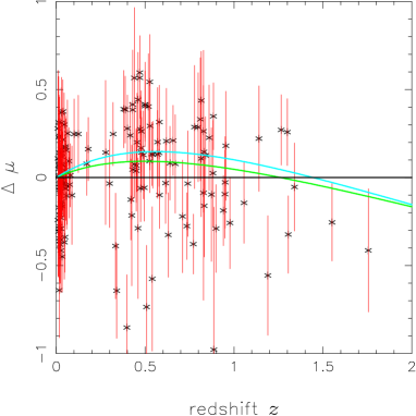
Figure 5: The green curve is the Hubble plot for the best fit model with $p/r=0.385$, $s=0.66$ and $H_{0}=64.0$. For comparison we also show the best fit $\Lambda CDM$ model (blue curve).

Accepting the values of the parameters obtained from fit we can now estimate various properties of the universe and compare with known values. Since best fit $p/r=0.385,s=0.66,H_{0}=64.0$ and we argued $p=1$, it follows, $r=2.6$ and $\alpha=0.46H_{0}$ . Thus the age of the universe according to this model is $t_{0}=\log({r})/{2\alpha}=15.2$ Gyr. Also $(\Omega_{DM})_{0}=0.39,(\Omega_{DE})_{0}=0.61$, $q_{0}=p/rs-1=-0.42$. These values are close to the currently accepted values. The deceleration parameter and redshift in this model are related by

$$q(z)=\frac{0.58}{0.615(1+z)^{-1.5}+0.385}-1\,\,,$$ (28)

and is found to represent an universe which is accelerating at present epoch but was decelerating in remote past (see fig (6)). This fact is also in agreement with current picture. The transition takes place at $z=1.15$. Note also that apart from the best–fit values there are a whole range of values of the parameters which are allowed at different confidence levels.

Figure 6: The deceleration parameter calculated for the best fit model as in previous figure. We see that the universe starts decelerating around $z\sim 1$.

It is obvious that there are many inadequacies in this model. For instance in the remote past there should be a radiation–dominated phase and the amount of radiation should decay to very small values in the present epoch. At best, this model can accomodate the late–time accelerated phase which, by and large, has been our goal. We have an analytic expression for the scale factor and the tachyon field. In addition, we have made a simplistic assumption about dark matter and dark energy being born out of the same scalar field. In some sense, our model tests how good this assumption is. The fact that the model fits the data quite well is appealing but to improve on it we must add further necessary features which are required for a realistic cosmological model. Finally, it might be worthwhile looking at cosmological perturbations in this model and try to use WMAP data to set more stringent bounds on the parameters tegmark03 ; WMAP .

- (1) A. G. Riess et al, Astron. J. 116, 1009 (1998) [ArXiv: astro-ph/9805201]; A. V. Filippenko, A. G. Riess, Phys. Rept. 307, 31-44 (1998) [ArXiv: astro-ph/9807008]
- (2) V. Balasubramanian, Class.Quant.Grav. 21, S1337 (2004) [ArXiv: hep-th/0404075]; E. S. Santini, G. A. Lemarchand [ArXiv: astro-ph/0410056]; R. Wigmans, [ArXiv: astro-ph/0409033]; A. B. Balakin, Gen.Rel.Grav. 36, 1513 (2004) [ArXiv: gr-qc/0409024]; S. Ray, U. Mukhopadhyay [ArXiv: astro-ph/0407295]
- (3) C. Armendariz-Picon, V. Mukhanov, P. J. Steinhardt, Phys.Rev.Lett. 85, 4438 (2000), [ArXiv: astro-ph/0004134 ]; V. Sahni, A. Starobinsky, Int.J.Mod.Phys. D9 373-444 (2000); P. J. E. Peebles, B. Ratra, Rev.Mod.Phys. 75, 559 (2003) [Arxiv: astro-ph/0207347]; T. Padmanabhan, Curr. Sci.88, 1057 (2005)
- (4) I. Maor, R. Brustein, Phys.Rev. D67, 103508 (2003) [ArXiv: hep-ph/0209203]; V. H. Cardenas, S. D. Campo, Phys.Rev. D69, 083508 (2004), [ArXiv: astro-ph/0401031]; P. G. Ferreira, M. Joyce, Phys. Rev. D58, 023503
- (5) R. R. Caldwell, M. Kamionkowski, N. N. Weinberg, Phys.Rev.Lett. 91, 071301 (2003) [ArXiv: astro-ph/0302506]; V. B. Johri, Phys.Rev. D70 041303 (2004), [ArXiv: astro-ph/0311293]; V. Sahni, [ArXiv: astro-ph/0403324]; S. Nojiri and S. D. Odintsov, Phys. Letts. B562,147 (2003); S. Nojiri and S. D. Odintsov, Phys. Lett. B571 (2003) 1
- (6) A. Sen, ArXiv: hep-th/0410103
- (7) A. A. Tseytlin, String cosmology and dilaton, in String quantum gravity and physics at the Planck scale, Erice, 21-28 June 1992, ed. N. Sanchez, World Scientific, 1993, [ArXiv: hep-th/9206067]; J. E. Lidsey, D. Wands, E. J. Copeland, Superstring Cosmology, Phys.Rept. 337, 343-492 (2000) [ArXiv: hep-th/9909061]
- (8) G. W. Gibbons, Phys.Lett. B537 1 (2002) [ArXiv:hep-th/0204008]; G. W. Gibbons, Class.Quant.Grav. 20, S321 (2003) [ArXiv: hep-th/0301117]; P. F. Gonzalez-Diaz, [ArXiv: hep-th/0408225]; B. C. Paul, M. Sami, Phys.Rev. D70, 027301 (2004) [ArXiv: hep-th/0312081] M. Fairbairn, M. H.G. Tytgat, Phys.Lett. B546, 1 (2002) [ArXiv: hep-th/0204070]; G. Calcagni, Phys.Rev. D69, 103508 (2004), [ArXiv: hep-ph/0402126]; G. Felder, L. Kofman, A. Starobinsky, JHEP 0209, 026 (2002) [ArXiv: hep-th/0208019]; A. Mazumdar, S. Panda, A. Pérez-Lorenzana, Nucl.Phys. B614, 101 (2001) [ArXiv:hep-ph/0107058]; X. Li, D. Liu, J. Hao, [ArXiv: hep-th/0207146]
- (9) A. Sen, JHEP 0207 065 (2002) [ArXiv:eprint hep-th/0203265]
- (10) T. Padmanabhan and T. Roy Choudhury, Phys.Rev. D66 081301 (2002) [ArXiv: hep-th/0205055 ]
- (11) T.Padmanabhan, Phys.Rev. D66, 021301 (2002), [ArXiv: hep-th/0204150]; J. S. Bagla, H. K. Jassal, T. Padmanabhan, Phys.Rev. D67, 063504 (2003) [ArXiv: astro-ph/0212198],
- (12) C. Kim, H. B. Kim, Y. Kim, Phys.Lett. B552 111 (2003) [ArXiv: hep-th/0210101];
- (13) D. A. Steer, F. Verizzi, Phys.Rev. D70 043527 (2004) [ArXiv: hep-th/0310139]
- (14) A. Feinstein, Phys. Rev. D66, 063511 (2002)
- (15) M. Sami, P. Chingangbam, T. Qureshi, Phys.Rev. D66 043530 (2002) [ArXiv: hep-th/0205179]
- (16) A. G. Riess et. al., Astrophys. J. 607, 665 (2004)
- (17) M. Tegmark, et al., Phys.Rev. D69, 103501 (2004)
- (18) H.K.Jassal, J.S.Bagla, T. Padmanabhan, Mon.Not.Roy.Astron.Soc.Letters, 356, L11 (2005) [astro-ph/0404378]