Tracing large-scale structure at high redshift with Lyman-$\alpha$ emitters: the effect of peculiar velocities

We investigate the effect of peculiar velocities on the redshift space distribution of $z\ga 2$ galaxies, and we focus in particular on Ly$\alpha$ emitters. We generate catalogues of dark matter (DM) halos and identify emitters with halos of the same co-moving space density ($M(Ly{\alpha}\ emitters)\approx 3\times 10^{11}\hbox{${\rm M}_{\odot}$}$). We decompose the peculiar velocity field of halos into streaming, gradient and random components, and compute and analyse these as a function of scale. Streaming velocities are determined by fluctuations on very large scales, strongly affected by sample variance, but have a modest impact on the interpretation of observations. Gradient velocities are the most important as they distort structures in redshift space, changing the thickness and orientation of sheets and filaments. Random velocities are typically below or of the same order as the typical observational uncertainty on the redshift. We discuss the importance of these effects for the interpretation of data on the large-scale structure as traced by Ly$\alpha$ emitters (or similar kinds of astrophysical high-redshift objects), focusing on the induced errors in the viewing angles of filaments. We compare our predictions of velocity patterns for Ly$\alpha$ emitters to observations and find that redshift clumping of Ly$\alpha$ emitters, as reported for instance in the fields of high-redshift radio galaxies, does not allow to infer whether an observed field is sampling an early galaxy overdensity.

1 Introduction

It has become feasible to obtain accurate redshifts for large samples of distant objects and produce 3-dimensional maps of the universe out to redshifts 3 and beyond. This has allowed quantitative studies of the large-scale structure of the distant Universe using Lyman-Break Galaxies (LBGs, see, e.g., Adelberger et al. 1998; Miley et al. 2004), Ly$\alpha$ emitters (Warren & Møller 1996; Steidel et al. 2000; Møller & Fynbo 2001; Fynbo, Møller & Thomsen 2001; Shimasaku et al. 2003), extremely red objects (Daddi et al. 2003), or radio galaxies (Pentericci et al. 2000; Venemans et al. 2002) as tracers. These surveys are consistent with the galaxies tracing the characteristic filamentary pattern, aptly called the ‘cosmic web’  in the dark matter, a generic feature of structure formation in a cold dark matter dominated universe.

In such 3D maps the third dimension is given by redshift and therefore they are deformed by the peculiar velocities of the galaxies. For example, infall onto clusters introduces a characteristic ‘finger of god’ pattern in the CfA redshift survey (Huchra et al., 1983). The peculiar velocities can be thought of as the sum of three components $(i)$ a streaming flow (driven by fluctuations on very large scales), $(ii)$ a coherent component that distorts the large-scale structure and $(iii)$ a small-scale noise term due to highly non-linear motions. Peculiar motions may change the apparent inclination angle at which filaments are observed, so if one wishes to apply an Alcock-Paczyński test on the distribution of inclination angles of filaments (Alcock & Paczyński 1979; Møller & Fynbo 2001), then it is imperative to understand at which scales such an analysis will not be systematically biased (Weidinger et al. 2002). Peculiar motions may also lead to an apparent enhancement in the clumpiness of the redshift distribution of Ly$\alpha$ emitters in deep narrow-band observations, as we will show below.

In this paper we follow Haehnelt, Natarajan & Rees (1998) and identify Ly$\alpha$ emitters with halos in our DM simulations by requiring that the halos of the corresponding mass have the same number density as the Ly$\alpha$ emitters. Such a simple biasing scheme should work well if the duty cycle of Ly$\alpha$ emission is close to one. We then investigate to what extent peculiar velocities influence the observed distribution of Ly$\alpha$ emitters. Although we focus on the large-scale structure as traced by Ly$\alpha$ emitters, our conclusions can be applied to other classes of objects as well.

This paper is organised as follows. In Sect. 2 we decompose the velocity field of DM halos into streaming, gradient and random components, and show how to estimate such velocity components on DM halo catalogues generated with the pinocchio code (Monaco et al. 2002). In Sect. 3 we quantify the velocity components and give analytic fits to reproduce the results. The observational consequences of these results on the reconstruction of viewing angles of filaments and on the redshift distribution of Ly$\alpha$ emitters in narrow band imaging selected volumes at high redshift are given in Section 4. Section 5 concludes. More details on the extension of the pinocchio code to multi-scale runs and on the connection between DM halos and observed astrophysical objects are given in three appendices.

In this paper we assume a scale invariant, vacuum energy dominated flat universe with parameters $(\Omega_{m},\Omega_{\Lambda},n,h,\sigma_{8})=(0.3,0.7,1,0.7,0.9)$ (e.g. Spergel et al. 2003), where the symbols have their usual meaning.

2 Quantification of peculiar velocity components

Consider a set of DM halos in a given volume; the (highly correlated) peculiar velocity field traced by these halos can be decomposed in three components that have different effects on observations in the redshift space (e.g. Weidinger et al. 2002): (i) the mean velocity of the set, or streaming velocity, (ii) a gradient component of velocities along the volume and (iii) the residual (random) component. Performing a Taylor expansion of the peculiar velocity around the set’s mean velocity, these components are:

$${\bf x} = {\bf r}/a$$

$${\bf v}({\bf x}) \equiv a{d{\bf x}\over dt}$$ (1)

$$= {\bf v}({\bf x}_{0})+\left[({\bf x}-{\bf x}_{0})\cdot\nabla_{\bf x}\right]{\bf v}\,({\bf x}_{0})+{\bf v}_{r}({\bf x}).$$

Here, $a$ is the scale factor, $\bf{x}$ is the co-moving position of the halo, and the peculiar velocity ${\bf v}$ at position $\bf{x}$ is written as a sum of a streaming, gradient and random component. The geometrical meaning of the three terms is straighforward: the streaming velocity gives the bulk motion of the whole set; the gradient component is responsible for distortions of the redshift-space patterns and can change the shape of the structure traced by the set; random velocities are considered here as a noise. Note that the gradient component is a tensor, but we will restrict ourselves to the diagonal components:

$$h_{i}=\partial v_{i}/\partial x_{i}\,.$$ (2)

These velocity components are of course only defined once the volume containing the set has been identified, i.e. once a (co-moving) scale has been chosen. In other words, these quantities are scale-dependent.

2.1 Velocity components in linear theory

Figure 1: Predictions of linear theory for the three velocity statistics. Left panel: streaming and random velocities (equations 7 and 6). Right panel: gradient velocity (equation 9).

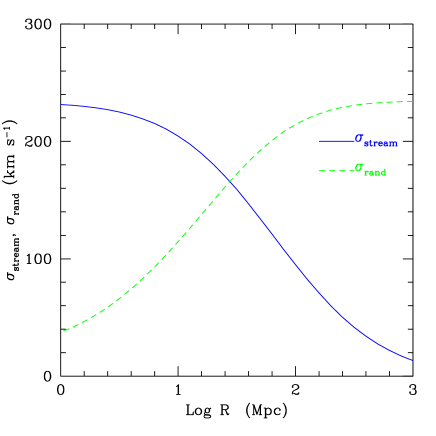
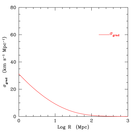
It is useful to consider the predictions of linear theory for the three velocities defined above (equation 1) as a function of scale, both to have an idea of their behaviour and as a basis for constructing analytic fits of the simulation results in the next section (see also Hamana et al. 2003).

In the Zel’dovich (1970) approximation, the peculiar velocity ${\bf v}$ of a halo is related to the gravitational potential $\phi$ by (e.g. Peebles 1980)

$${\bf v}=-a(t)\dot{D}(t)\nabla\phi\,\,,$$ (3)

where a dot denotes a time derivative. In turn, $\phi$ is related to the underlying density field $\delta({\bf x},t)\equiv\rho({\bf x},t)/\langle\rho({\bf x},t)\rangle$ through Poisson’s equation,

$$\nabla^{2}\phi({\bf x},t)={1\over a}\,\delta({\bf x},t)\,.$$ (4)

In these equations $D(t)$ is the growing mode of the density perturbation. If $P(k)$ denotes the power spectrum of density fluctuations, then Poisson’s equation combined with equation (3) shows that the spectrum of velocity perturbations is $P_{v}\propto k^{-2}\,P(k)$. Therefore the (1D) variance of the peculiar velocity in linear theory is

$$\sigma^{2}_{v}=\frac{1}{3}(a\dot{D})^{2}\frac{1}{2\pi^{2}}\int_{0}^{\infty}P(k)dk\,.$$ (5)

Note that $\sigma^{2}_{v}$ converges readily on small scales where $P(k)\propto k^{n}$ with $n\sim-2$ to $-3$, but converges only slowly on large scales, as is well known.

We now focus on a system of size $R$ to decompose $\sigma^{2}_{v}$ in terms of a streaming, gradient, and random component. The variance of the streaming velocity of the matter in the volume $V$ can be computed by smoothing $\phi$ with a window function $W_{R}({\bf q})$ (with $V\sim R^{3}$). If $\tilde{W}$ denotes the Fourier transform of $W$, then

$$\sigma^{2}_{\rm stream}(R) = \frac{1}{3}(a\dot{D})^{2}\sigma^{2}_{0}(R)$$ (6)

$$\sigma^{2}_{\rm rand}(R) = \sigma^{2}_{v}-\sigma^{2}_{\rm stream}(R),$$ (7)

where

$$\sigma^{2}_{l}(R)\equiv\frac{1}{2\pi^{2}}\int_{0}^{\infty}k^{l}\,P(k)\tilde{W}^{2}(kR)dk\,.$$ (8)

Similarly, the rms gradient

$$\sigma^{2}_{\rm grad}(R)=\frac{1}{3}(a\dot{D})^{2}\,\sigma^{2}_{2}(R)\,.$$ (9)

Note that $\sigma^{2}_{2}(R)$ in this equations is also the mass variance on scale $R$. In the following we will use a top-hat filter, so that the mass variance will be related to spherical volumes of radius $R$.

In Fig. 1 we plot the streaming, gradient and random components predicted by linear theory at $z=2$ as a function of scale $R$. Streaming velocities dominate on scales smaller than $\sim 30$ Mpc; on larger scales random velocities dominate. The cross-over scale is a measure of the velocity correlation in linear theory, and is similar to the size of the largest observable structure (filament or void) at the given redshift. The rms gradient $\sigma_{\rm grad}(R)$ is usually a small fraction of the Hubble constant $H(z)$.

In the next section we compute these variances using simulations.

2.2 Simulations

As we saw in the previous section, peculiar velocity fields are correlated over large scales, hence simulations need to be performed in a large volume to adequately sample the large-scale modes. Combined with the need to be able to resolve small halos, we require simulations with a large dynamic range. Furthermore, to test convergence of results and decrease sample variance we need to run many simulations. The pinocchio algorithm (Monaco et al. 2002a; Monaco, Theuns & Taffoni 2002b; Taffoni, Monaco & Theuns 2002) is ideally suited for this purpose.

pinocchio uses Lagrangian perturbation theory and an algorithm to mimic the hierarchical build-up of DM halos to predict the masses, positions and velocities of dark matter halos as a function of time. The agreement between pinocchio and a full scale $N$-body simulation is very good, even when comparing the properties of individual halos. pinocchio does not compute the density profile of the halos, and as a consequence is many orders of magnitude faster than an $N$-body simulation. A simulation with 256³ particles requires a few hours on a PC.

As we will show below, a typical Ly$\alpha$ emitter lies in a halo of mass $\sim 3\times 10^{11}\hbox{${\rm M}_{\odot}$}$, so if we want to resolve a halo with 150 particles, then the particle mass is $2\times 10^{9}\hbox{${\rm M}_{\odot}$}$. In a simulation with $256^{3}$ particles, and given our assumed cosmology, this limits our box size to $\sim 65\,h^{-1}\hbox{\rm Mpc}$, too small to properly sample the large-scale velocity field. Fortunately it not necessary to perform much larger, computationally expensive simulations, because it is straightforward to add long-wavelength perturbations to pinocchio. This is explained in Appendix A, while Appendix B quantifies the accuracy of pinocchio in reproducing the velocity components defined above.

To address convergence of peculiar velocities and sample variance, we have run many realisations (Table 1). For the reference cosmology, we have performed 10 standard pinocchio  runs with a single grid of size $L=65\,h^{-1}$ Mpc and grid spacing $\Delta$ such that $L/\Delta=256$ ($\Delta=0.254\,h^{-1}$ Mpc), and 11 pinocchio  runs with two grids, using a high-resolution grid with $L_{2}=65\,h^{-1}$, $L_{2}/\Delta_{2}=256$, and a low-resolution with $L_{1}=8L_{2}=520\,h^{-1}$ Mpc, $L_{1}/\Delta_{1}=64$ ($\Delta=8.125\,h^{-1}$ Mpc).

Table 1: pinocchio  runs performed, the particle mass is $6.7\times 10^{8}$. $L_{1}$ and $\Delta_{1}$ ($L_{2}$ and $\Delta_{2}$) are the size of the low (high) resolution box and grid spacing, respectively. Runs of given type only differ in the random seed.

run id	# of runs	$L_{1}$	$L_{1}/\Delta_{1}$	$L_{2}$	$L_{2}/\Delta_{2}$
		$h^{-1}\hbox{\rm Mpc}$		$h^{-1}\hbox{\rm Mpc}$
P1	10	-	-	65	256
P2	11	520	64	65	256

2.3 Computing velocity statistics from halo catalogues

Figure 2: Velocity statistics for halos with mass $M>10^{11}$ M_⊙ at $z=2$ in the pinocchio  simulations of Table 1. Thick lines and thin lines denote the mean and 1-$\sigma$ dispersion of these statistics respectively, for runs P1 (dashed) and P2 (full lines). Note how the P1 simulation severely underestimates the streaming velocity because of the missing large-scale power in the small simulation box.

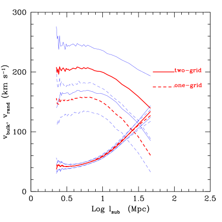
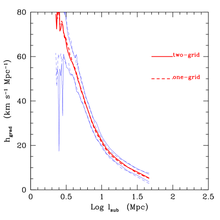
To compute streaming, gradient and random velocities from the pinocchio runs, we have subdivided the simulated boxes into $n^{3}$ cubic sub-boxes of side $l_{\rm sub}=l_{\rm box}/n$, where $n$ is a running integer. For each subdivision $n$, each sub-box $(j,n)$ (where $j=[0,n^{3}]$) is centred on ${\bf x}_{0,j,n}$ and contains $N_{j,n}$ dark matter halos more massive than a given threshold mass. For each sub-box $(j,n)$ and for each spatial component $i$ we compute the streaming and gradient velocities as the zero point and slope of a linear regression with respect to position $x_{i}$ of the velocities $v_{i}$ of all the halos:

$$v_{i}({\bf x}_{0,j,n})=\frac{\sum x_{i}^{2}\sum v_{i}-\sum x_{i}\sum x_{i}v_{i}}{N_{j,n}\sum x_{i}^{2}-(\sum x_{i})^{2}}$$ (10)

$$\frac{\partial v_{i}}{\partial x_{i}}({\bf x}_{0,j,n})=\frac{N_{j,n}\sum x_{i}v_{i}-\sum x_{i}\sum v_{i}}{N_{j,n}\sum x_{i}^{2}-(\sum x_{i})^{2}}$$ (11)

The sum is over the $N_{j,n}$ halos in the sub-box $(j,n)$. Random velocities are computed as the residuals of velocities with respect to the linear regression. For each sub-box $(j,n)$ and for each component $i$ we compute the variance of these residuals:

$$\sigma_{r,i}^{2}({\bf x}_{0,j,n})=$$

$${\rm var}\left(v_{i}({\bf x})-v_{i}({\bf x}_{0,j,n})-({\bf x}-{\bf x}_{0,j,n})_{i}\frac{\partial v_{i}}{\partial{x_{i}}}({\bf x}_{0,j,n})\right)$$

Finally, for each sub-box size $n$ we compute the variance of these quantities over all sub-boxes $j$ that contain at least 5 objects ($N_{j,n}\geq 5$), and express the result as a function of the sub-box length $l_{\rm sub}$:

$$v_{{\rm stream},i}^{2}(l_{\rm sub}) = \left\langle\left(v_{i}({\bf x}_{0,j,n})\right)^{2}\right\rangle_{j}$$

$$h_{{\rm grad},i}^{2}(l_{\rm sub}) = \left\langle\left(\frac{\partial v_{i}}{\partial x_{i}}({\bf x}_{0,j,n})\right)^{2}\right\rangle_{j}$$ (13)

$$v_{{\rm rand},i}^{2}(l_{\rm sub}) = \left\langle\sigma^{2}_{r,i}({\bf x}_{0,j,n})\right\rangle_{j}$$

Notice that the second quantity, $h_{{\rm grad},i}$, has the same dimension as the Hubble constant, while the other two are pure velocities. In the following, where not otherwise stated, we will show for the three velocity statistics the average over the three directions.

3 Results

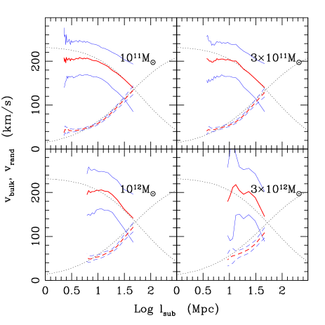
Fig. 2 shows the streaming, gradient and random velocity variances for halos larger than $10^{11}$ M_⊙ at $z=2$, as a function of scale averaged over the P1 simulations (dashed lines). As for linear theory, on small scales streaming flows dominate and random velocities are relatively small, while the reverse is true at larger scales. However, the relatively modest value of the streaming velocity is mostly an artifact connected to the small box size and the resulting poor sampling of the large scale modes; in a low-density universe velocity fields are highly correlated, and to achieve convergence for the streaming velocity it is necessary to average over volumes as large as several hundred Mpc. Fig. 1 shows that the expected streaming flow velocity drops below 50 km s^-1 only at scales of $\sim$200 Mpc. The P2 simulations do not suffer from lack of large scale power, and the streaming velocities are much larger (Fig. 2). Note that the random and gradient dispersions are similar in the smaller boxes.

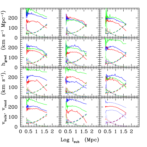
Due to the large correlation length of the velocity field, the three velocity statistics (especially the streaming motions) show a great deal of variation among different realisations, which we call sample variance. Fig. 3 shows the random and streaming velocities for each of the P2 runs separately. Notice that the P1 realisations artificially suppress some of the sample variance by imposing periodic boundary conditions, while the P2 realisations do not have this drawback. Here we show in each panel the streaming, gradient and random velocities as computed in the three directions. The curves fluctuate much from one realisation to the other. The 12th panel shows the average with 1$\sigma$ fluctuations, the same quantity shown in Fig. 2.

This figure shows clearly the importance of a proper quantification of sample variance. This is important not only to test the reliability of the predictions, but also to quantify the interval in which observed data are expected.

Figure 3: Sample variance of velocity statistics for the 11 runs of the P2 simulation. Continuous, dotted and dashed lines denote streaming, gradient and random velocity variances, respectively. Here we show the three spatial components separately. The 12th panel contains the average variance for all runs, with the corresponding 1-$\sigma$ dispersion.

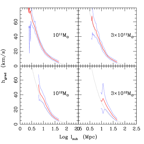
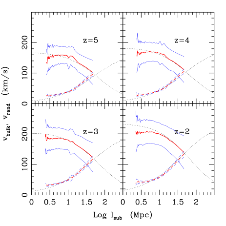
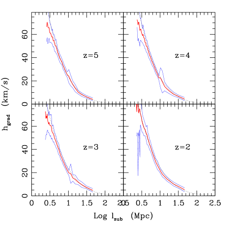
The velocity statistics shown above depend on DM halo mass, redshift and cosmology. Figs. 4 and 5 illustrate the mass and redshift dependence. In the same figures we show analytic fits, based on linear theory, to the velocity statistics. In particular, streaming velocities are reasonably well fit on the scales of interest by the simple linear theory prediction of equation 7. A weak mass dependence is noticeable, however it is much stronger for gradient and random velocities. Such a mass dependence is expected since halos are biased tracers of the mass (see also Hamana et al. 2003).

Because of the self-similar character of gravity, we expect to be able to fit the mass-dependence by a simple function of the spectral moments $\sigma_{l}$ (equation 8). The mass of the halo depends on $\sigma_{2}(R)$, while the velocity variances depend on $\sigma_{0}(R)$ (equations 6 and 7). The (top-hat) co-moving smoothing radius $R$ is connected to the halo mass $M$ through the relation $4\pi R^{3}\rho_{0}=M$, where $\rho_{0}$ is the actual average matter density. With this $M-R$ relation the mass variance relative to $M$, $D(z)\sigma(M)$ is then computed. The mass dependence of random and gradient velocities is then reasonably well reproduced (Fig. 4, 5) by

$$h_{\rm grad,fit}(R)=\frac{1}{\sqrt{3}}(a\dot{D})\sigma_{2}(R)\left(1+0.8\frac{\sigma}{D(z)\sigma_{2}(R)}\right)$$ (14)

$$v_{\rm rand,fit}(R)=\frac{1}{\sqrt{3}}(a\dot{D})\sigma_{0}(R)\left[1+\left(\frac{\sigma}{D(z)\sigma_{2}(R)}\right)^{0.5}\right]^{-1}$$ (15)

where $4\pi R^{3}\rho_{0}=M$. They give acceptable fits at scales larger than 10 co-moving Mpc, although some residual mass dependence is present; in particular, more massive objects are not perfectly reproduced.

We have verified that the dependence on cosmological parameters is correctly reproduced by these fits by performing additional pinocchio  simulations, using the same random seeds to be less affected by sample variance.

Figure 4: Velocity statistics for different halo masses at $z=2$. The average and variance for the simulation P2 are shown. Dotted lines give the analytic fits (equations 7, 14 and 15).

Figure 5: Same as Fig. 4 but for $M>10^{11}$ M_⊙ and different redshifts.

4 Observational consequences

In the previous sections we characterised the effect of peculiar velocities on the distribution of halos in redshift space. To apply this result to galaxies we need to known how to associate galaxies with dark matter halos. In this section we apply a very simple biasing scheme where we associate galaxies of a given type with halos with the same co-moving space density. More complex schemes have appeared in the literature (e.g. based on the halo occupation distribution, Berlind et al. 2003) but our model has the advantage of simplicity and it is sufficient for our purpose.

Ly$\alpha$ emitters are the most numerous emission selected objects known at high redshifts, suggesting that they must inhabit relatively low-mass halos. In a deep search in two fields at z=2.85 and z=3.15, Fynbo et al. (2003) determined the co-moving space density $n_{Ly\alpha}$ of spectroscopically confirmed Ly$\alpha$ emitters down to their Ly$\alpha$ flux detection limit of $7\times 10^{-18}$ erg s^-1 cm^-2 to be $\log(n_{Ly\alpha})=-2.6$. Assuming that 100% of DM halos host a Ly$\alpha$ emitter, the measured space density in our cosmology is typical of halos of mass $6\times 10^{11}$ M_⊙. The duty cycle could be lower than 100%; for LBGs, only 25% show significant Ly$\alpha$ emission (e.g., Shapley et al. 2003). However, this is likely to be a lower limit to the duty cycle of typical Ly$\alpha$ emitters, that have smaller star formation rates and then are less affected by dust obscuration. If a 25% duty cycle is adopted, the corresponding halo mass decreases to $2\times 10^{11}$ M_⊙ . These numbers should bracket the solution, and justify the choice of $\sim 3\times 10^{11}$ M_⊙ anticipated in Section 2.2.

4.1 The influence of velocities on Ly$\alpha$ filaments

Several properties combine to make Ly$\alpha$ emitters a good tracer for mapping large-scale structure. Because they have higher space density than any other class of detectable objects at high redshifts they provide the best possible sampling of structures at all scales, their redshift is always measured from the same emission feature so redshifts are obtained in a very homogeneous way, and their low masses make them weakly biased tracers of the large-scale structure. A natural prediction of hierarchical clustering is then the likely detection of filaments and pancakes in the 3D distribution of Ly$\alpha$ emitters. One such filament traced by Ly$\alpha$ emitters has been detected at $z=3.04$ (Møller & Fynbo 2001), but the inferred 3D properties of filaments will be modified by peculiar velocities and to recover their true properties it is necessary to understand those effects that can be divided into three distinct components.

The streaming velocity of galaxies on the observed scale of the filament will change the mean redshift by a small amount, $\sim 150$ km s^-1 on scales of tens of Mpc, amounting to a negligible shift in redshift of $5\times 10^{-4}$. The gradient component will distort the viewing angle of the filament; in particular the relative (systematic) error on the line-of-sight dimension of the filament will be:

$$\epsilon=\frac{\frac{\delta v}{\delta x}(1+z)}{H(z)}$$ (16)

(The gradient is multiplied by $(1+z)$ because the Hubble constant is defined in terms of physical distance, in place of co-moving). At that scale the gradient will be of about 10 km $s^{-1}$ Mpc^-1, and the relative error will be 0.13 (for a Hubble constant of 312 km $s^{-1}$ Mpc^-1, which is the Hubble constant at $z=3$ in the assumed cosmology). This will also be the relative error of the arc cosine of the viewing angle. The corresponding systematic error on the inclination angle will hence typically be about 2-3^o, which is similar to the 1.9^o error due to sparse sampling on the inclination angle of the $z=3.04$ filament (Weidinger et al. 2002).

Random velocities will thicken the filament. For our test case, velocities just above 100 km s^-1 are expected, so they will contribute in a similar way as the typical uncertainty in the redshift.

These effects should be taken into account when estimating, for instance, the cosmological parameters by applying the extended Alcock-Paczyński test on the distribution of viewing angles (Møller & Fynbo 2001; Weidinger et al. 2002).

4.2 Enhancement of clustering in redshift space

The power of the approach presented here goes beyond a statistical quantification of the effects of the velocity components. We illustrate this point by giving an example of interpretation of data based on simulated catalogues of Ly$\alpha$ emitters.

Fynbo et al. (2003) detected a significant degree of redshift clumping in the field around a DLA toward the quasar Q2138-4427 (at $z=2.85$). This is clearly visible in their Fig. 8, where redshifts clump into a limited interval, much narrower than the redshift-depth corresponding to the filter. In the other field of that study (Q1346-0322 at $z=3.15$), the redshifts are uniformly distributed over the range defined by the filter. The clumping can be quantified by $\sigma_{z}$, the root-mean-square of the redshift distribution, found to be 0.018 (with 19 emitters) and 0.006 (with 23 emitters) for the fields of Q1346-0322 and Q2138-4427 respectively. These $\sigma_{z}$ values should be compared to the expected value of 0.019 based on a simple Monte Carlo simulation using the filter transmission as selection function. Hence, the Q2138-4427 field clearly shows a significant degree of structure. Similar redshift clumping has been reported in the fields of two radio galaxies at redshifts $z=2.14$ and $z=4.10$ (Pentericci et al. 2000; Venemans et al. 2002).

It is interesting to ask how often and under what conditions does similar redshift clumping occur in the simulations? Peculiar velocities can influence the clumping of redshifts in different ways. While streaming flows shift the whole redshift distribution, gradient velocities can increase or decrease the dispersion $\sigma_{z}$. If a mildly non-linear structure (a filament or a pancake) is present in the field, it is known that the peculiar velocity field (its gradient component, in our terminology) will tend to flatten it, thus decreasing $\sigma_{z}$ (see, e.g., Strauss & Willick 1995). Random velocities will instead tend to increase $\sigma_{z}$.

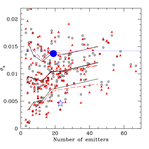
To assess the likelihood of the observed $\sigma_{z}$ values and the influence of peculiar velocities we extract 15 mock catalogues from each of the P2 runs. Each mock catalogue is extracted by picking random redshift-space volumes with sizes corresponding to the volume sampled by the observation and selecting all DM halos more massive than $3\times 10^{11}$ M_⊙ contained in the volume. The connection between minimal Ly$\alpha$ flux and minimal halo mass is fixed loosely (see Sect. 4.1-4.3), so the number of emitters here is to be considered as indicative. However, as long as such small halos trace the same structure nearly independently of mass, $\sigma_{z}$ should not be affected by this assumption. Referring to a filter FWHM of 60 Å and a field of view of 6.7 arcmin, we extract volumes of 12.4 $\times$ 12.4 $\times$ 47.0 co-moving Mpc (the line of sight corresponding to the longer dimension). Boxes are required to contain at least three objects. Redshifts are computed along the major axis of the extracted volume. Fig. 6 shows the resulting $\sigma_{z}$ of the redshift distributions of the mock catalogues as a function of the number of mock emitters found in the box which is a measure of overdensity. The $\sigma_{z}$ values are computed both neglecting and considering peculiar velocities. The lines show the average and $\pm$1-$\sigma$ intervals of the $\sigma_{z}$ distribution. The expected $\sigma_{z}$ value in the case of no clumping is 0.0142; due to the well-known clustering of halos, significantly lower values are expected on average.

The observational points are reported as well. As the filters are more similar to Gaussians than to top-hats, the expected $\sigma_{z}$ value for a uniform distribution (0.019) is higher than in our case which assumed a top-hat (0.014), therefore we multiply the observed values by $0.014/0.019=0.737$.

As it is apparent, peculiar velocities are responsible for decreasing the value of $\sigma_{z}$ by some 10% when it is already small; these are cases of filaments (or pancakes) seen perpendicularly to the line of sight, where the effect of flattening by peculiar velocities is largest. The two observed points are well within the predicted range, so these fields are by no means rare cases. In particular, the low value of $\sigma_{z}$ in the Q2138-4427 field, coupled to the moderately high value of the overdensity inferred, can be interpreted, as mentioned above, as the effect of a flattened structure. It is a 1.76$\sigma$ event so equally low values of $\sigma_{z}$ will be expected in 4.5% of all observed fields. If peculiar velocities are neglected, the Q2138-4427 field turns out to be a 1.93$\sigma$ event, only marginally rarer.

Pentericci et al. (2000) and Venemans et al. (2002) both use the observed redshift clumping to argue for substantial overdensities around radio galaxies, and claim these suggest the detection of a protocluster. They assume that the overdensity $\delta$ can be estimated from

$$\delta=\frac{n_{obs}\times\mathrm{fwhm}_{\mathrm{filter}}}{n_{field}\times\mathrm{fwhm}_{z}},$$ (17)

where $n_{obs}$ is the observed number density in the field containing the radio galaxy, $n_{field}$ is an estimate of the number density of a reference field and $\mathrm{fwhm}_{\mathrm{filter}}$ and $\mathrm{fwhm}_{z}$ are the full-width-at-half-maxima of the filter transmission (transformed to redshift space) and the observed redshift distribution, respectively. However, as seen from Fig. 6 $\sigma_{z}$ is not a decreasing function of density. In fact, it is more likely to have a low $\sigma_{z}$ in the redshift distribution in a field with few Ly$\alpha$ emitters than in an overdense field. Therefore, the only valid way of resolving whether radio galaxies are located in protoclusters is to obtain an accurate measurement of the number density of galaxies in blank fields at similar redshifts.

Figure 6: Redshift dispersion, $\sigma_{z}$, of Ly$\alpha$ emitters selected in a narrow-band field as function of the number of emitters. A big filled circle and a big star denote the fields around Q1346-0322 and Q2138-4427 (Fynbo et al. 2003), respectively. Filled triangles denote $\sigma_{z}$ in 165 mock samples of Ly$\alpha$ emitters, the mean and 1 sigma dispersion are indicated by thick and thin dashed lines respectively. In the mocks, Ly$\alpha$ emitters are assumed to reside in halos more massive than $3\times 10^{11}\hbox{${\rm M}_{\odot}$}$. Full lines and filled squares neglect peculiar velocities. The horizontal dotted line denotes the mean dispersion in the absence of peculiar velocities and clustering. Halo clustering decreases $\sigma_{z}$ significantly (dotted line compared to full line) but peculiar velocities do not have a strong effect (dashed line compared to full line). The observed points fall well within the range covered by the mocks.

5 Conclusions

We have characterised and quantified the effect of peculiar velocities in the reconstruction of large-scale structure at high redshift, with particular attention to Ly$\alpha$ emitters as tracers.

With the aid of pinocchio  simulations we have decomposed the velocity field of DM halos into a streaming flow, a gradient and a random velocity term, and computed them as functions of scale. The dependence of these velocity statistics on halo mass, redshift and cosmology has been quantified and fitting formulae have been proposed.

The main effects of these velocity components on the observational properties of Ly$\alpha$ emitters have been analysed. In particular, streaming flows are determined by fluctuations on very large scales, and are strongly affected by sample variance, but have a modest impact on the interpretation of observations. Gradient flows are mostly important, in that they influence the quantitative reconstruction of structures like the inclination angle of filaments, important for applying the extended Alcock-Paczyński test (Møller & Fynbo 2001), or the root-mean-square of the redshift distribution, important to recognise flattened structures (pancakes or filaments) perpendicular to the line of sight. Random velocities are typically below or of the same order as the observational uncertainty on the redshift.

The results presented here have been applied to quantify the influence of peculiar velocity on the reconstructed viewing angles of filaments at $z\simeq 3$. In particular, the effect of streaming velocities is negligible, gradient velocities give an error of 2-3^o degrees, similar but larger than the typical error due to sparse sampling, while random velocities add to the $\sim 100$ km s^-1 error on the redshift. Clearly, a proper quantification of such errors is necessary to implement an Alcock-Paczyński test to the inclination of filaments.

As a further example of the power of this approach, we have generated mock catalogues of Ly$\alpha$ emitters to assess the significance of a detected narrow distribution in redshift in a deep exposure. The observation is found to be a $\sim$2$\sigma$ event corresponding to a sheet of galaxies seen face on. Peculiar velocities give a modest but significant contribution to the narrowness of the redshift distribution, and this again corresponds to the dominant effect of gradient velocities with respect to random velocities. Moreover, we do not notice a significant anti-correlation between the abundance of emitters, a tracer of overdensity, and the degree of clumpiness, at variance with what is assumed by Pentericci et al. (2000) and Venemans et al. (2002).

The results presented here will be important for interpreting the upcoming data on the large-scale structure as traced by Ly$\alpha$ emitters. Further work will be aimed at generating mock catalogues of Ly$\alpha$ emitters that closely reproduce the observational selection effects, in order to devise tight observational tests for the hierarchical clustering model at $z\ga 2$.

Appendix A Adding long wavelength modes to pinocchio

Tormen and Bertschinger (1996) describe an algorithm to increase the dynamic range of a simulation by adding long-wavelength perturbations after the simulation has been done. However, as pointed out by Cole (1997), the algorithm neglects the coupling between long-wavelength linear modes and short-wavelength non-linear modes, and this strongly affects the clustering of halos. Fortunately, this is not a problem in pinocchio, since it is easy to correctly incorporate the effect of long wavelength modes on the non-linear collapse of structures. We begin by giving a very brief overview of the pinocchio algorithm, and then proceed to describe how one can easily add long wavelength modes.

The standard pinocchio algorithm operates on a realisation of a linear density field generated on a regular grid, identical to the grid used in the initial conditions of an $N$-body simulation. In a first step, a ‘collapse time’ is computed for each grid point (‘particle’) using a truncation of Lagrangian perturbation theory based on ellipsoidal collapse. The collapse time is the time at which the particle is deemed to fall into a high-density region (a halo or filament). In the second step, collapsed particles are gathered into halos, using an algorithm that mimics the hierarchical build-up of halos (see Monaco et al. 2002a for more details).

The calculation of the collapse times itself also involves two steps, (a) a series of linear operations on the initial density field, followed by (b) a non-linear calculation. For a Gaussian random field, the long- and short-wavelength perturbations are by definition independent, therefore it is trivial to perform the first step for long and short wavelengths separately. In contrast to the Tormen & Bertschinger (1996) implementation, the result of the calculation of the two step procedure (i.e. doing long and short wavelengths separately) gives identical result to doing the full calculation, yet requires significantly less computation.

The algorithm works as follows. Take the linear potential $\psi({\bf q})$, defined on the vertices ${\bf q}$ of a grid. The grid spacing $\Delta$, together with the extent of the grid, $L$, determine the range of waves that can be represented, namely between $2\Delta$ and $L$. However, consider now two grids, with spacings $\Delta_{1}$ and $\Delta_{2}$, and extents $L_{1}$ and $L_{2}$ respectively. Grid 2 represents a higher resolution grid contained within grid 1, and we want to add the long-wavelength perturbations of grid 1 onto grid 2, increasing the dynamic range from $L_{2}/\Delta_{2}$ to $L_{1}/\Delta_{2}$.

On the vertices of grid 2, we can add the contributions from fluctuations on grid 1 and grid 2 to obtain the potential $\psi$:

$$\psi({\bf q})=\psi_{1}({\bf q})+\psi_{2}({\bf q})\,,$$ (18)

Clearly $\psi$ has contributions from the full range of waves, $2\Delta_{2}$ to $L_{1}$. Of course the spacing of grid 1 is coarser than of grid 2, $\Delta_{1}>\Delta_{2}$, so equation (18) involves an interpolation from the coarser to the finer grid. But the key point is that, as long as the operations we are going to do on $\psi$ are linear, we can perform them on grids 1 and 2 independently, and just add the result at the end to compute the collapse time for the vertices of the higher resolution grid. The rest of the pinocchio  calculation now only applies to the high resolution grid, but we have to be aware of boundary effects on the edge of the smaller grid.

When initialising the Gaussian fluctuations on these grids, we use the power spectrum $P(k)\,\Theta(k_{1})$ on grid 1, and $P(k)\,(1-\Theta(k_{1}))\,\Theta(k_{2})$, where $P(k)$ is the desired linear power-spectrum, and the Heaviside function restricts the contribution from waves $>k_{1}$, respectively $k_{2}$. $k_{2}$ denotes the Nyquist frequency on the high-resolution grid, and $k_{1}$ should be smaller than the Nyquist frequency of the lower-resolution grid but larger than $2\pi/L_{2}$.

For the box and grid lengths given in Section 2.2 ($L_{2}=65\,h^{-1}$, $L_{2}/\Delta_{2}=256$, $L_{1}=8L_{2}=520\,h^{-1}$ Mpc, $L_{1}/\Delta_{1}=64$), we found that a good choice for $k_{1}=\pi/L_{1}$. The effective dynamic range of these simulations is thus $(L_{1}/\Delta_{2})^{3}=2048^{3}$, whereas the simulation time is more similar to performing two $256^{3}$ simulations. Given that the simulation time is dominated by the fast Fourier transforms on the grid that scale as $N\log(N)$, with $N=(L/\Delta)^{3}$, this is an acceleration of a factor of 352, and we effectively perform a $2048^{3}$ simulation in a few hours on a PC.

Figure 7: Velocity statistics comparing pinocchio  and $N$-body runs. Upper panels show the 100 Mpc/$h$ simulation of Monaco et al. (2002b) for $M>3\times 10^{11}$ M_⊙ at $z=2$, lower panels the 250 Mpc/$h$ simulation of Fontanot et al. (2003) for $M>3\times 10^{12}$ M_⊙ at $z=0$

Appendix B pinocchio accuracy in recovering peculiar velocity components

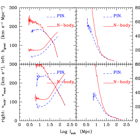
To check the accuracy achieved by pinocchio in predicting the three velocity statistics defined in Section 2.3 we compare the pinocchio result to those of two different $256^{3}$ N-body simulations, the 100Mpc/$h$ run used by Monaco et al. (2002b) and Taffoni et al. (2002), and the 250 Mpc/$h$ presented by Fontanot et al. (2003). In both cases we run pinocchio with a single grid, and on the same initial conditions as the simulations. The assumed cosmologies are similar to the reference one, except that $h=0.65$ in the first simulation, and $\sigma_{8}=0.8$ in the second one. For the first simulation, the mass resolution is a factor of 3 lower, so that $3\times 10^{11}$ M_⊙ halos are the smallest reliable ones. For the second simulation the mass of the particle is $\sim 10^{11}$ M_⊙, so that only halos with $M\ga 5\times 10^{12}$ M_⊙ are reliable. In order to have a sufficient number of halos, we test this simulation at $z=0$. Halos in both simulations have been selected with the usual friends-of-friends algorithm with a linking length 0.2 times the interparticle distance (Jenkins et al. 2001).

Fig. 7 shows the streaming, gradient and random velocity statistics for the PINOCCHIO and N-body runs. On scales larger than 10 co-moving Mpc at $z=2$ (or 20 at $z=0$) pinocchio systematically underestimates the random velocity by $\sim$30 km $s^{-1}$ while it reproduces fairly well the streaming velocity. The gradient component is underestimated at worst by $\sim$30%. At smaller scales these underestimates are larger, but the qualitative behaviour is always reproduced.

This level of agreement is expected, because pinocchio velocities are based on the Zel’dovich (1970) approximation, which is known to reproduce well the large-scale velocity field but to underestimate the small-scale, highly non-linear velocities. The latter are the result of infall of halos onto neighbours.

As the scales of interest are those relative to the large-scale structures observed (like filaments), roughly corresponding to the cross-over of streaming and random velocities, we conclude that pinocchio is sufficiently accurate for our present purpose.

References

- (1) Adelberger, K., Steidel, C. C., Giavalisco, M. et al. 1998, ApJ, 505, 18
- (2) Alcock, C. & Paczyński, B. 1979, Nature, 281, 358
- Berlind et al. (2003) Berlind, A. A., et al. 2003, ApJ, 593, 1
- Cole (1997) Cole, S. 1997, MNRAS , 286, 38
- (5) Daddi, E., Röttgering, H. J. A., Labbé, I. et al. 2003, ApJ, 588, 50
- (6) Fontanot, F., Monaco, P. & Borgani, S. 2003, MNRAS, 341, 692
- (7) Fynbo, J. P. U., Møller P., Thomsen, B. 2001, A&A, 374, 443
- (8) Fynbo, J. P. U., Ledoux, C., Møller P., Thomsen, B., Burud, I. 2003, A&A, 407, 147
- (9) Haehnelt, M. G., Natarajan, P. & Rees, M. J. 1998, MNRAS, 300, 817
- Hamana et al. (2003) Hamana, T., Kayo, I., Yoshida, N., Suto, Y., & Jing, Y. P. 2003, MNRAS , 343, 1312
- (11) Huchra, J., Davis, M., Latham, D., & Tonry, J. 1983, ApJS, 52, 89
- (12) Jenkins A., Frenk C.S., White S.D.M., Colberg J.M., Cole S., Evrard A.E., Couchman H.M.P. & Yoshida N. 2001, MNRAS, 321, 372
- (13) Miley, G. K., Overzier, R. A., Tsvetanov, Z. I. et al. 2004, Nature, 427, 47
- (14) Møller, P. & Fynbo, J.U. 2001, A&A, 372, L57
- (15) Monaco, P., Theuns, T., Taffoni, G., Governato, F., Quinn, T., & Stadel, J., 2002a, ApJ, 564, 8
- (16) Monaco, P., Theuns, T., & Taffoni, G. 2002b, MNRAS, 331, 587
- Peebles (1980) Peebles, P. J. E. 1980, Research supported by the National Science Foundation. Princeton, N.J., Princeton University Press, 1980. 435 p.,
- (18) Pentericci, L., Kurk, J. D., Röttgering, H. J. A. et al. 2000, A&AL, 361, 25
- Persic et al. (1996) Persic, M., Salucci, P., & Stel, F. 1996, MNRAS , 281, 27
- (20) Shapley, A., et al. 2003, ApJ, 588, 65
- (21) Shimasaku, K., Ouchi, M., Okamura, S. et al. 2003, ApJ, 586, L111
- Spergel et al. (2003) Spergel, D. N., et al. 2003, ApJS, 148, 175
- (23) Steidel, C. C., Adelberger, K. L., Shapley, A. E. et al. 2000, ApJ, 532, 170
- (24) Strauss, M. A. & Willick, J. A. 1995, Phys Rep, 261, 271
- (25) Taffoni, G., Monaco, P., & Theuns, T. 2002, MNRAS, 333, 623
- Tormen & Bertschinger (1996) Tormen, G. & Bertschinger, E. 1996, ApJ, 472, 14
- (27) Venemans, B. P., Kurk, J. D., Miley, G. K. et al. 2002, ApJL, 569, 11
- (28) Warren, S. J. & Møller, P. 1996, A&A, 311, 25
- (29) Weidinger, M., Møller, P., Fynbo, J. P. U., Thomsen, B. & Egholm, M. P. 2002, A&A, 391, 13
- (30) Zel’dovich YA. B. 1970, Astrofizika, 6, 319 (translated in Astrophysics, 6, 164 [1973])