Stellar Photometry and Astrometry with Discrete Point Spread Functions

Abstract

The key features of the MATPHOT algorithm for precise and accurate stellar photometry and astrometry using discrete Point Spread Functions are described. A discrete Point Spread Function (PSF) is a sampled version of a continuous PSF which describes the two-dimensional probability distribution of photons from a point source (star) just above the detector. The shape information about the photon scattering pattern of a discrete PSF is typically encoded using a numerical table (matrix) or a FITS image file. Discrete PSFs are shifted within an observational model using a 21-pixel-wide damped sinc function and position partial derivatives are computed using a five-point numerical differentiation formula. Precise and accurate stellar photometry and astrometry is achieved with undersampled CCD observations by using supersampled discrete PSFs that are sampled 2, 3, or more times more finely than the observational data. The precision and accuracy of the MATPHOT algorithm is demonstrated by using the C-language mpd code to analyze simulated CCD stellar observations; measured performance is compared with a theoretical performance model. Detailed analysis of simulated Next Generation Space Telescope  observations demonstrate that millipixel relative astrometry and millimag photometric precision is achievable with complicated space-based discrete PSFs.

1 Introduction

A Point Spread Function (PSF) is a continuous two-dimensional probability-distribution function which describes the scattering pattern of photons from a point source (star).

Encoding a PSF as a continuous mathematical function works well for many ground-based astronomical observations due to the significant blurring caused by turbulence in the Earth’s atmosphere and dome/telescope seeing. Ground-based PSFs are typically characterized by having a lot of the power in their spatial-frequency distributions at low spatial frequencies.

Space-based PSFs frequently have significant amounts of power at higher spatial frequencies due to the lack of blurring caused by atmospheric turbulence. Adaptive optics can produce PSFs with characteristics found in both uncorrected ground-based PSFs and space-based PSFs: low-spatial-frequency features (e.g., broad halos) are frequently combined with high-spatial-frequency features (e.g., due to segmented mirrors).

Some PSF-fitting stellar photometric reduction programs describe the PSF as a combination of continuous mathematical functions and a residual matrix which contains the difference between the mathematical model of the PSF and an observed (“true”) PSF. This artificial breaking of the PSF into analytical and discrete components is not without mathematical risk. Such residuals can have small features which are described with higher spatial frequencies than are present in the actual observational data — a problem that can usually be mitigated by sampling residuals at higher spatial resolutions than the observational data.

What if we dispose of the use of continuous mathematical functions to model any part of the PSF and just use a matrix to describe all of the PSF? Is precise and accurate stellar photometry and astrometry possible using matrix PSFs with oversampled stellar image data? If that is possible, then what extra information, if any, is required in order to do precision photometric reductions with matrix PSFs on undersampled data?

This article describes how precise and accurate stellar photometry may be obtained using PSFs encoded as a matrix. The following section derives the theoretical performance limits of PSF-fitting stellar photometry and astrometry. Some of the key features of the MATPHOT algorithm are presented in §3. A demonstration computer program, called mpd, based on the current implementation of the MATPHOT algorithm, is described in §4. Simulated CCD (charge-coupled device) stellar observations are analyzed with mpd in §5 and the performance of the MATPHOT algorithm is compared with theoretical expectations. Concluding remarks are given in §6. An appendix explains box-and-whisker plots which are used extensively in this article.

2 Theoretical Performance Limits

2.1 Point Response Functions

A Point Response Function, $\Psi$, is the convolution of a Point Spread Function, $\phi$, and a Detector Response Function, $\Lambda$ :

$$\mbox{$\Psi$}\equiv\phi\,{\ast}\,\mbox{$\Lambda$}\ .$$ (1)

The PSF describes the two-dimensional distribution of photons from a star just above the detector. Although stellar photons are distributed as a point source above the Earth’s atmosphere, a stellar image becomes a two-dimensional distribution as the stellar photons are scattered by atmospheric turbulence. The blurred stellar image is then further degraded by passage of the stellar photons through the combined telescope and camera optical elements (such as mirrors, lenses, apertures, etc.). The PSF is the convolution of all these blurring effects on the original point-source stellar image. The two-dimensional discrete (sampled) Detector Response Function (DRF) describes how the detector electronics convert stellar photons ($\gamma$) to electrons (e^-) — including such effects as the diffusion of electrons within the detector substrate or the reflection (absorption) of photons on (in) the gate structures of the detector electronics.

The PSF is a two-dimensional probability-distribution function describing the scattering pattern of a photon. The volume integral of the PSF is one: $\mbox{$V_{\rm{PSF}}$}\equiv 1$; photons, after all, have to be scattered somewhere. It is important to note that since the angular extent of a PSF can be quite large, the volume integral the PSF over any given observation is frequently less than one due to the limited spatial coverage of the observation.

The volume integral of a PRF is, by definition, one or less:

$$\mbox{V}\equiv\mbox{$\displaystyle\mathop{\int\!\!\!\int}_{\!-\infty}^{\ +\infty}$}\mbox{$\Psi$}\,dx\,dy=\mbox{$\displaystyle\mathop{\int\!\!\!\int}_{\!-\infty}^{\ +\infty}$}\left(\phi\,{\ast}\,\mbox{$\Lambda$}\right)\,dx\,dy{}~{}~{}\leq~{}~{}1{}~{},$$ (2)

where a value that is less than one indicates a loss of stellar photons during the detection/conversion process within the detector. While the quantum efficiency (QE) variations within a single detector are generally not a major problem with state-of-the-art charge-coupled devices, intrapixel QE variations can be significant with some near-infrared detector technologies currently being used in astronomical cameras (e.g., Lauer, 1999, Hook & Fruchter, 2000).

A perfect DRF gives a PRF that is a sampled version of the PSF:

$$\mbox{$\Psi$}_{i}\equiv\int_{\mbox{$x_{i}$}-0.5}^{\mbox{$x_{i}$}+0.5}\int_{\mbox{$y_{i}$}-0.5}^{\mbox{$y_{i}$}+0.5}\phi(x,y)\,dx\,dy\ ,$$ (3)

where $i^{\rm{th}}$ pixel of the PRF located at ($\mbox{$x_{i}$},\mbox{$y_{i}$}$) is the volume integral of the PSF over the area of the $i^{\rm{th}}$ pixel. The actual limits of the above volume integral reflect the appropriate mapping transformation of the $x$ and $y$ coordinates onto the CCD pixel coordinate system.

The $\mathsf{sharpness}$ of a PRF is defined as the volume integral of the square of the normalized PRF:

$$\mbox{$\mathsf{sharpness}$}\equiv\mbox{$\displaystyle\mathop{\int\!\!\!\int}_{\!-\infty}^{\ +\infty}$}\tilde{\mbox{$\Psi$}}^{2}\,dx\,dy\ \equiv\mbox{$\displaystyle\mathop{\int\!\!\!\int}_{\!-\infty}^{\ +\infty}$}\left(\frac{\mbox{$\Psi$}}{\mbox{V}}\right)^{2}\,dx\,dy\$$ (4)

Physically, $\mathsf{sharpness}$ is a shape parameter which describes the “pointiness” of a PRF; $\mathsf{sharpness}$ values range from a maximum of one (all of the stellar flux is found within a single pixel) to a minimum of zero (a flat stellar image). For example, cameras that are out of focus have broad PSFs with $\mathsf{sharpness}$ values near zero. A normalized Gaussian PSF with a standard deviation of $\mathcal{S}$ pixels,

$$\mbox{$\mathsf{g}$}\,(x,y;\mbox{$\mathcal{X}$},\mbox{$\mathcal{Y}$},\mbox{$\mathcal{S}$})\equiv\frac{1}{2\pi\mbox{$\mathcal{S}$}^{2}}\exp\left[-\,\frac{(x-\!\mbox{$\mathcal{X}$})^{2}\!+(y-\!\mbox{$\mathcal{Y}$})^{2}}{2\mbox{$\mathcal{S}$}^{2}\!}\right],$$ (5)

that has been oversampled with a perfect DRF will have a $\mathsf{sharpness}$ value of

$$\mbox{$\displaystyle\mathop{\int\!\!\!\int}_{\!-\infty}^{\ +\infty}$}\mbox{$\mathsf{g}$}^{2}(x,y;\mbox{$\mathcal{X}$},\mbox{$\mathcal{Y}$},\mbox{$\mathcal{S}$})\,\,dx\,dy=\frac{1}{4\pi\mbox{$\mathcal{S}$}^{2}}\ .$$ (6)

A critically-sampled normalized Gaussian PRF has a $\mathsf{sharpness}$ of $1/(4\pi)$ and any PRF with a $\mathsf{sharpness}$ value greater than that value ($\sim$$0.0796$) can be described as being undersampled. Diffraction limited optics, theoretically, give $\mathsf{sharpness}$ values that decrease (i.e., PSFs become flatter) with increasing photon wavelength – for a fixed pixel (detector) size. With real astronomical cameras, the value of $\mathsf{sharpness}$ frequently depends on where the center of a star is located within the central pixel of the stellar image. For example, the Hubble Space Telescope (HST) WFPC2 Planetary Camera PRF at a wavelength of 200 nm has an observed $\mathsf{sharpness}$ value of 0.084 if the PRF is centered in the middle of a PC pixel or 0.063 if the PRF is centered on a pixel corner (Table 6.5 of Biretta et al., 2001); at 600 nm the observed $\mathsf{sharpness}$ values range from 0.066 (pixel-centered) to 0.054 (corner-centered). The Wide-Field Cameras of the HST WFPC2 instrument have pixels which are approximately half the angular resolution of the PC camera pixels; stellar images on the WF cameras are undersampled and the observed range of WF camera $\mathsf{sharpness}$ values are 0.102–0.120 at 200 nm and 0.098–0.128 at 600 nm.

The effective-background area, $\beta$, of a PRF is defined as the reciprocal of the volume integral of the square of the PRF:

$$\mbox{\boldmath$\beta$}\equiv\left[\mbox{$\displaystyle\mathop{\int\!\!\!\int}_{\!-\infty}^{\ +\infty}$}\mbox{$\Psi$}^{2}\,dx\,dy\right]^{-1}\,.$$ (7)

Alternatively, the effective-background area (a.k.a. equivalent-noise area or effective solid angle ) of a PRF is equal to the reciprocal of the product of its $\mathsf{sharpness}$ and the square of its volume:

$$\mbox{\boldmath$\beta$}\equiv\left[\mbox{$\displaystyle\mathop{\int\!\!\!\int}_{\!-\infty}^{\ +\infty}$}\left(\mbox{V}\tilde{\mbox{$\Psi$}}\right)^{2}\,dx\,dy\right]^{-1}\!\!\!=\,\frac{1}{\mbox{V}^{\,2}\,\mbox{$\mathsf{sharpness}$}}\,.$$ (8)

The effective-background area of a normalized Gaussian PRF is $4{\pi}\mbox{$\mathcal{S}$}^{2}$ px², where $\mathcal{S}$ is the standard deviation in pixels; a critically-sampled normalized Gaussian PRF has an effective-background area of $4\pi\approx 12.57$ px. King (1983) notes that numerical integration of a realistic ground-based stellar profile gives an effective-background area of $30.8\,\mbox{$\mathcal{S}$}^{2}$ instead of the value of $4\pi\,\mbox{$\mathcal{S}$}^{2}$ for a normalized Gaussian profile.

2.2 Basic Least-Squares Fitting Theory

Consider a CCD observation of two overlapping stellar images. Assuming that we already know the PSF and the DRF of the observation, a simple model of the observation will have seven parameters: two stellar intensities $(\mbox{$\mathcal{E}$}_{1},\mbox{$\mathcal{E}$}_{2})$ in electrons, four coordinate values, giving the stellar positions $(\mbox{$\mathcal{X}$}_{1},\mbox{$\mathcal{Y}$}_{1},\mbox{$\mathcal{X}$}_{2},\mbox{$\mathcal{Y}$}_{2})$ in pixels, and $\mathcal{B}$ which is the observed background sky level in electrons (which is assumed to be the same for both stars). These observational parameters are not independent for overlapping stars in the presence of photon and CCD readout noise. The conservation of electron flux will require that if $\mathcal{E}_{1}$ increases then $\mathcal{E}_{2}$ must decrease and vice versa for a given value of $\mathcal{B}$. The most accurate photometry possible is obtained when these dependent parameters are fitted simultaneously. Any reasonable model of two overlapping stellar images will be a nonlinear function when the positions and intensities are to be determined simultaneously. The technique of nonlinear least-squares fitting was developed to provide for the simultaneous determination of dependent or independent parameters of nonlinear model functions.

Assume that we have a calibrated CCD observation with $N$ pixels and that $z_{i}$ is the number of electrons in the $i^{\rm{th}}$ pixel which is located at the position of $(x_{i},y_{i})$ and has a measurement error of $\sigma_{i}$ electrons. Let $\mbox{$m$}(x,y;p_{1},\ldots,p_{M})$ be an observational model of the CCD electron pixel values that has two coordinates $(x,y)$ and $M$ parameters. For notational convenience, let the vector $\mbox{$\mathbf{r}$}_{i}$ represent the coordinates $(x_{i},y_{i})$ of the $i^{\rm{th}}$ pixel and the vector $\mathbf{p}$ represent all the model parameters [$\mbox{$\mathbf{p}$}\equiv(p_{1},\ldots,p_{M})\,$]. The observational model of the $i^{\rm{th}}$ pixel can thus be compactly written as follows: $\mbox{$m_{i}$}\equiv\mbox{$m$}(\mbox{$\mathbf{r}$}_{i};\mbox{$\mathbf{p}$})$.

The measure of the goodness of fit between the data and the model, called chi square, is defined as

$$\mbox{$\chi^{2}(\mbox{$\mathbf{p}$})$}\equiv\sum_{i=1}^{N}\frac{1}{\sigma_{i}^{2}}\bigl{(}\,\mbox{$z_{i}$}~{}-~{}\mbox{$m_{i}$}\,\bigr{)}^{2}\ \ .$$ (9)

The theory of least-squares minimization states that the optimum value of the parameter vector $\mathbf{p}$ is obtained when $\chi^{2}(\mbox{$\mathbf{p}$})$ is minimized with respect to each parameter simultaneously. If $\mbox{$\mathbf{p}$}_{0}$ is the optimal parameter vector, then $\chi^{2}(\mbox{$\mathbf{p}$}_{0})$ is the absolute minimum of the $M$-dimensional manifold $\chi^{2}(\mbox{$\mathbf{p}$})$.

For some small correction parameter vector $\delta$ one can approximate $\chi^{2}(\mbox{$\mathbf{p}$}+\mbox{\boldmath$\delta$})$ by its Taylor series expansion:

$$\chi^{2}\!(\mbox{$\mathbf{p}$}+\mbox{\boldmath$\delta$}) = \sum_{n=0}^{\infty}\frac{1}{n!}(\mbox{\boldmath$\delta$}\cdot\nabla)^{n}\mbox{$\chi^{2}(\mbox{$\mathbf{p}$})$}$$ (10)

$$\approx \mbox{$\chi^{2}(\mbox{$\mathbf{p}$})$}{}~{}+~{}\mbox{\boldmath$\delta$}\cdot\nabla\mbox{$\chi^{2}(\mbox{$\mathbf{p}$})$}{}~{}+~{}\frac{1}{2}\,\mbox{\boldmath$\delta$}\cdot\mbox{\boldmath$H$}\cdot\mbox{\boldmath$\delta$}$$

where

$$[\mbox{\boldmath$H$}]_{jk} \equiv \frac{\partial^{2}\,\mbox{$\chi^{2}(\mbox{$\mathbf{p}$})$}}{\partial a_{j}\partial a_{k}}$$ (11)

$$\approx \left[\frac{\partial\,\mbox{$\chi^{2}(\mbox{$\mathbf{p}$})$}}{\partial a_{j}}\right]\left[\frac{\partial\,\mbox{$\chi^{2}(\mbox{$\mathbf{p}$})$}}{\partial a_{k}}\right]$$

is the $jk^{\rm{th}}\,$ element of the $M$$\times$$M$ Hessian matrix $H$ of $\chi^{2}(\mbox{$\mathbf{p}$})$ [e.g., Arfken (1970); Press et al. (1986)]. The approximation for the calculation of the Hessian matrix elements is frequently used whenever the computation of the second partial derivative is numerically unstable. If $\chi^{2}(\mbox{$\mathbf{p}$}+\mbox{\boldmath$\delta$})$ is a local minimum of $\chi^{2}$ manifold, then it can be shown that

$$\mbox{\boldmath$H$}\cdot\mbox{\boldmath$\delta$}=-\nabla\mbox{$\chi^{2}(\mbox{$\mathbf{p}$})$}\ .$$ (12)

By solving this equation for the correction vector $\delta$ , one can determine a better parameter vector as follows: $\mbox{$\mathbf{p}$}^{\prime}=\mbox{$\mathbf{p}$}+\mbox{\boldmath$\delta$}\ .$ When the parameter vector ($\mathbf{p}$) is redefined to be the better parameter ($\mbox{$\mathbf{p}$}^{\prime}$), the Hessian matrix and the gradient of $\chi^{2}(\mbox{$\mathbf{p}$})$ can then be recalculated to determine a new correction vector ($\delta$). This process repeats until the correction vector is sufficiently small – generally when the difference between solutions is no longer statistically significant. If the fitting process has not failed, then the optimal parameter vector ($\mbox{$\mathbf{p}$}_{0}$) should be very close to the true parameter vector.

Once the optimal parameter vector has been determined, the covariance matrix $C$ may then be calculated by inverting the Hessian matrix $H$ computed with the optimal parameter vector. The standard errors (one standard deviation) of the fitted parameters can be estimated as follows:

$$\sigma_{j}\approx\sqrt{\left[\mbox{\boldmath$C$}\right]_{jj}}=\left[\sum_{i=1}^{N}\frac{1}{\sigma_{i}^{2}}\left(\frac{\partial\mbox{$m_{i}$}}{\partial p_{j}}\right)^{2}\,\right]^{-1/2}$$ (13)

where $\sigma_{j}$ is the standard error associated with the $j^{\rm{th}}$ parameter ($p_{j}$). Usage of equation (13) for error estimates is based on the critical assumption that fitted model parameters are independent (indicated by negligibly small off-diagonal elements of the covariance matrix). It is important to note that whenever this critical assumption is violated, the results produced by least-squares fitting may not be statistically reliable, which is to say, they may no longer be physically meaningful.

2.3 Photometry

The theoretical photometric performance limits for PSF-fitting CCD stellar photometry can be derived using a simple observational model consisting of a PRF and a constant sky level.

2.3.1 Observational Model

Consider a CCD observation of single isolated star on a flat sky background. Assuming one already knows the PRF of the observation at the location of the star, a simple model of the observation would have just two parameters: the stellar intensity ($\mathcal{E}$) in electrons, and the observed background sky level ($\mathcal{B}$) in electrons. The observational model for the $i^{\rm{th}}$ pixel would be

$$\mbox{$m_{i}$}\equiv\mbox{$\mathcal{B}$}+\mbox{$\mathcal{E}$}\mbox{V}\tilde{\mbox{$\Psi$}}_{i}\ ,$$ (14)

where V is the volume integral of the PRF and $\tilde{\mbox{$\Psi$}}_{i}$ is the value of the $i^{\rm{th}}$ pixel of the normalized PRF $(\,\tilde{\mbox{$\Psi$}}_{i}\equiv\mbox{$\Psi$}_{i}/\mbox{V}\,)$.

2.3.2 Bright Star Limit

In the case of bright stars, most of the electrons found in the $i^{\rm{th}}$ pixel of the observation will come from the star and not the sky:

$$\mbox{$m_{i}$}\approx\mbox{$\mathcal{E}$}\mbox{V}\tilde{\mbox{$\Psi$}}_{i}\ .$$ (15)

The actual number of electrons found in the $i^{\rm{th}}$ pixel will be described by a Poisson distribution with a mean and variance of $m_{i}$. The measurement error (one standard deviation) for the $i^{\rm{th}}$ pixel would thus be

$$\sigma_{i} = \sqrt{\,\mbox{$m_{i}$}}$$ (16)

$$\approx \sqrt{\mbox{$\mathcal{E}$}\mbox{V}\tilde{\mbox{$\Psi$}}_{i}}\ .$$

All other noise sources (due to, for example, the observed background sky, instrumental readout noise, flat-field calibrations errors, etc.) are assumed, in this special case, to be negligibly small.

The variance of the stellar intensity measurement error of bright stars can be estimated using equations (13), (14), and (16):

$$\sigma_{\mbox{\mbox{$\mathcal{E}$}:\,bright}}^{2} \approx \left[\sum_{i=1}^{N}\frac{1}{\mbox{$\mathcal{E}$}\mbox{V}\tilde{\mbox{$\Psi$}}_{i}}\left(\frac{\partial}{\partial\mbox{$\mathcal{E}$}}\mbox{$\mathcal{E}$}\mbox{V}\tilde{\mbox{$\Psi$}}_{i}\right)^{2}\,\right]^{-1}$$ (17)

$$\approx \frac{\mbox{$\mathcal{E}$}}{\mbox{V}}\left[\mbox{$\displaystyle\mathop{\int\!\!\!\int}_{\!-\infty}^{\ +\infty}$}\tilde{\mbox{$\Psi$}}\,dx\,dy\right]^{-1}$$

$$= \frac{\mbox{$\mathcal{E}$}}{\mbox{V}}\ ,$$

as expected from photon statistics.

A bright isolated star with an intensity of $10^{6}$ photons imaged with a perfect CCD detector would have a stellar image with $10^{6}$ e^- $(=\mbox{$\mathcal{E}$})$ and a stellar intensity measurement error of $\mbox{$\sigma_{\mbox{$\mathcal{E}$}}$}\approx\sqrt{\mbox{$\mathcal{E}$}/(\mbox{V}\!\equiv\!1)}=10^{3}$ e^-. The same star imaged with an inefficient CCD detector with a quantum efficiency of 25% ($\mbox{V}=1/4$) would have a stellar image with $\sim$$250,000$ e^- which would have a Poisson noise error of $\sim$$500$ e^-. The measured stellar intensity is $\mbox{$\mathcal{E}$}\approx 10^{6}$ e^- with an rms measurement error of $\mbox{$\sigma_{\mbox{$\mathcal{E}$}}$}\approx\sqrt{\mbox{$\mathcal{E}$}/\mbox{V}}=2000$ e^- which is two times larger than it would be with a perfect detector and four times larger than the Poisson noise error of the observed number of electrons.

Solving for measured stellar intensity $(\equiv\mbox{$\mathcal{E}$})$ instead of the observed stellar intensity $(\equiv\mbox{$\mathcal{E}$}\mbox{V})$ enables the creation of stellar photometric reduction programs capable of dealing with intrapixel QE variations through the accurate modeling of the image formation process within the detector. While it is certainly convenient to assume that one’s detector has negligible intrapixel QE variation, in the real world even NASA-grade CCD detectors, like those found in the HST WFPC2 instrument, can have peak-to-peak intrapixel sensitivity variations that are greater than 0.02 mag ($>$2%) (see Figs. 5 and 6 of Lauer, 1999).

2.3.3 Faint Star Limit

Most of the electrons found in the $i^{\rm{th}}$ pixel of an observation of a faint isolated star on a flat sky background will come from the sky and not from the star. In that case, the measurement error associated with $i^{\rm{th}}$ pixel is approximately the effective-background noise level:

$$\sigma_{i}\approx\mbox{$\sigma_{\rm{rms}}$}\,,$$ (18)

where

$$\sigma_{\rm{rms}} \equiv \sqrt{\displaystyle\frac{1}{N}\sum_{i=1}^{N}\sigma_{i}^{2}}$$ (19)

$$\approx \sqrt{{\displaystyle\mbox{$\mathcal{B}$}}+\mbox{$\sigma^{2}_{\rm{RON}}$}}\ ,$$ (20)

$\mathcal{B}$ is the constant observed background sky level which is assumed to be a Poisson distribution with a mean of $\mathcal{B}$ electrons, and $\sigma_{\rm{RON}}$ is the rms readout noise.

The variance of the stellar intensity measurement error of faint stars can be estimated using equations (13), (14), (18), (19), (20), and (8):

$$\sigma_{\mbox{\mbox{$\mathcal{E}$}:\,faint}}^{2} \approx \left[\sum_{i=1}^{N}\frac{1}{\mbox{$\sigma^{2}_{\rm{rms}}$}}\left(\frac{\partial}{\partial\mbox{$\mathcal{E}$}}\mbox{$\mathcal{E}$}\mbox{V}\tilde{\mbox{$\Psi$}}_{i}\right)^{2}\,\right]^{-1}$$ (21)

$$\approx \frac{\mbox{$\sigma^{2}_{\rm{rms}}$}}{\mbox{V}^{\,2}}\left[\mbox{$\displaystyle\mathop{\int\!\!\!\int}_{\!-\infty}^{\ +\infty}$}\tilde{\mbox{$\Psi$}}^{2}\,dx\,dy\right]^{-1}$$

$$= \beta \sigma^{2}_{\rm{rms}}$$

$$\approx \mbox{\boldmath$\beta$}\,\left[\mbox{$\mathcal{B}$}+\mbox{$\sigma^{2}_{\rm{RON}}$}\right]\ ,$$ (22)

where $\beta$ is the effective-background area of the PRF. Equation (22) agrees with equation (9) of King (1983) for a perfect $(\mbox{V}\!\equiv\!1)$ noiseless $(\mbox{$\sigma_{\rm{RON}}$}\!\equiv\!0~{}\mbox{e${}^{-}$})$ detector.

An important additional noise source for the photometry of faint stars is the systematic error due to the uncertainty of the measurement of the background. If the sky background is assumed to be flat, then the rms measurement error of the constant sky background can be estimated using equations (13), (14), (18), (19), and (20):

$$\sigma_{\mbox{$\mathcal{B}$}} \approx \left[\sum_{i=1}^{N}\frac{1}{\mbox{$\sigma^{2}_{\rm{rms}}$}}\left(\frac{\partial}{\partial\mbox{$\mathcal{B}$}}\mbox{$\mathcal{B}$}\right)^{2}\,\right]^{-1/2}$$ (23)

$$= \frac{\mbox{$\sigma_{\rm{rms}}$}}{\sqrt{N}}$$

$$\approx \sqrt{\frac{\mbox{$\mathcal{B}$}+\mbox{$\sigma^{2}_{\rm{RON}}$}}{N}}\ .$$ (24)

Given a CCD observation with no readout noise, equation (24) reduces to the value of $\mbox{$\sigma_{\mbox{$\mathcal{B}$}}$}=\sqrt{\mbox{$\mathcal{B}$}/N}$ expected from simple sampling statistics.

The portion of the rms stellar intensity measurement error that is caused by the error in the determination of the local sky level is $\sigma_{\mbox{$\mathcal{B}$}}$ $\beta$ (Irwin, 1985). While this error is frequently negligible for bright stars, it is generally significant for faint stars. Including the uncertainty in the determination of the constant observed background sky level thus gives a more realistic estimate for the rms stellar intensity measurement error for faint stars:

$$\sigma_{\mbox{\mbox{$\mathcal{E}$}:\,faint}} \approx \sqrt{\mbox{\boldmath$\beta$}\mbox{$\sigma^{2}_{\rm{rms}}$}}+\mbox{\boldmath$\beta$}\mbox{$\sigma_{\mbox{$\mathcal{B}$}}$}$$ (25)

$$= \sqrt{\mbox{\boldmath$\beta$}}\left(1+\sqrt{\mbox{\boldmath$\beta$}/N}\,\right)\mbox{$\sigma_{\rm{rms}}$}$$

$$\approx \sqrt{\mbox{\boldmath$\beta$}}\left(1+\sqrt{\mbox{\boldmath$\beta$}/N}\,\right)\sqrt{\mbox{$\mathcal{B}$}+\mbox{$\sigma^{2}_{\rm{RON}}$}}\ .$$ (26)

Precise and accurate stellar photometry of faint stars requires an excellent determination of the observed background sky which in turn requires accurate background sky models. Given a valid background sky model, small apertures will be more sensitive to background sky measurement errors than large apertures.

2.3.4 Photometric Performance Model

A realistic photometric performance model for CCD PSF-fitting photometry can be created by combining the bright and faint star limits developed above. The theoretical upper limit for the photometric signal-to-noise ratio ($\mathsf{S/N}$) of CCD PSF-fitting photometric algorithms is as follows:

$$\mathsf{S/N} \equiv \frac{\mbox{$\mathcal{E}$}}{\mbox{$\sigma_{\mbox{$\mathcal{E}$}}$}}$$ (27)

$$\approx \frac{\mbox{$\mathcal{E}$}}{\sqrt{\mbox{$\sigma_{\mbox{\mbox{$\mathcal{E}$}:\,bright}}^{2}$}+\mbox{$\sigma_{\mbox{\mbox{$\mathcal{E}$}:\,faint}}^{2}$}}}$$

$$\approx \frac{\mbox{$\mathcal{E}$}}{\sqrt{\displaystyle\frac{\mbox{$\mathcal{E}$}}{\mbox{V}}+\mbox{\boldmath$\beta$}\left(1+\sqrt{\mbox{\boldmath$\beta$}/N}\,\right)^{2}\mbox{$\sigma^{2}_{\rm{rms}}$}}}$$

$$\approx \frac{\mbox{$\mathcal{E}$}}{\sqrt{\displaystyle\frac{\mbox{$\mathcal{E}$}}{\mbox{V}}+\mbox{\boldmath$\beta$}\left(1+\sqrt{\mbox{\boldmath$\beta$}/N}\,\right)^{2}\left[\mbox{$\mathcal{B}$}+\mbox{$\sigma^{2}_{\rm{RON}}$}\right]}}\ .$$ (28)

These approximations assume, for the sake of simplicity, that any noise contribution due to dark current and quantization noise is negligible. While these additional noise sources can be added to create an even more realistic performance model for stellar photometry, the assumption of low dark current and minimal quantization noise is realistic for state-of-the-art astronomical-grade CCD imagers. The resulting photometric error is approximately

$$\Delta\mbox{$\mathsf{mag}$}\approx\frac{1.0857}{\mbox{$\mathsf{S/N}$}}\ ,$$ (29)

where the constant $1.0857$ is an approximation for Pogson’s ratio $a\!\equiv\!5/\ln(100)\!=\!2.5\log(e)\,$ (Pogson, 1856).

2.3.5 Cramér-Rao Lower Bound

The Cramér-Rao Lower Bound (CRLB) is the lower bound on the variance of any unbiased estimator. Since it is physically impossible to find an unbiased estimator that beats the CRLB, the CRLB provides a performance benchmark against which any unbiased estimator can be compared.

The Cramér-Rao Lower Bound for stellar photometry of a single isolated star imaged by a two-dimensional photon-counting detector has been derived several times in the astrophysical literature (see, e.g., Appendix A of Perryman et al. 1989, Irwin 1985, and King 1983). The generalization for a crowded field with overlapping stellar images is given in Jakobsen, Greenfield, & Jedrzejewski (1992).

The Cramér-Rao Lower Bound for the bright star limit of stellar photometry of a single isolated star is

$$\sigma_{\mbox{\mbox{$\mathcal{E}$}:\,bright-CRLB}}^{2}=\mbox{$\mathcal{E}$}$$ (30)

which is equation (17) with a perfect detector. The CRLB for the faint star limit of stellar photometry of a single isolated star is

$$\sigma_{\mbox{\mbox{$\mathcal{E}$}:\,faint-CRLB}}^{2}=\mbox{\boldmath$\beta$}\,\mbox{$\mathcal{B}$}$$ (31)

which is equation (26) with a noiseless detector and a negligible background measurement error ($N\!\rightarrow\!\infty$).

The photometric performance model has bright and faint star limits which are the same, respectively, as the bright and faint star Cramér-Rao Lower Bounds for stellar photometry of a single isolated star on a flat sky background imaged with a perfect noiseless detector.

2.4 Astrometry

The theoretical astrometric limits for PSF-fitting CCD stellar photometry can be derived using a simple observational model consisting of a Gaussian PRF and a constant sky level.

2.4.1 Observational Model

Consider a CCD observation of single isolated star on a flat sky background. A Gaussian is a good model for the PSF of a ground-based CCD observation since the central core of a ground-based stellar profile is approximately Gaussian (King, 1971). In this case the PSF would have three parameters: two coordinate values giving the location ($\mbox{$\mathcal{X}$},\mbox{$\mathcal{Y}$}$) of the star on the CCD and the standard deviation of the Gaussian ($\mathcal{S}$) in pixels [see equation (5)].

An imperfect but uniformly flat DRF ($\mbox{V}\!<\!1$) gives a value for the $i^{\rm{th}}$ pixel of the PRF located at $(\mbox{$x_{i}$},\mbox{$y_{i}$})$ which is equal to the product of the volume of the PRF and the value of the volume integral of the PSF over the area of the $i^{\rm{th}}$ pixel:

$$\mbox{$\mathsf{G}$}_{i}\equiv\mbox{V}\int_{\mbox{$x_{i}$}-0.5}^{\mbox{$x_{i}$}+0.5}\int_{\mbox{$y_{i}$}-0.5}^{\mbox{$y_{i}$}+0.5}\mbox{$\mathsf{g}$}\,(x,y;\mbox{$\mathcal{X}$},\mbox{$\mathcal{Y}$},\mbox{$\mathcal{S}$})\,dx\,dy\ ,$$ (32)

The actual limits of the above volume integral reflect the appropriate mapping transformation of the $x$ and $y$ coordinates onto the CCD pixel coordinate system.

If the PRF has been oversampled, the value of the $i^{\rm{th}}$ pixel of the PRF is approximately equal to the product of the volume of the PRF and the value of the PSF at the center of the $i^{\rm{th}}$ pixel:

$$\mbox{$\mathsf{G}$}_{i}\approx\mbox{V}\,\mbox{$\mathsf{g}$}_{i}$$ (33)

where

$$\mbox{$\mathsf{g}$}_{i}\equiv\mbox{$\mathsf{g}$}\,(\mbox{$x_{i}$},\mbox{$y_{i}$};\mbox{$\mathcal{X}$},\mbox{$\mathcal{Y}$},\mbox{$\mathcal{S}$})~{}.$$ (34)

A simple model of the observation will require two additional parameters: the stellar intensity ($\mathcal{E}$) in electrons and the observed background sky level ($\mathcal{B}$) in electrons. The $i^{\rm{th}}$ pixel of the observational model would be

$$\mbox{$m_{i}$}\equiv\mbox{$\mathcal{B}$}+\mbox{$\mathcal{E}$}\mbox{V}\tilde{\mbox{$\mathsf{G}$}}_{i}\ ,$$ (35)

where V is the volume integral of the PRF and $\tilde{\mbox{$\mathsf{G}$}}_{i}$ is the value of the $i^{\rm{th}}$ pixel of the normalized PRF $(\,\tilde{\mbox{$\mathsf{G}$}}_{i}\equiv\mbox{$\mathsf{G}$}_{i}/\mbox{V}\approx\mbox{$\mathsf{g}$}_{i}\,)$.

2.4.2 Bright Star Limit

In the case of bright stars, most of the electrons found in the $i^{\rm{th}}$ pixel of the observation will come from the star and not the sky:

$$\mbox{$m_{i}$}\approx\mbox{$\mathcal{E}$}\mbox{V}\tilde{\mbox{$\mathsf{G}$}}_{i}\ .$$ (36)

The actual number of electrons found in the $i^{\rm{th}}$ pixel will be described by a Poisson distribution with a mean and variance of $m_{i}$. The measurement error (one standard deviation) for the $i^{\rm{th}}$ pixel would thus be

$$\sigma_{i} = \sqrt{\,\mbox{$m_{i}$}}$$ (37)

$$\approx \sqrt{\mbox{$\mathcal{E}$}\mbox{V}\tilde{\mbox{$\mathsf{G}$}}_{i}}\ .$$

All other noise sources (e.g., due to the observed background sky, instrumental readout noise, flat-field calibrations errors, etc.) are assumed to be negligibly small.

The variance of the stellar $\mathcal{X}$ position measurement error of a bright isolated oversampled star can be estimated using equations (13), (35), (37), and (5):

$$\sigma_{\mbox{\mbox{$\mathcal{X}$}:\,bright}}^{2}$$ (38)

$$\approx \left[\sum_{i=1}^{N}\frac{1}{\mbox{$\mathcal{E}$}\mbox{V}\tilde{\mbox{$\mathsf{G}$}}_{i}}\left(\frac{\partial}{\partial\mbox{$\mathcal{X}$}}\mbox{$\mathcal{E}$}\mbox{V}\tilde{\mbox{$\mathsf{G}$}}_{i}\right)^{2}\,\right]^{-1}$$

$$\approx \frac{1}{\mbox{$\mathcal{E}$}\mbox{V}}\left[\sum_{i=1}^{N}\frac{1}{\mbox{$\mathsf{g}$}_{i}}\left(\frac{\partial}{\partial\mbox{$\mathcal{X}$}}\mbox{$\mathsf{g}$}_{i}\right)^{2}\,\right]^{-1}$$

$$\approx \frac{\mbox{$\mathcal{S}$}^{4}}{\mbox{$\mathcal{E}$}\mbox{V}}\left[\mbox{$\displaystyle\mathop{\int\!\!\!\int}_{\!-\infty}^{\ +\infty}$}\mbox{$\mathsf{g}$}(x,y;\mbox{$\mathcal{X}$},\mbox{$\mathcal{Y}$},\mbox{$\mathcal{S}$})\,(x-\mbox{$\mathcal{X}$})^{2}\,dx\,dy\right]^{-1}$$

$$= \frac{\mbox{$\mathcal{S}$}^{2}}{\mbox{$\mathcal{E}$}\mbox{V}}$$

$$\approx \frac{\mbox{$\mathcal{L}$}^{2}}{\mbox{$\mathcal{E}$}\mbox{V}}\,,$$

where

$$\mathcal{L}\equiv\sqrt{\frac{\mbox{\boldmath$\beta$}\,\mbox{V}^{2}}{4\pi}}{}~{}=~{}\frac{1}{\sqrt{4\pi\,\mbox{$\mathsf{sharpness}$}}}$$ (39)

is the critical-sampling scale length of the PRF in pixel units (px), which, unlike $\mathcal{S}$, is defined for all PRFs. By definition, the critical-sampling scale length of a critically-sampled PRF imaged with a perfect detector is one pixel; $\mbox{$\mathcal{L}$}>1$ indicates that the PRF is oversampled, while $\mbox{$\mathcal{L}$}<1$ indicates that the PRF is undersampled.

In the special case of a critically-sampled bright star imaged with a perfect detector, one finds that the astrometric performance limit (in pixel units) is equal to the reciprocal of photometric error performance limit:

$$\mbox{$\sigma_{\mbox{\mbox{$\mathcal{X}$}:\,bright}}$}\approx\frac{1}{\sqrt{\mbox{$\mathcal{E}$}}}\approx\frac{1}{\mbox{$\sigma_{\mbox{\mbox{$\mathcal{E}$}:\,bright}}$}}\,.$$

2.4.3 Faint Star Limit

Let us again assume that the noise contribution from the star is negligibly small and that the variance of the measurement error of the $i^{\rm{th}}$ pixel can be replaced with an average constant rms value. The variance of the stellar $\mathcal{X}$ position measurement error of a faint isolated oversampled star can be estimated using equations (13), (35), (18), (19), (20), and (5):

$$\sigma_{\mbox{\mbox{$\mathcal{X}$}:\,faint}}^{2}$$ (40)

$$\approx \left[\sum_{i=1}^{N}\frac{1}{\mbox{$\sigma^{2}_{\rm{rms}}$}}\left(\frac{\partial}{\partial\mbox{$\mathcal{X}$}}\mbox{$\mathcal{E}$}\mbox{V}\tilde{\mbox{$\mathsf{G}$}}_{i}\right)^{2}\,\right]^{-1}$$

$$\approx \frac{\mbox{$\sigma^{2}_{\rm{rms}}$}}{\mbox{$\mathcal{E}$}^{2}\mbox{V}^{\,2}}\left[\sum_{i=1}^{N}\left(\frac{\partial}{\partial\mbox{$\mathcal{X}$}}\mbox{$\mathsf{g}$}_{i}\right)^{2}\,\right]^{-1}$$

$$\approx \frac{\mbox{$\sigma^{2}_{\rm{rms}}$}\,\mbox{$\mathcal{S}$}^{4}}{\mbox{$\mathcal{E}$}^{2}\mbox{V}^{\,2}}\left[\mbox{$\displaystyle\mathop{\int\!\!\!\int}_{\!-\infty}^{\ +\infty}$}\mbox{$\mathsf{g}$}^{2}(x,y;\mbox{$\mathcal{X}$},\mbox{$\mathcal{Y}$},\mbox{$\mathcal{S}$})\,\,(x-\mbox{$\mathcal{X}$})^{2}\,dx\,dy\right]^{-1}$$

$$= 8\pi\,\mbox{$\sigma^{2}_{\rm{rms}}$}\frac{\mbox{$\mathcal{S}$}^{4}}{\mbox{$\mathcal{E}$}^{2}\mbox{V}^{\,2}}$$

$$\approx 8\pi\,\mbox{$\sigma^{2}_{\rm{rms}}$}\left(\frac{\mathcal{L}^{2}}{\mbox{$\mathcal{E}$}\mbox{V}}\right)^{\!2}$$

$$\approx 8\pi\,\mbox{$\sigma^{2}_{\rm{rms}}$}\left(\mbox{$\sigma_{\mbox{\mbox{$\mathcal{X}$}:\,bright}}^{2}$}\right)^{2}$$

$$\approx 8\pi\left(\mbox{$\mathcal{B}$}+\mbox{$\sigma^{2}_{\rm{RON}}$}\right)\left(\mbox{$\sigma_{\mbox{\mbox{$\mathcal{X}$}:\,bright}}^{2}$}\right)^{2}\,.$$ (41)

2.4.4 Astrometric Performance Model

A realistic performance model for CCD PSF-fitting astrometry can be created by combining the bright and faint star limits developed above. The expected lower limit of the rms measurement error for the stellar $\mathcal{X}$ position for a single isolated star on a flat sky can be estimated as follows:

$$\sigma_{\mbox{$\mathcal{X}$}} \approx \sqrt{\mbox{$\sigma_{\mbox{\mbox{$\mathcal{X}$}:\,bright}}^{2}$}+\mbox{$\sigma_{\mbox{\mbox{$\mathcal{X}$}:\,faint}}^{2}$}}$$ (42)

$$\approx \sqrt{\frac{\mathcal{L}^{2}}{\mbox{$\mathcal{E}$}\mbox{V}}\,\left[1+8\pi\,\mbox{$\sigma^{2}_{\rm{rms}}$}\frac{\mathcal{L}^{2}}{\mbox{$\mathcal{E}$}\mbox{V}}\,\right]}$$

$$\approx \sqrt{\frac{\mathcal{L}^{2}}{\mbox{$\mathcal{E}$}\mbox{V}}\,\left[1+8\pi\left(\mbox{$\mathcal{B}$}+\mbox{$\sigma^{2}_{\rm{RON}}$}\right)\frac{\mathcal{L}^{2}}{\mbox{$\mathcal{E}$}\mbox{V}}\,\right]}\,.$$ (43)

The rms stellar $\mathcal{Y}$ position measurement error is, by symmetry, the same as for $\mathcal{X}$ :

$$\mbox{$\sigma_{\mbox{$\mathcal{Y}$}}$}=\mbox{$\sigma_{\mbox{$\mathcal{X}$}}$}\ .$$ (44)

2.4.5 Photonic Limit and the Cramér-Rao Lower Bound

The Cramér-Rao Lower Bound for stellar astrometry depends not only on the signal-to-noise ratio but also on the size and shape of the detector. For well-sampled data, the size and shape of the detector can be ignored and a CRLB can be found for a perfect noiseless detector with infinitely small pixels. This is called the photonic limit.

The determination of the CRLB for astrometry becomes much more complicated with undersampled observations. Astrometric precision degrades when the size of the detector is comparable to the size of the stellar image – the quality of the position estimation is then dependent on the fraction of photons falling outside of the central pixel. The worst-case scenario for stellar astrometry occurs when all of the light from a star falls within a single pixel: all one knows for sure, in that unfortunate case, is that the star is located somewhere within the central (and only) pixel.

The photonic limit (PL) for stellar astrometry of a bright well-sampled single isolated normalized Gaussian star is

$$\sigma_{\mbox{\mbox{$\mathcal{X}$}:\,bright-PL}}^{2}=\frac{\mbox{$\mathcal{S}$}^{2}}{\mbox{$\mathcal{E}$}}$$

(Irwin, 1985). Using $\mathcal{L}$ as a proxy for $\mathcal{S}$, one has the generalized form for any PSF:

$$\sigma_{\mbox{\mbox{$\mathcal{X}$}:\,bright-PL}}^{2}\approx\frac{\mbox{$\mathcal{L}$}^{2}}{\mbox{$\mathcal{E}$}}\,,$$ (45)

which is equation (38) with a perfect detector.

The photonic limit for stellar astrometry of a faint well-sampled single isolated normalized Gaussian star is

$$\sigma_{\mbox{\mbox{$\mathcal{X}$}:\,faint-PL}}^{2}=\frac{8\pi\,\mbox{$\mathcal{B}$}\,\mbox{$\mathcal{S}$}^{4}}{\mbox{$\mathcal{E}$}^{2}}$$

(Irwin, 1985). Using $\mathcal{L}$ as a proxy for $\mathcal{S}$, one has the generalized form for any PSF:

$$\sigma_{\mbox{\mbox{$\mathcal{X}$}:\,faint-PL}}^{2}\approx\frac{8\pi\,\mbox{$\mathcal{B}$}\,\mathcal{L}^{4}}{\mbox{$\mathcal{E}$}^{2}}\,,$$ (46)

which is equation (41) with a perfect noiseless detector.

The astrometric performance model has bright and faint star limits which are the same, respectively, as the bright and faint star photonic astrometric limits, which are the Cramér-Rao Lower Bounds for stellar astrometry of a single isolated Gaussian star on a flat sky background imaged with a perfect noiseless detector with infinitely small pixels. The Cramér-Rao Lower Bound for stellar astrometry of a single isolated Gaussian star on a flat sky background imaged with a perfect noiseless CCD with square pixels (Winick, 1986) quickly approaches the photonic limits with well-sampled observations; undersampled observations will have larger astrometric errors than predicted by the photonic limits.

2.5 Relation between Astrometric and Photometric Errors

2.5.1 Bright Star Limit

Following King (1983) and Irwin (1985), I now compare the astrometric error of bright isolated stars with their photometric error. The ratio of the astrometric error of a bright isolated star and the critical-sampling scale length of the PRF is equal to the ratio of the stellar intensity measurement error and the stellar intensity:

$$\frac{\sigma_{\mathcal{X}}}{\mathcal{L}}=\frac{\sigma_{\mathcal{E}}}{\mathcal{E}}\ .$$ (47)

For example, a bright isolated critically-sampled star with one million electrons imaged on a perfect detector ($\mathcal{E}\!=\!10^{6}$ e^-, $V\!\equiv\!1\,$, and $\mbox{$\mathcal{L}$}\!=\!1$ px ) would, theoretically, have a signal-to-noise ratio of a thousand ($\mbox{$\mathsf{S/N}$}\!=\!1000$), a stellar intensity measurement error of $\mbox{$\sigma_{\mbox{$\mathcal{E}$}}$}\!=\!1000$ e^-, and an rms position error in $x$ of one-thousandth of a pixel $(\mbox{$\sigma_{\mbox{$\mathcal{X}$}}$}\!=\!0.001~{}\mbox{px}\,)$. Such astrometric accuracy may be difficult to achieve in practice under normal ground-based observing conditions even with state-of-the-art astronomical-grade CCD cameras.

2.5.2 Faint Star Limit

The astrometric error of faint isolated stars is related to their photometric error as follows:

$$\frac{\sigma_{\mathcal{X}}}{\mathcal{L}}\approx\left(\frac{\sigma_{\mathcal{E}}}{\mathcal{E}}\right)\frac{\sqrt{2}}{1+\sqrt{\beta/N}}\ .$$ (48)

For example, a faint isolated critically-sampled star imaged with a perfect detector with a 20.0% intensity measurement error and a negligible background measurement error ($N\!\rightarrow\!\infty$) would, theoretically, have an astrometric error of $\sim$0.283 $\left[\approx\!(0.200)\,\sqrt{2}\,\right]$ px .

2.5.3 Practical Lower Bound

These results suggest the following practical lower bound for astrometric errors with respect to photometric errors:

$X\,$% photometry gives no better than $X\,$% astrometrywith respect to the critical-sampling scale length ($\mathcal{L}$) .

For example, a star with one-percent stellar photometry will have no better than one-percent astrometry with respect to the critical-sampling scale length. If the star is critically sampled, then the astrometric precision will be no better than 0.01 px.

All of the above derivations are based on the assumption that that flat-field calibration errors are negligible. The relation between photometry and astrometry for bright isolated stars can fail with large flat-field calibration errors.

3 Discrete Point Spread Functions

A discrete Point Spread Function is a sampled version of a continuous two-dimensional Point Spread Function. The shape information about the photon scattering pattern of a discrete PSF is typically encoded using a numerical table (matrix). An analytical PSF has the shape information encoded with continuous two-dimensional mathematical functions.

In order to do accurate stellar photometry and astrometry with discrete PSFs one needs to able to (1) accurately shift discrete PSFs to new positions within the observational model, and (2) compute the position partial derivatives of discrete PSFs. The next two subsections describe how these tasks may be accomplished using numerical analysis techniques.

3.1 Moving Discrete PSFs

Building a realistic observation model requires the placement of a star at the desired location within the model; this is done by determining the PRF at required location and then multiplying it by the stellar intensity. With PSFs encoded by mathematical functions, one just computes the PSF at the desired location in the observational model. With discrete PSFs, one ideally takes a reference PSF (typically derived/computed for the center of a pixel) and shifts it to the desired location using a perfect two-dimensional interpolation function. But how is this done in practice? The sinc function, $\sin(\pi x)/(\pi x)$, is, theoretically, a perfect two-dimensional interpolation function. Unfortunately, the sinc function decays with $1/x$ and never actually reaches zero. One can use a windowed interpolant in order to improve computational speed — but one must be cautious about aliasing effects caused by using a windowed function. In the case of stellar photometry and astrometry, aliasing effects will generally only be seen with bright stars since a large number of photons are required in order to adequately sample the higher spatial frequencies of the PSF.

The following 21-pixel-wide damped sinc function interpolant does an excellent job interpolating discrete PSFs:

$$f^{\rm{shifted}}(x_{0})\!\!\!\!\!\!\!\!\!\!\!\!\!\!\!\!\!\!\!\!\!\!\!\!\!\!\!\!$$ (49)

$$\equiv \!\!\!\!\!\sum_{i=-10}^{10}\!\!f(x_{i})\frac{\sin\left(\pi(x_{i}-x_{0})\right)}{\pi(x_{i}-x_{0})}\exp{\left(-\left[\frac{x_{i}-x_{0}}{3.25}\right]^{2}\right)}$$

(Mighell, 2002). Note that since the two-dimensional sinc function is separable in $x$ and $y$, this interpolant can be coded to be computationally fast and efficient. This interpolant, from the ZODIAC C library written by Marc Buie of Lowell Observatory, was specifically designed for use with 32-bit floating numbers.

Aliasing problems due to critically-sampled or undersampled data may be overcome by using discrete PSFs that are supersampled at 2, 3, or more times more finely than the observational data. In order to have a realistic observational model, once the supersampled discrete PSF has been interpolated to the correct position, a new degraded (rebinned) version of the discrete PSF must be created which has the same spatial resolution as the observational data.

3.2 Position Partial Derivatives of Discrete PSFs

While the mathematics of determining the position partial derivatives of individual stars within the observational model with respect to the $x$ and $y$ direction vectors is the same regardless of how the shape information in a PSF is encoded, the implementation methodology for the computation of position partial derivatives of discrete PSFs is very different than the one used for analytical PSFs.

The position partial derivatives of discrete PSFs can be determined using numerical differentiation techniques on the discrete PSF.

It is a standard practice in numerical analysis to approximate the first, second, or higher, derivatives of a tabulated function $f(x_{i})$ with multi-point formulae. Abramowitz & Stegun (1964) give 18 different multi-point formulae which can be used (with varying degrees of accuracy) to approximate the first derivative of the tabulated function $f(x_{i})$. The following five-point differentiation formula,

$$f^{\,\prime}(x_{i})\!\!\!\!\!\!\!\!\!\!\!\!\!\!\!$$ (50)

$$\approx \!\!\!\frac{1}{12}\left[f(x_{i-2})-8\,f(x_{i-1})+8\,f(x_{i+1})-f(x_{i+2})\right]\,,$$

(p. 914 of Abramowitz & Stegun, 1964) works well with discrete PSFs (Mighell, 2002). This approximation takes just 4 additions and 3 multiplications which generally makes it considerably faster to compute than the traditional determination of the partial derivative of the volume integral of the PSF above a CCD pixel.

4 The MATPHOT Algorithm

The concepts presented above outline the unique and fundamental features of the MATPHOT algorithm for accurate and precise stellar photometry using discrete Point Spread Functions.

While the key features of a CCD stellar photometric reduction algorithm can be described in an article, the full implementation of such an algorithm generally exists as a complex computer program consisting of many thousands of lines of computer code. Since good algorithms can be poorly implemented, it can be difficult to differentiate between a poor algorithm and a poorly-coded implementation of a good algorithm.

Confidence in a complex algorithm can be established by developing an implementation of the algorithm which meets theoretical performance expectations. The following subsection describes a real-world implementation of the MATPHOT algorithm that meets the theoretical performance expectations for accurate and precise stellar photometry and astrometry which were derived in §2.

4.1 MPD: MatPhot Demonstrator

I have written a C-language computer program, called mpd, which is based on the current implementation of the MATPHOT algorithm for precise and accurate stellar photometry using discrete Point Spread Functions. The mpd code demonstrates the precision and accuracy of the MATPHOT algorithm by analyzing simulated CCD observations based on user-provided discrete PSFs encoded as FITS images (Wells, Greisen, & Harten, 1981). Discrete PSFs are shifted within the observational model using the 21-pixel-wide damped sinc interpolation function given in equation (49). Position partial derivatives of discrete PSFs are computed using the five-point differentiation formula given in equation (50). Accurate and precise stellar photometry and astrometry of undersampled CCD observations can be obtained with the mpd code when it is presented with supersampled discrete PSFs that are sampled 2, 3, or more times more finely than the observational data. The mpd code is based on a robust implementation of the Levenberg-Marquardt method of nonlinear least-squares minimization (Levenberg, 1944, Marquardt, 1963, also Mighell, 1989). When presented with simulated observations based on a Gaussian PSF with a known $\mathsf{FWHM}$ value, the mpd code can analyze the observation two different ways: (1) the MATPHOT algorithm can be used with a discrete Gaussian PSF, or (2) analytical techniques (Mighell, 1989, 1999) can be used with an analytical Gaussian PSF.

5 Simulated Observations

5.1 Oversampled PSFs

I now demonstrate that the theoretical performance limits of §2 provide practical performance metrics for photometry and astrometry of CCD stellar observations that are analyzed with oversampled Gaussian Point Spread Functions.

5.1.1 Analytical PSFs

Twenty thousand oversampled CCD stellar observations were simulated and analyzed using the mpd code. The CCD detector was assumed to be perfect ($\mbox{V}\!\equiv\!1$) with a CCD readout noise value of $\mbox{$\sigma_{\rm{RON}}$}=3$ $\mbox{e${}^{-}$}\,\mbox{px}^{\,-1}\,$. Stars were simulated using an analytical Gaussian PSF with a $\mbox{$\mathsf{FWHM}$}\equiv 3$ px located near the center of 60$\times$60 pixels, the input stellar intensities ranged from $-6$ to $-15$ mag ($251\!\leq\!\mbox{$\mbox{$\mathcal{E}$}_{\rm{true}}$}\!\leq\!10^{6}~{}\mbox{e${}^{-}$}$), and a flat background was assumed with a value of $\mbox{$\mathcal{B}$}=100$ e^-. Photon and readout noise was simulated, respectively, using Poisson and Gaussian random noise generators and the resulting observed background sky measurement error was $\mbox{$\sigma_{\mbox{$\mathcal{B}$}}$}=0.18$ e^-. The median effective-background area of the PRF of these observations was $\mbox{\boldmath$\beta$}=21.44$ $\mbox{px}^{2}$. All the simulated observations were analyzed with mpd using an analytical Gaussian PSF with $\mbox{$\mathsf{FWHM}$}\equiv 3.0$ px.

Figure 1: The absolute photometric errors (top) and total astrometric errors (bottom) of $20,000$ simulated CCD stellar observations analyzed with mpd using an oversampled analytical Gaussian PSF with a $\mathsf{FWHM}$ of 3.0 px ($\mbox{\boldmath$\beta$}\approx 21.44$ $\mbox{px}^{2};\mbox{V}\equiv 1)$.

Figure 2: Relative stellar intensity errors (top) and relative $\mathcal{X}$ position errors (bottom) of the data set used in Fig. 1.

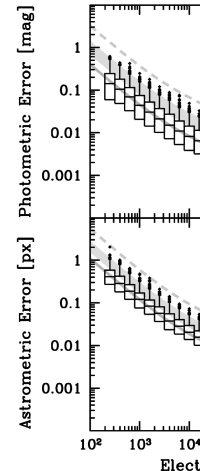
The binned absolute photometric errors are shown as black box-and-whiskers plots (see Appendix A) on the top panel of Fig. 1. The absolute photometric error of an observation is the absolute value of the difference between the measured (estimated) and true (actual) stellar magnitude: $\Delta\mbox{$\mathsf{mag}$}\equiv|\mbox{$\mathsf{mag}$}-\mbox{$\mbox{$\mathsf{mag}$}_{\rm{true}}$}|$. The four grey limits seen on the top panel of Fig. 1 are theoretical predictions (derived from §2.3.4) for the median (50% cumulative fraction: grey solid curve), top hinge (75%: bottom of the grey band), top fence ($\sim$98.35%: top of band), and 5-$\sigma$ outlier ($\sim$99.99997%: grey dashed curve) values. If the rms photometric error is called $\sigma_{\mbox{$\mathsf{mag}$}}$, then the values of these theoretical limits are approximately equal to $0.674\,\sigma_{\mbox{$\mathsf{mag}$}}$, $1.151\,\sigma_{\mbox{$\mathsf{mag}$}}$, $2.398\,\sigma_{\mbox{$\mathsf{mag}$}}$, and $5.423\,\sigma_{\mbox{$\mathsf{mag}$}}$, respectively. If the photometric performance model is correct and mpd has been coded correctly, then (1) the observed median values (central bar in each box) should intersect the theoretical median value, (2) most of the top whiskers should be found inside the band, and (3) most of the outliers should be found above the top of the band and all of the outliers should found below the 5-$\sigma$ outlier limit.

Comparing the absolute photometric errors of the 20,000 simulated CCD observations with the grey theoretical limits, one sees that the photometric performance of the mpd code is very well predicted by the model given in §2.3.4.

The binned total astrometric errors are shown as black box-and-whiskers plots on the bottom panel of Fig. 1. The total astrometric error of an observation is the distance between the measured (estimated) and true (actual) position of a star: $\Delta\mbox{$\mathsf{r}$}\equiv\sqrt{(\mbox{$\mathcal{X}$}\!-\!\mbox{$\mathcal{X}$}_{\rm{true}})^{2}\!+\!(\mbox{$\mathcal{Y}$}-\mbox{$\mathcal{Y}$}_{\rm{true}})^{2}}$. The four grey limits seen on the bottom panel of Fig. 1 are theoretical predictions (derived from §2.4.4) for the median (50% cumulative fraction: grey solid curve), top hinge (75%: bottom of the grey band), top fence ($\sim$98.97%: top of band), and 5-$\sigma$ outlier (99.99997%: grey dashed curve) values. The values of these theoretical limits are approximately equal to $1.178\,\mbox{$\sigma_{\mbox{$\mathcal{X}$}}$}$, $1.666\,\mbox{$\sigma_{\mbox{$\mathcal{X}$}}$}$, $3.027\,\mbox{$\sigma_{\mbox{$\mathcal{X}$}}$}$, and $5.890\,\mbox{$\sigma_{\mbox{$\mathcal{X}$}}$}$, where $\sigma_{\mbox{$\mathcal{X}$}}$ is the rms measurement error for the stellar $\mathcal{X}$ position. If the astrometric performance model is correct and mpd has been coded correctly, then (1) the observed median values should intersect the theoretical median value, (2) most of the top whiskers should be found inside the band, and (3) most of the outliers should be found above the top of the band and all of the outliers should found below the 5-$\sigma$ outlier limit.

Comparing the total astrometric errors of the 20,000 simulated CCD observations with the grey theoretical limits, one sees that the astrometric performance of the mpd code is very well predicted by the model given in §2.4.4.

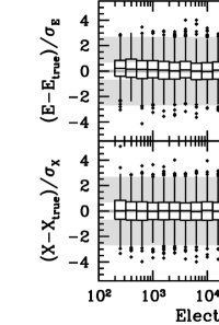
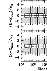
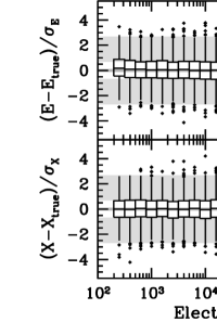
Figure 2 shows the relative stellar intensity errors and the relative $\mathcal{X}$ position errors of the 20,000 stars analyzed in Fig. 1. The relative stellar intensity error is the difference between the measured (estimated) and true (actual) stellar intensity values divided by the estimated stellar intensity error: $\Delta\mbox{$\mathcal{E}$}\equiv(\mbox{$\mathcal{E}$}-\mbox{$\mathcal{E}$}_{\rm{true}})/\mbox{$\sigma_{\mbox{$\mathcal{E}$}}$}$. The relative $\mathcal{X}$ position error is the difference between the measured (estimated) and true (actual) stellar $\mathcal{X}$ position values divided by the estimated $\mathcal{X}$ error: $\Delta\mbox{$\mathcal{X}$}\equiv(\mbox{$\mathcal{X}$}-\mbox{$\mathcal{X}$}_{\rm{true}})/\mbox{$\sigma_{\mbox{$\mathcal{X}$}}$}$. If mpd has been coded correctly, the relative error distributions for the stellar parameters $\mathcal{E}$, $\mathcal{X}$, and $\mathcal{Y}$ should be normally distributed. The five grey limits seen on each panel are theoretical predictions (based on the normal distribution) for, from bottom to top, the bottom fence ($\sim$0.35% cumulative fraction: bottom of the bottom grey band), bottom hinge (25%: top of bottom band), median (50%: grey solid line at zero), top hinge (75%: bottom of top band), top fence ($\sim$99.65%: top of top band) values. If the relative errors for $\mathcal{E}$ and $\mathcal{X}$ are indeed normally distributed, then (1) the observed median values should be near zero, (2) most of the whiskers should be found inside the bands, and (3) most of the outliers should be beyond the fence values.

Comparing the relative errors for $\mathcal{E}$ and $\mathcal{X}$ of the 20,000 simulated CCD observations with the grey theoretical limits, one sees that these errors are, as expected, normally distributed.

• The mpd code works well with oversampled analytical Gaussian PSFs and its performance can be very well predicted with the photometric and astrometric models derived in §2.

5.1.2 Discrete PSFs

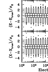
The 20,000 simulated CCD observations analyzed in Figs. 1 and 2 were reanalyzed with mpd using an oversampled discrete Gaussian PSF with a $\mathsf{FWHM}$ of 3.0 px. Figure 3 shows the resultant absolute photometric errors and total astrometric errors. Figure 4 shows the resultant relative errors for $\mathcal{E}$ and $\mathcal{X}$. Notice how similar Figs. 1 and 3 and Figs. 2 and 4 are to each other.

Despite the very different way the shape information of the PSF was encoded (i.e., discrete versus analytical representations), mpd produced nearly identical photometric and astrometric results.

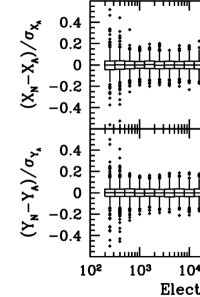
How similar are the measured stellar positions? Figure 5 shows the relative $\mathcal{X}$ and $\mathcal{Y}$ position differences between the previous analytical and numerical analyses with the mpd code. The top panel shows the difference between the numerical $\mathcal{X}$ result and the analytical $\mathcal{X}$ result divided by the estimated error of the analytical result. Similarly, the bottom panel shows the difference between the numerical $\mathcal{Y}$ result and the analytical $\mathcal{Y}$ result divided by the estimated error of the analytical result. The relative differences between the numerical and analytical methods are not normally distributed — observe how much smaller the values on the ordinate of Fig. 5 are compared to those of Figs. 2 and 4. Figs. 2 and 4 are normally distributed and the source of the scatter is photon noise. Figure 5 indicates that the relative differences between the numerical and analytical methods for astrometry are less than one-fifteenth the difference due to photon noise. In other words, the computational noise due to the chosen analysis method (numerical versus analytical) is insignificant when compared to the unavoidable photon noise due to the random arrival of photons in any astronomical CCD observation.

• The mpd code works as well with oversampled discrete Gaussian PSFs as it does with oversampled analytical Gaussian PSFs.

Figure 3: The absolute photometric errors (top) and total astrometric errors (bottom) of $20,000$ simulated CCD stellar observations used in Figs. 1 and 2 were analyzed with mpd using an oversampled discrete Gaussian PSF with a $\mathsf{FWHM}$ of 3.0 px ($\mbox{\boldmath$\beta$}\approx 21.44$ $\mbox{px}^{2};\mbox{V}\equiv 1)$.

Figure 4: Relative stellar intensity errors (top) and relative $\mathcal{X}$ position errors (bottom) of the data set used in Fig. 3.

Figure 5: Relative $\mathcal{X}$ and $\mathcal{Y}$ position differences (top and bottom, respectively) between the numerical (subscript N) and analytical (subscript A) results of the same 20,000 stars used in Figs. 1–4.

Figure 6: The absolute photometric errors (top) and total astrometric errors (bottom) of $20,000$ simulated CCD stellar observations analyzed with mpd using a discrete Gaussian PSF with a $\mathsf{FWHM}$ of 3.0 px with an inefficient detector with $V\!=\!1/9$ $\,(\mbox{\boldmath$\beta$}\approx 1736.79$ $\mbox{px}^{2})$. See the text for more details.

5.1.3 Inefficient Detectors

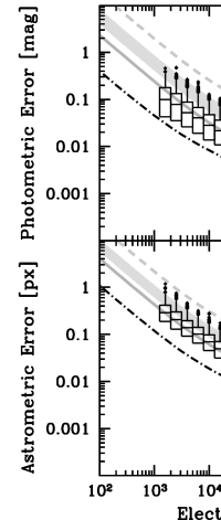
While the volume, V, of the PRF was carefully tracked throughout the derivation of the photometric and astrometric performance models in §2, all previous simulations have assumed a perfect detector $(\mbox{V}\equiv 1)$. Let us now check to see if the effects of a PRF volume integral that is less than one has been correctly accounted for in the performance models of §2 by analyzing simulated observations imaged on a very inefficient detector $(\mbox{V}\ll 1)$.

Twenty thousand oversampled CCD stellar observations were simulated assuming a very inefficient detector with $V=1/9$. Stars were simulated using a discrete Gaussian PSF with a $\mbox{$\mathsf{FWHM}$}\equiv 3$ px located near the center of 60$\times$60 pixels, the input stellar intensities ranged from $-8$ to $-15$ mag ($1585$ to $10^{6}$ $\gamma$); and the observed background sky level was assumed to be a constant value of $\mbox{$\mathcal{B}$}=11.1111$ e^- ($\mbox{$\mathcal{B}$}_{\rm{true}}=100$ $\gamma$, $\langle\mbox{V}\rangle=1/9$) all other simulation parameters were the same as before.

All the simulated observations were analyzed with mpd in the same way as described for the numerical experiment shown in Fig. 3 — except that the volume of the PRF was set to $\mbox{V}=1/9$ in order to simulate the use of an inefficient detector which converts only $\sim$11.1% of photons to electrons.

Figure 6 shows the absolute photometric errors and total astrometric errors of this numerical experiment. The median effective-background area of PRF of these observations was $\mbox{\boldmath$\beta$}\approx 1736.79$ $\mbox{px}^{2}$ which is, as expected, 81 $(=\mbox{V}^{-2})$ times larger than the median value reported in Fig. 3.

Comparing the simulation results with the grey theoretical limits, one sees that the photometric and astrometric performance of the mpd code is very well predicted by the theoretical performance models given in §2.

The black dash-dot curves in each panel of Fig. 6 shows the expected median response with a perfect detector; these curves are the same as the solid grey median curves found in Fig. 3. The observed stellar intensities and observed background sky level are nine times fainter than was seen in the numerical experiment shown in Fig. 3 and the median photometric and astrometric errors in Fig. 6 are, as expected, $\sim$3 $(=V^{-1/2})$ times larger when the inefficient detector is used.

• The mpd code and the theoretical performance models work well with PRFs that have volumes of less than one.

5.2 Undersampled Discrete PSFs

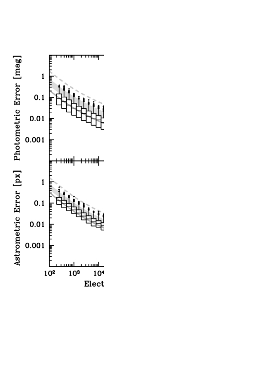
Twenty thousand undersampled CCD stellar observations were simulated using an analytical Gaussian with a $\mbox{$\mathsf{FWHM}$}\equiv 1.5$ px, the other simulation parameters were the same as given in §5.1.1. The median effective-background area of PRF of these observations was $\mbox{\boldmath$\beta$}\approx 6.12$ $\mbox{px}^{2}$ $(\mbox{V}\equiv 1)$. All the simulated observations were analyzed with mpd using a discrete Gaussian PSF with $\mbox{$\mathsf{FWHM}$}\equiv 1.5$ px.

Figure 7 shows the absolute photometric errors and total astrometric errors of this numerical experiment. While the photometric and astrometric results for stars with $\mbox{$\mbox{$\mathcal{E}$}_{\rm{true}}$}\!\la\!30,0000$ e^- are fine, the results for stars brighter than that limit are seen to quickly degrade in accuracy with the brightest stars having median errors that are $\sim$40 times worse than expected.

What starts going wrong at $\mbox{$\mbox{$\mathcal{E}$}_{\rm{true}}$}\approx 30,000$ e^-? Figure 8 shows a one pixel wide slice through a pixel-centered discrete Gaussian PSF with $\mbox{$\mathsf{FWHM}$}=1.5$ px that was shifted half of a pixel in $X$ to the right using damped sinc function given in equation (49). The dashed black curve looks fine, but when expanded by a factor of 100, one sees that negative side lobes have been created due to the fact that the Nyquist-Shannon Sampling Theorem has been violated. Doing a sinc interpolation (damped or otherwise) on undersampled data is never a good idea – the “ringing” seen in Fig. 8 is a classic signature of an edge that is too sharp to be adequately expressed with the limited spatial information contained in an undersampled observation. The biggest negative side lobe of the shifted PSF has a value of about $-$0.0006. Although that may seem to be a small value compared to the total volume integral of one, it is actually quite disastrous because negative PSF values have no physical meaning.

Figure 7: The absolute photometric errors (top) and total astrometric errors (bottom) of $20,000$ simulated CCD stellar observations analyzed with mpd using an undersampled discrete Gaussian PSF with a $\mathsf{FWHM}$ of 1.5 px $(\mbox{\boldmath$\beta$}\approx 6.12$ $\mbox{px}^{2};\mbox{V}\!\equiv\!1)$.

Figure 8: A one pixel wide slice through a pixel-centered discrete Gaussian PSF with $\mbox{$\mathsf{FWHM}$}=1.5$ px that was shifted half of a pixel in $X$ to the right using equation (49). The thick grey curve is the same PSF multiplied by a factor of 100.

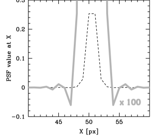
It is now clear what has gone wrong for stars with $\mbox{$\mbox{$\mathcal{E}$}_{\rm{true}}$}\ga 30,000$ e^-. At stellar intensity values greater than 17,000 electrons, the intensity-scaled undersampled PSF models can have negative side lobes that are larger than the rms observed background sky noise level $(\,|$$-$0.0006$|*17,000\,\mbox{e${}^{-}$}=10.2\,\mbox{e${}^{-}$}>10\,\mbox{e${}^{-}$}\approx\sqrt{B})$. At stellar intensity values greater than 167,000 electrons, the observational models have physically nonsensical negative sky values.

• Aliasing (ringing) effects will generally only be seen with bright stars since a large number of photons are required in order to adequately sample the higher spatial frequencies of a PSF.

• Fitting undersampled observations of bright stars with undersampled PSFs results in poor photometry and astrometry.

5.3 Supersampled Discrete PSFs

Figure 9: The absolute photometric errors (top) and total astrometric errors (bottom) of $20,000$ simulated CCD stellar observations analyzed with mpd using a 2$\times$2 supersampled discrete Gaussian PSF with a $\mathsf{FWHM}$ of 1.5 px $(\mbox{\boldmath$\beta$}\approx 6.17$ $\mbox{px}^{2};\mbox{V}\!\equiv\!1)$.

Figure 10: Relative stellar intensity errors (top) and relative $\mathcal{X}$ position errors (bottom) of the data set used in Fig. 9.

A supersampled PSF is a PSF with pixels that have greater spatial resolution (higher spatial frequencies) than the actual pixels in the observational data. For example, a 2$\times$2 supersampled PSF uses 4 pixels to describe every physical pixel of the CCD observation; each supersampled pixel has twice the spatial resolution of the actual pixels in the observation.

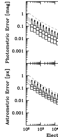
Twenty thousand undersampled CCD stellar observations were simulated using an analytical Gaussian with a $\mbox{$\mathsf{FWHM}$}\equiv 1.5$ px; the other simulation parameters were the same as before. All the simulated observations were analyzed with mpd using a 2$\times$2 supersampled discrete Gaussian PSF with $\mbox{$\mathsf{FWHM}$}\equiv 1.5$ px ($\mbox{\boldmath$\beta$}\approx 6.17$ $\mbox{px}^{2}$; $\mbox{V}\equiv 1$).

Figure 9 shows the absolute photometric errors and total astrometric errors of this numerical experiment. By providing mpd with extra information, in the form of a supersampled PSF, the Nyquist-Shannon Sampling Theorem was no longer violated and excellent photometry and astrometry was done with this undersampled data set.

Figure 10 shows the relative errors for $\mathcal{E}$ and $\mathcal{X}$. The relative stellar intensity errors are normally distributed. However, the relative $\mathcal{X}$ position errors are almost, but not quite, normally distributed. The mpd code is accurately measuring the stellar positions (i.e., the median difference, $\mbox{$\mathcal{X}$}-\mbox{$\mathcal{X}$}_{\rm{true}}$, values are zero) but the rms position error estimates ($\sigma_{\mbox{$\mathcal{X}$}}$) are slightly underestimated (the top and bottom whiskers for $\mbox{$\mbox{$\mathcal{E}$}_{\rm{true}}$}\ga 10,000$ e^- are seen to extend beyond the grey bands). The same effect is seen with $\mathcal{Y}$. Using a higher-resolution supersampled PSF (3$\times$3, 4$\times$4, $\ldots$) does not eliminate the small underestimation by mpd of position errors. The position errors estimated by mpd are close to the photonic limit, but the actual errors — for undersampled observations — are close to the astrometric CRLB with square CCD pixels (Winick, 1986).

• Accurate and precise CCD stellar photometry and astrometry may be obtained with undersampled CCD observations if supersampled PSFs are used during the PSF-fitting process.

5.4 Critically-Sampled Discrete PSFs

Let us now investigate what happens when critically-sampled data is fit with a critically-sampled PSF.

Twenty thousand critically-sampled CCD stellar observations were simulated using an analytical Gaussian with a $\mbox{$\mathsf{FWHM}$}\equiv 2.35482$ px; the other simulation parameters were the same as before. All the simulated observations were analyzed with mpd using a critically-sampled discrete Gaussian PSF with $\mbox{$\mathsf{FWHM}$}\equiv 2.35482$ px ($\mbox{\boldmath$\beta$}\approx 13.62$ $\mbox{px}^{2}$; $\mbox{V}\equiv 1$).

Figure 11 shows the absolute photometric errors and total astrometric errors of this numerical experiment. Figure 12 shows the relative errors for $\mathcal{E}$ and $\mathcal{X}$. Looking carefully at Figs. 11 and 12, one sees that the photometric and astrometric performance is well matched to the theoretical expectations except for the brightest three bins ($\mbox{$\mbox{$\mathcal{E}$}_{\rm{true}}$}\ga 316,000$ e^-).

Figure 11: The absolute photometric errors (top) and total astrometric errors (bottom) of $20,000$ simulated CCD stellar observations analyzed with mpd using critically-sampled discrete Gaussian PSF with a $\mathsf{FWHM}$ of 2.35482 px $(\mbox{\boldmath$\beta$}\approx 13.62$ $\mbox{px}^{2};\mbox{V}\!\equiv\!1)$.

Figure 12: Relative stellar intensity errors (top) and relative $\mathcal{X}$ position errors (bottom) of the data set used in Fig. 11.

Twenty thousand critically-sampled CCD stellar observations were simulated using an analytical Gaussian with a $\mbox{$\mathsf{FWHM}$}\equiv 2.35482$ px; the other simulation parameters were the same as before. All the simulated observations were analyzed with mpd using a 2$\times$2 supersampled discrete Gaussian PSF with $\mbox{$\mathsf{FWHM}$}\equiv 2.35482$ px ($\mbox{\boldmath$\beta$}\approx 13.62$ $\mbox{px}^{2}$; $\mbox{V}\equiv 1$).

Figure 13 shows the absolute photometric errors and total astrometric errors of this numerical experiment. Figure 14 shows the relative errors for $\mathcal{E}$ and $\mathcal{X}$. The photometric and astrometric performance is well matched to the theoretical expectations for all stellar intensities.

Figure 13: The absolute photometric errors (top) and total astrometric errors (bottom) of $20,000$ simulated CCD stellar observations analyzed with mpd using a 2$\times$2 supersampled discrete Gaussian PSF with a $\mathsf{FWHM}$ of 2.35482 px $(\mbox{\boldmath$\beta$}\approx 13.62$ $\mbox{px}^{2};\mbox{V}\!\equiv\!1)$.

Figure 14: Relative stellar intensity errors (top) and relative $\mathcal{X}$ position errors (bottom) of the data set used in Fig. 13.

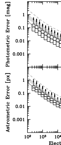
Comparing Fig. 7 with Fig. 9 and Fig. 11 with Fig. 13, one sees that one can obtain excellent stellar photometry and astrometry with the MATPHOT algorithm for all stellar intensities – even if the observational data is undersampled – as long as the discrete PSFs used to do the model fitting are sampled finely enough to have sufficient spatial frequency coverage such that the Nyquist-Shannon Sampling Theorem is not violated.

Comparing Fig. 3 with Fig. 11, one sees that the breakpoint for the MATPHOT algorithm between undersampled and oversampled data is $13.62<\mbox{\boldmath$\beta$}\leq 21.44$ $\mbox{px}^{2}$ or, in terms of a Gaussian Full-Width-at Half Maximum, $2.35482\la\mbox{$\mathsf{FWHM}$}\leq 3$ px.

• If a discrete PSF is close to being critically sampled, then one should use a supersampled discrete PSF which is oversampled in terms of supersampled pixels $(\mbox{spx})$. In other words, if the equivalent-background area is less than 21 square pixels ($\mbox{\boldmath$\beta$}<21$ $\mbox{px}^{2}$; Gaussians: $\mbox{$\mathsf{FWHM}$}<3.0$ px), then one should use a supersampled discrete PSF which has an equivalent-background area of at least 21 square supersampled pixels ($\mbox{\boldmath$\beta$}\geq 21$ $\mbox{spx}^{2}$; Gaussians: $\mbox{$\mathsf{FWHM}$}\geq 3.0$ spx).

5.5 Ugly Discrete PSFs

Let us now investigate the photometric and astrometric performance of the MATPHOT algorithm with an ugly (realistic) space-based PSF.

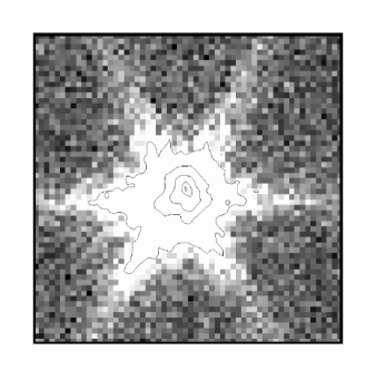
Figure 15 shows a simulated Next Generation Space Telescope (NGST) $V$-band CCD stellar observation. This simulated observation used a 2$\times$2 supersampled PSF which was based on a 8-meter TRW-concept $1.5\,\mu$ diffraction-limited primary mirror with 1/13 wave rms errors at $1.5\,\mu$; the original version of the PSF was kindly provided by John Krist (STScI). The six-sided “snowflake” pattern seen in Fig. 15 is mainly due to fact that the primary mirror is composed of segmented hexagonal-shaped mirrors. Observers will note that this PSF is very similar to optical PSFs seen with the 10-m telescopes at the W. M. Keck Observatory. The 6.5-m James Webb Space Telescope (JWST) is likely to have similar looking near-infrared PSFs once it achieves first light in $\sim$2011.

The NGST PSF is so complicated that it is unlikely that it could be represented adequately with a continuous analytical mathematical function. Space-based observations frequently have high spatial frequencies which make them ideal candidates for photometric and astrometric analysis using discrete PSFs.

Figure 15: A simulated $V$-band Next Generation Space Telescope image based on a 2$\times$2 supersampled PSF model for a 8-meter TRW-concept 1.5-micron diffraction-limited primary mirror with 1/13 rms wave errors. Contour levels of 90%, 50%, 10%, 1%, and 0.1% of the peak intensity are shown with black curves. The pixel scale is 0.0128 arcsec $\mbox{px}^{\,-1}$. This image uses a linear stretch with a pixel intensity mapping of black for $\la\,70$ e^- and white for $\ga\,150$ e^-.

Twenty thousand CCD stellar observations were simulated using the simulated $V$-band NGST 2$\times$2 supersampled PSF described above; the other simulation parameters were the same as before. All the simulated observations were analyzed with mpd with the PSF used to create the simulated observations.

Figure 16: The absolute photometric errors (top) and total astrometric errors (bottom) of $20,000$ simulated CCD stellar observations analyzed with mpd using the 2$\times$2 supersampled NGST PSF described in Fig. 15 $(\mbox{\boldmath$\beta$}\approx 31.25$ $\mbox{px}^{2};\mbox{V}\!\equiv\!1)$.

Figure 17: Relative stellar intensity errors (top) and relative $\mathcal{X}$ position errors (bottom) of the data set used in Fig. 16.

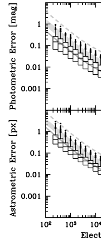
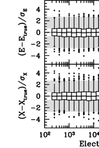
Figure 16 shows the absolute photometric errors and total astrometric errors of this numerical experiment. Figure 17 shows the relative errors for $\mathcal{E}$ and $\mathcal{X}$. The photometric and astrometric performance is well matched to the theoretical expectations for all stellar intensities.

Although only Gaussian PSFs were used in previous numerical experiments, the excellent fit seen in the top panel of Fig. 16 between the theoretical photometric performance model (§2.3.4) and actual mpd measurements using such an ugly discrete PSF is not surprising once one remembers that the theoretical photometric performance model was derived from an abstract Point Response Function.

The development of the theoretical astrometric performance model, however, required differentiation of the Point Response Function which I assumed to be an oversampled analytical Gaussian function. The analytical Gaussian bright star astrometric limit was transformed to the general form by assuming that the Gaussian-specific $\mbox{$\mathcal{S}$}^{2}$ term could be replaced with the more general $\mbox{$\mathcal{L}$}^{2}$ term, which, by definition, can be computed for any PRF. The same assumption was then used to derive the general faint star astrometric limit. The excellent fit seen in the bottom panel of Fig. 16 indicates that this bold assumption is not only useful but practical. Many numerical experiments with very ugly discrete PSFs have shown that the theoretical astrometric performance model of §2.4.4 works well with ugly discrete Point Response Functions.

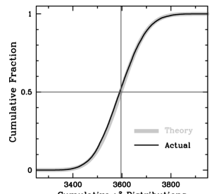
If the MATPHOT algorithm is optimally extracting photometric and astrometric information from a stellar observation, and mpd has been correctly coded, and the CCD observation has been properly calibrated, and the PRF used in the observational model is correct, and accurate estimates of the measurements errors for each pixel have been made, then one expects that the $\chi^{2}$ goodness-of-fit value reported by mpd to be distributed as a $\chi^{2}$ distribution with the number of degrees of freedom equal to the difference between the number of pixels in the observation and the number of free parameters. Figure 18 shows that this prediction about the precision and accuracy of the MATPHOT algorithm has been verified: the cumulative distribution of the $\chi^{2}$ reported by mpd (thin black curve) is seen to lie on top of the cumulative $\chi^{2}$ distribution of for 3596 [$=$ $60^{2}$ pixels $-$ 4 free parameters $(\mbox{$\mathcal{E}$}$, $\mathcal{X}$, $\mathcal{Y}$, and $\mbox{$\mathcal{B}$})$ ] degrees of freedom (thick grey curve).

Figure 18: A comparison between the cumulative $\chi^{2}$ distribution for 3596 degrees of freedom (thick curve) and the measured $\chi^{2}$ value (thin curve), of the data set used in Fig. 16, reported by the mpd implementation of the MATPHOT algorithm.

• The mpd code works well with ugly discrete PSFs and its performance can be well predicted using the general theoretical photometric and astrometric performance models given in §2.

• The $\chi^{2}$ goodness-of-fit value reported by mpd is a statistically reliable measure of the quality of a photometric and astrometric reduction of a stellar observation obtained with the MATPHOT algorithm using ugly discrete PSFs.

5.6 Ugly Detectors

Let us now investigate the photometric and astrometric performance of the MATPHOT algorithm with an ugly PSF and an ugly detector.

Suppose one has a detector where every pixel has been divided up into 16 square regions called “subpixels”. Let us call the first row and first column of subpixels “gate structures” which are optically inactive with 0% QE. The remaining 9 subpixels are the optically active part of the pixel with a 100% QE. By definition, such a pixel would have a very large intrapixel QE variation with only 56.25% of the total pixel area being capable of converting photons to electrons.

A few extra lines of code were added to the mpd program to simulate the image formation process with such an ugly detector. The new version of mpd is called mpdx and was designed specifically for use with 4$\times$4 supersampled PSFs.

Ten thousand CCD stellar observations of $-13$ mag stars ($\sim$$2.512^{13}$ $\gamma$) were simulated and analyzed with mpdx using a 4$\times$4 supersampled version of the simulated $V$-band NGST PSF described above. The observed background level was assumed to be a constant value of $\mbox{$\mathcal{B}$}=56.25$ e^- ($\mbox{$\mathcal{B}$}_{\rm{true}}=100$ $\gamma$, $\langle\mbox{V}\rangle=0.5625$) and all other simulation parameters were the same as before. The measured PRF volume of these simulated observations was $\mbox{V}=0.5616\pm 0.0185$ which is consistent with the expected value of 0.5625 from the physical structure of a single pixel. The median and semiquartile range of the effective-background area $(\mbox{\boldmath$\beta$})$ of these observations was, respectively, 28.10 and 4.82 $\mbox{px}^{2}\,$. The median critical-sampling scale length of these observations was $\mbox{$\mathcal{L}$}\approx 0.8398$ px — indicating that these observations were undersampled, as expected.

The optically inactive gate structures of the pixel cause the observed number of electrons in each stellar image to be significantly less than the number of photons which fell on the detector. The total amount of loss was dependent on where the center of the star fell within the central pixel of the stellar image. Figure 19 shows that stars centered in the middle of the active area of a pixel suffered a $\sim$40% loss ($\Delta m\approx 0.56$ mag) while those centered on gate structures (grey points) lost up to 47% ($\Delta m\approx 0.69$ mag).

Although this numerical experiment may seem to be very artificial, large intrapixel sensitivity variations can be found in cameras currently installed on the Hubble Space Telescope. Lauer (1999) reported peak-to-peak variations of 0.39 mag at the $J$ band (F110W) and 0.22 mag at the $H$ band (F160W) of the NIC3 camera of the HST NICMOS instrument. The peak-to-peak variation of $\sim$0.2 mag at F160W with NIC 3 was independently confirmed by Hook & Fruchter (2000).

Figure 19: The measured electron loss of the 10,000 simulated CCD observations of $-13$ mag stars analyzed with mpdx using a 4$\times$4 supersampled version of the NGST PSF. The electron loss is plotted as a function of the absolute value of the distance from the center of a star and the center of the active region of the central pixel of the stellar image.

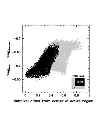
The mean observed stellar magnitude for these $-13$ mag stars was $-12.3728\pm 0.0359$ mag. The photometric performance model predicts an rms measurement error of $0.0036$ mag for these bright stars. With an average loss of 44% and an rms measurement error that is ten times larger than expected from photon statistics, the observed stellar magnitudes were neither precise or accurate.

Figure 20 shows that mpdx was able to do an excellent job in recovering the true stellar magnitude of the 10,000 $-13$ mag stars — despite being presented with a worst-case scenario of undersampled observations with an ugly PSF imaged on an ugly detector with a very large intrapixel QE variation.

Figure 20: The observed (left) and the measured (right) stellar magnitude distributions of the 10,000 $-13$ mag stars described in Fig. 19.

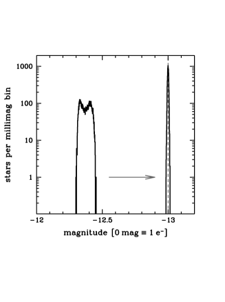
The mean measured stellar magnitude reported by mpdx was $-12.9998\pm 0.0039$ mag and the mean rms error estimated by mpdx was $0.00384\pm 0.00006$ mag. The photometric performance of mpdx is fully consistent with theoretical expectations — which were derived for an ideal detector with no intrapixel QE variation.

Twenty thousand CCD stellar observations were simulated and analyzed with mpdx using the same 4$\times$4 supersampled version of the simulated $V$-band NGST PSF. The input stellar intensities ranged from $-6$ to $-15$ mag ($251$ to $10^{6}$ $\gamma$). The observed background level was assumed to be a constant value of $\mbox{$\mathcal{B}$}=56.25$ e^- ($\mbox{$\mathcal{B}$}_{\rm{true}}=100$ $\gamma$, $\langle\mbox{V}\rangle=0.5625$) and all other simulation parameters were the same as before. The median and semiquartile range of the effective-background area $(\mbox{\boldmath$\beta$})$ of these observations was, respectively, 28.04 and 4.77 $\mbox{px}^{2}\,$.

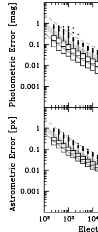
Figure 21 shows the absolute photometric errors and total astrometric errors of this numerical experiment. Comparing the simulation results with the grey theoretical limits, one sees that the photometric and astrometric performance of the mpdx code is well predicted by the theoretical performance models given in §2.

Figure 21: The absolute photometric errors (top) and total astrometric errors (bottom) of $20,000$ simulated CCD stellar observations analyzed with mpdx using a 4$\times$4 supersampled version of the NGST PSF $(\mbox{\boldmath$\beta$}\approx 28.04$ $\mbox{px}^{2};\mbox{V}\!=\!0.5625)$.

• Excellent stellar photometry and astrometry is possible with ugly PSFs imaged onto ugly detectors as long as the image formation process within the detector is accurately modeled by the photometric reduction code.

6 Discussion

After developing theoretical photometric and astrometric performance model for Point Spread Function (PSF)-fitting stellar photometry, I described the unique features of the MATPHOT algorithm for accurate and precise stellar photometry and astrometry using discrete Point Spread Functions. I conducted numerical experiments with the mpd implementation of the MATPHOT algorithm and demonstrated that the computational noise due to the chosen analysis method (numerical versus analytical) is insignificant when compared to the unavoidable photon noise due to the random arrival photons in any astronomical CCD observation. The MATPHOT algorithm was specifically designed for use with space-based stellar observations where PSFs of space-based cameras frequently have significant amounts of power at higher spatial frequencies. Using simulated NGST CCD observations, I demonstrated millipixel relative astrometry and millimag photometry is possible with very complicated space-based discrete PSFs.

The careful reader will observe that I have not discussed how a discrete PSF is derived. The MATPHOT algorithm will optimally determine the brightness and position of a star in a CCD observation when provided with the correct PSF and DRF — functions which need to be determined beforehand through calibration procedures. Photometric and astrometric accuracy and precision degrades if either the PSF or DRF is poorly known. PSF reconstruction (calibration) is a complicated topic in its own right and has been the subject of many articles, instrumentation reports, and entire workshops. The challenges of PSF reconstruction are many. An astronomer may be faced with trying to derive a PSF from an observation

• with a variable PSF within the field of view,

• that has too few bright stars,

• that might be undersampled,

• that might be poorly dithered,

• that might be poorly flat-fielded,

• that exhibits significant charge transfer efficiency variations,

• that has variable charge diffusion within the CCD substrate,

• with significant photon loss due to charge leakage,

• that might not actually be linear below the 1% level.

While many of these problems can be overcome by the proper design of instruments or experiments, their solution is beyond the scope of this article which has sought to determine the practical limits of PSF-fitting stellar photometry.

The analysis presented in this article has assumed that PSFs are perfectly known – a situation that is rarely, if ever, physically possible. The cores of observationally based PSFs are generally much better determined than the broad wings due to simple photon statistics. The effect of large instrumental calibration errors can also be significant. For example, flat-field limitations can dramatically impact the achievable levels of photometric and astrometric precision. An investigation based on theory of the effect of PSF errors and flat-field calibration error on the limits of PSF-fitting stellar photometry would be very difficult. An investigation based on numerical experiments, however, might be a much more tractable proposition. In any case, a through investigation of the effects of calibration errors on the limits of PSF-fitting stellar photometry is best left to another article.

I would like to thank the anonymous referee whose careful reading and insightful comments have improved this article. Special thanks are due to Ian Roederer who checked all of the mathematical proofs in an early draft of the manuscript. Jessica Moy has my heartfelt thanks for cheerfully helping me acquire copies of many articles in technical journals that are not available in the NOAO library collection. I would also like to thank the following people for providing stimulating conversations, encouragement, and support during the extensive research and development effort behind the creation of the MATPHOT algorithm and and its various software implementations: Joseph Bredekamp, Susan Hoban, Dot Appleman, Taft Armandroff, Nick Buchholz, Marc Buie, Harvey Butcher, Julian Christou, Chuck Claver, Lindsey Davis, Michele De Le Peña, Mike Fitzpatrick, Ken Freeman, Dan Golombek, Richard Green, Steve Howell, George Jacoby, Buell Jannuzi, Stuart Jefferies, Ivan King, John Krist, Todd Lauer, John MacKenty, John Mather, Mike Merrill, Dave Monet, Mark Morris, Jeremy Mould, Jan Noordam, John Norris, Sudhakar Prasad, the late Alex Rogers, Steve Ridgway, Pat Seitzer, James Schombert, Donald West, and Sidney Wolff. This research has been supported in part by the following organizations, institutions, and research grants (in reverse chronological order): National Aeronautics and Space Administration (NASA), Interagency Order No. S-13811-G, which was awarded by the Applied Information Systems Research Program (NRA 01-OSS-01) of NASA’s Science Mission Directorate, Interagency Order No. S-67046-F which was awarded the Long-Term Space Astrophysics Program (NRA 95-OSS-16) of NASA’s Office of Space Science, Center for Adaptive Optics (CfAO), Institute for Pure and Applied Mathematics (IPAM), Kitt Peak National Observatory, National Optical Astronomy Observatory, Association of Universities for Research in Astronomy Inc. (AURA), National Science Foundation, Mount Stromlo and Siding Spring Observatories, Australian National University, the Netherlands Foundation for Astronomical Research (ASTRON), and the Netherlands Organization for the Advancement of Pure Research (ZWO), and the Kapteyn Astronomical Institute of Groningen.

Appendix A Box-and-Whisker Plots

A box-and-whisker plot (a.k.a. box plot) is a graphical method of showing a data distribution. A box is drawn showing the inner quartile range of the data which, by definition, includes half of all the data values (see Fig. 22). The median of the data is shown with a bar inside the box. The bottom end of the box is the lower quartile (25%) of the data; Tukey (1977), the creator of the box-and-whiskers plot, calls this value the lower hinge, $\mathsf{LH}$, value. The top end of the box is the upper quartile (75%) of the data which is called the upper hinge, $\mathsf{UH}$, value. The step value is 1.5 times the inner quartile range: $\mbox{$\Delta$}\equiv 1.5*(\mbox{$\mathsf{UH}$}-\mbox{$\mathsf{LH}$})$. The top fence value is the sum of the upper hinge and step values: $\mbox{$\mathsf{TF}$}\equiv\mbox{$\mathsf{UH}$}+\mbox{$\Delta$}$. The bottom fence value is the difference between the lower hinge and step values: $\mbox{$\mathsf{BF}$}\equiv\mbox{$\mathsf{LH}$}-\mbox{$\Delta$}$. The top whisker is drawn from the upper hinge value to the largest data value that is less than or equal to the top fence value: $\mbox{$\mathsf{TW}$}\leq\mbox{$\mathsf{TF}$}$. Similarly, the bottom whisker is drawn from the lower hinge value to the smallest data value that is greater than or equal to the bottom fence value: $\mbox{$\mathsf{BW}$}\geq\mbox{$\mathsf{BF}$}$. Data values that are greater than the top fence value or less than the bottom fence value are called outliers and are plotted at their appropriate value beyond the whiskers. For a normal distribution, which is a Gaussian distribution with a mean of zero and a standard deviation of one, the bottom fence, bottom hinge, median, top hinge and top fence values are, respectively, $-$2.6980 (0.35% cumulative fraction), $-$0.6745 (25%), zero (50%), 0.6745 (75%), 2.6980 (99.65%).

Figure 22: A box-and-whiskers plot of a data set of 1000 normal deviates. See the text for details.

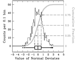
Figure 22 shows a data set of 1000 normal deviates. The histogram of the data with 0.1-wide bins is shown with thin black lines. The cumulative fraction distribution of the data is shown as a thick gray curve. The box-and-whisker plot of the data is shown with thick black lines below the histogram; arrows show the relationship between various box values and the cumulative fraction distribution. The mean and standard deviation of this data set are, $-$0.0341 and 0.9739, respectively. The bottom fence, bottom whisker, bottom hinge, median, top hinge, top whisker, and top fence values of this data set are, respectively, $-$2.5511 (0.25% cumulative fraction), $-$2.4940 (0.30%), $-$0.6522 (25.10%), $-$0.0231 (50.00%), 0.6137 (75.10%), 2.4580 (99.50%), 2.5126 (99.57%). The seven outlier values of this data set, $-$2.9500, $-$2.6320, 2.5390, 2.7150, 2.7430, 2.8270, 2.8530, are plotted in Fig. 22 as diamonds beyond the whiskers.

References

- Abramowitz & Stegun (1964) Abramowitz, M., & Stegun, I. 1964, Handbook of Mathematical Functions with Formulas, Graphs, and Mathematical Tables, Applied Mathematics Series, 55, eds. M. Abromowitz and I. Stegun (Washington, D.C.: NBS)
- Arfken (1970) Arfken, G. B. 1970, Mathematical Methods for Physicists, 2nd ed., (New York: Academic Press)
- Biretta et al. (2001) Biretta, J., et al. 2001, WFPC2 Instrument Handbook, Version 6.0 (Baltimore: STScI)
- Hook & Fruchter (2000) Hook, R. N., & Fruchter, A. S. 2000, in ASP Conf. Ser., Vol. 216, Astronomical Data Analysis Software and Systems IX, eds. N. Manset, C. Veillet, and D. Crabtree (San Francisco: ASP), 521
- Irwin (1985) Irwin, M. J. 1985, MNRAS, 214, 575
- Jakobsen, Greenfield, & Jedrzejewski (1992) Jakobsen, P., Greenfield, P., & Jedrzejewski, R. 1992, A&A, 253, 329
- King (1971) King, I. R. 1971, PASP, 83, 199
- King (1983) King, I. R. 1983, PASP, 95, 163
- Lauer (1999) Lauer, T. R. 1999, PASP, 111, 1434
- Levenberg (1944) Levenberg, K. 1944, Q. App. Math., 2, 164
- Marquardt (1963) Marquardt, D. 1963, J. SIAM, 11, 431
- Mighell (1989) Mighell, K. J. 1989, MNRAS, 238, 807
- Mighell (1999) Mighell, K. J. 1999, in ASP Conf. Ser., Vol. 172, Astronomical Data Analysis Software and Systems VIII, eds.D. M. Mehringer, R. L. Plante, and D. A. Roberts (San Francisco: ASP), 317
- Mighell (2002) Mighell, K. J. 2002, in Proceedings of SPIE, Vol. 4847, Astronomical Data Analysis II, eds. J.-L. Starck and F. D. Murtagh (Bellingham, WA: SPIE), 207
- Pogson (1856) Pogson, N. 1856, MNRAS, 17, 12
- Perryman et al. (1989) Perryman, M. A. C, Jakobsen, P., Colina, L., Lelievre, G., Macchetto, F., Nieto, J. L., & di Serego Alighieri, S. 1989, A&A, 215, 195
- Press et al. (1986) Press, W. H., Flannery, B. P., Teukolsky, S. A., & Vetterrling W. T. 1986, Numerical Recipes. The Art of Scientific Computing (Cambridge: Cambridge University Press)
- Tukey (1977) Tukey, J. W. 1977, Exploratory Data Analysis, (Reading, MA: Addison-Wesley)
- Wells, Greisen, & Harten (1981) Wells, D. C., Greisen, E. W., & Harten, R. H. 1981, A&AS, 44, 363
- Winick (1986) Winick, K. A. 1986, JOSA A, 3, 1809