KASCADE measurements of energy spectra for elemental groups of cosmic rays: Results and open problems

Abstract

A composition analysis of KASCADE air shower data is performed by means of unfolding the two-dimensional frequency spectrum of electron and muon numbers. Aim of the analysis is the determination of energy spectra for elemental groups representing the chemical composition of primary cosmic rays. Since such an analysis depends crucially on simulations of air showers the two different hadronic interaction models QGSJet and SIBYLL are used for their generation. The resulting primary energy spectra show that the knee in the all particle spectrum is due to a steepening of the spectra of light elements but, also, that neither of the two simulation sets is able to describe the measured data consistently over the whole energy range with discrepancies appearing in different energy regions.

, , , , , , , , , , , , , , , , , , , , , , , , , , , , , , , , , , , , , , , , , , ,

=

1 Introduction

The energy spectrum of primary cosmic rays, extending over more than 12 decades in energy, follows, over a large range, a simple power law $dJ/dE$ $\propto E^{\gamma}$ indicating its non-thermal character. However, in the region between 1 PeV and 10 PeV a change of the spectral index from $\gamma\approx-2.65$ to $\gamma\approx-3.1$ occurs, the so-called knee in the spectrum of cosmic rays. Since its discovery [1] nearly 50 years ago many measurements have been performed in this energy range (see e.g. [2] for recent measurement results), but the origin of the knee feature is still not convincingly explained.

Proposals for its origin range from astrophysical scenarios like the change of acceleration mechanisms [3, 4, 5] at the sources of cosmic rays (supernova remnants, pulsars, etc.) or effects due to the propagation [6, 7] inside the Galaxy (diffusion, drift, escape from the Galaxy) to particle physics models like the interaction with relic neutrinos [8] during transport or new processes in the atmosphere [9, 10] during air shower development. Common to all models is the prediction of a change of composition over the knee region. Moreover, in order to distinguish between individual models, knowledge of the energy spectra of individual elements or at least mass groups of primary cosmic rays is desired since the different models predict different spectral shapes.

Because of the low fluxes of cosmic rays only indirect measurements via the detection of extensive air showers (EAS) induced by primary cosmic ray particles in the atmosphere are feasible at present in the energy range close to and above 1 PeV. Determination of spectra for individual elements or mass groups is limited by the large intrinsic fluctuations of EAS observables. Furthermore, any analysis of air shower data has to rely on EAS simulations and our limited knowledge of particle physics in the energy range of relevance. Since the primary energies of the showers are beyond the energy range of man-made accelerators and reactions relevant to shower development occur in the very forward direction not accessible in collider experiments, uncertainties in the description of hadronic interactions in shower development are unavoidable. One has, therefore, to rely on the use of phenomenological interaction models which differ in their predictions in some respect strongly, making the task of retrieving information about individual energy spectra from air shower data even more difficult. Approaches facing these difficulties by using statistical methods and extensive comparisons with simulations can be found e.g. in [11, 12].

In this paper we present an analysis of the classical EAS observables, electron and muon numbers, which deals with these problems. Because of the high accuracy of the KASCADE experiment the presented method, based on unfolding procedures, is capable of reconstructing energy spectra for five elements representing different mass groups of primary cosmic ray particles. The analysis is performed twice using simulations with two different high energy hadronic interaction models, QGSJet [13] and SIBYLL [14]. This approach gives also a lower limit of the uncertainties due to the modelling of hadronic interactions. It turns out that the analysis is sensitive to the different models allowing to identify inconsistencies between simulations and data and to give hints to improve the models.

After a brief description of the experimental setup and the data used in Section 2 the idea and the approach of the analysis are outlined in Section 3. Here the main objective is the formulation of the relation between the measured two-dimensional shower size spectrum and the primary energy spectra as matrix equation. Mathematical details of this procedure are given in Appendix A.1. In this equation all relevant EAS and reconstruction properties are contained in the so-called response matrix. Section 4 deals with the description of the distributions necessary for the calculation of the matrix elements. In Section 5 unfolding as a method for solving the matrix equation is introduced whereas in Section 6 its application to Monte Carlo data is discussed. The results of the unfolding analysis applied to measured data are presented in Section 7 and discussed in Section 8, followed by the conclusions.

2 The KASCADE experiment and data selection

The KASCADE (Karlsruhe Shower Core and Array Detector) experiment [15] investigates air showers in a primary energy range from 100 TeV to 100 PeV and measures a large number of observables for each event: electrons, muons at four energy thresholds, and energy and number of hadrons. The main detector components of KASCADE are the field array [15], the central detector [16, 17], and the muon tracking detector [18]. In the present analysis only data from the field array is used. Detailed descriptions of the experimental setup and reconstruction procedures of the main shower observables can be found in [15, 19].

The field array measures electrons and muons ($E_{\mu}>230$ MeV) in the shower separately using an array of 252 detector stations containing shielded and unshielded detectors, arranged on a square grid of $200\times 200$ m² with a spacing of 13 m. These stations are organized in 16 so-called clusters, each consisting of 16 stations in the outer part and 15 stations in the inner part of the array, respectively. Fig. 1 displays a sketch of the installation and of a detector station.

Figure 1: Left: layout of the KASCADE air shower experiment. Right: sketch of a detector station with shielded and unshielded scintillation detectors.

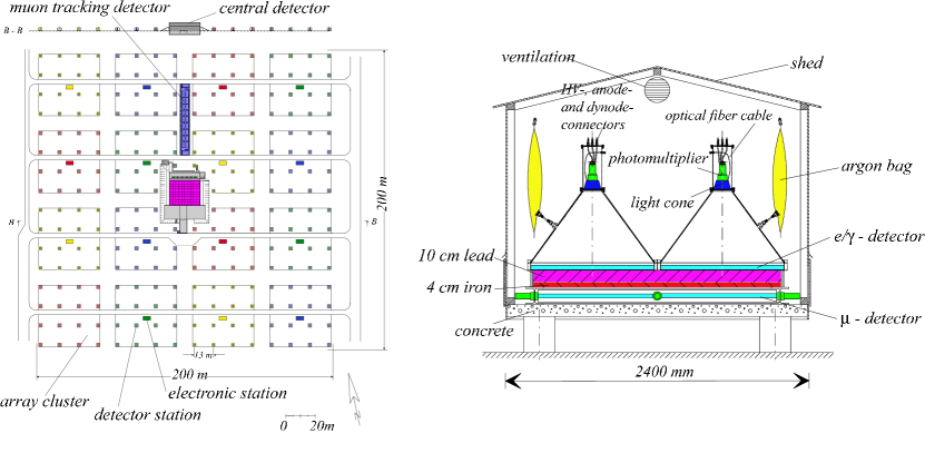
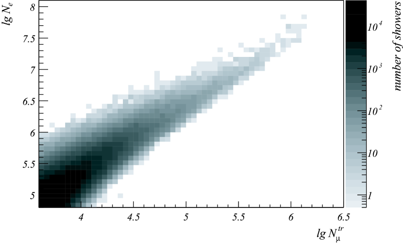
The array observables used in the following are the total electron number $N_{e}$ and the truncated muon number $N_{\mu}^{tr}$. The latter is the number of muons with distances to the shower core between 40 m and 200 m. Input of the analysis is the two-dimensional shower size distribution with respect to these two observables. It is displayed in Fig. 2. The zenith angle of the showers in the analysis is restricted to values between $0^{\circ}$ and $18^{\circ}$. In order to ensure a high quality of the reconstructed shower observables the following cuts are applied:

• The location of the reconstructed shower core has to lie inside a circle of 91 m radius around the center of the array. In this way an erroneous reconstruction of showers with cores outside the array can be mostly avoided.

• The reconstructed age-parameter $s$ of the fit with the NKG-function to the lateral distribution of electrons has to be inside the interval $0.2<s<2.1$. Values larger or smaller correspond to poorly reconstructed showers which are mostly small but may be reconstructed with large shower sizes [19].

• Only measurement runs with all clusters active are considered. Missing clusters during measurement strongly influence the measurement and reconstruction thresholds.

• To avoid threshold effects only showers with showers sizes $\lg N_{e}\geq 4.8$ and $\lg N_{\mu}^{tr}\geq 3.6$ are included.

The total number of events remaining after these cuts amounts to $6.9\cdot 10^{5}$ and the effective measurement time adds up to 900 days. This rather small number of remaining showers is due to the severe cuts applied in order to guarantee a high data quality. As will be seen in the following, the remaining statistical base is sufficient and not the limiting factor for the reliability of the results.

Figure 2: Two-dimensional shower size spectrum used in the analysis. The range in $\lg N_{e}$ and $\lg N_{\mu}^{tr}$ is chosen to avoid influences of inefficiencies.

3 Outline of the analysis

Starting point of the analysis is the two-dimensional shower size spectrum and the contents (number of events) of the histogram cells displayed in Fig. 2. In the following each cell of the shower size spectrum is labeled by a single index $i$ for identification. The number of events in each cell $i$ results from the superposition of contributions induced by different primary particles with various energies. In this sense information about the primary energy spectra of all particle types is present in each cell and the analyzing task is to disentangle this information.

Mathematically the content of a specific cell $i$ of the two-dimensional spectrum, i.e. the number of showers $N_{i}$ with shower sizes $(\lg N_{e},\lg N_{\mu}^{tr})_{i}$ of cell $i$, is related to the flux of primary cosmic ray elements via the integral equation:

$$N_{i}=2\pi A_{s}T_{m}\sum_{A=1}^{N_{A}}\int_{0^{\circ}}^{18^{\circ}}\int_{-\infty}^{+\infty}\frac{{\mathrm{d}}J_{A}}{{\mathrm{d}}\lg E}\/p_{A}((\lg N_{e},\lg N_{\mu}^{tr})_{i}|\lg E)\sin\theta\cos\theta\,{\mathrm{d}}\lg E\,{\mathrm{d}}\theta$$ (1)

where ${\mathrm{d}}J_{A}/{\mathrm{d}}\lg E$ denotes the differential flux of an element with mass number $A$ and the summation is carried out for all elements present in the primary cosmic radiation. The conditional probability $p_{A}$ describes the probability to measure a shower of primary energy $\lg E$ and primary mass $A$ with shower sizes $(\lg N_{e},\lg N_{\mu}^{tr})_{i}$. Measurement time $T_{m}$ and sampling area $A_{s}$ can be treated as constants. For the data range considered no dependence on azimuth angle is found which results in the factor of $2\pi$. Any dependence on solid angle is therefore reduced to the integration over zenith angle ranging from $0^{\circ}$ to $18^{\circ}$.

The probability $p_{A}$ itself is an integral:

$$p_{A}=\int_{-\infty}^{+\infty}\int_{-\infty}^{+\infty}s_{A}\epsilon_{A}r_{A}\,d\lg N_{e}^{true}\,d\lg N_{\mu}^{tr,true}$$ (2)

where $s_{A}=s_{A}(\lg N_{e}^{true},\lg N_{\mu}^{tr,true}|\lg E)$ are the intrinsic shower fluctuations describing the probability for a shower with primary mass $A$ and energy $\lg E$ to exhibit shower sizes $\lg N_{e}^{true}$ and $\lg N_{\mu}^{tr,true}$ at observation level. $\epsilon_{A}=\epsilon_{A}(\lg N_{e}^{true},\lg N_{\mu}^{tr,true})$ represents the detection and reconstruction efficiency which depends on the true shower sizes. The probability $r_{A}=r_{A}((\lg N_{e},\lg N_{\mu}^{tr})_{i}|$ $\lg N_{e}^{true},\lg N_{\mu}^{tr,true})$ eventually describes the properties of the reconstruction procedure. It accounts for the resolution of the reconstruction algorithms and systematic effects like under- and overestimation of the shower sizes due to the used fit functions or saturation effects of the detectors, e.g. (see section 4.3.2 for details). In addition, all these quantities (especially the shower fluctuations $s_{A}$) depend in principle on zenith angle.

Using the notation of Eqs. (1) and (2) the data histogram of Fig. 2 is interpreted as a system of coupled integral equations. In order to solve this set of equations for the energy spectra ${\mathrm{d}}J_{A}/{\mathrm{d}}\lg E$ it will be reduced to a matrix equation. The reformulation of the integral equations as a matrix equation is straightforward and explained in detail in Appendix A.1. With the data vector $\vec{Y}$, whose elements $y_{i}$ are the cell contents $N_{i}$ of Fig. 2, i.e. the two-dimensional shower size spectrum, and the vector of unknowns $\vec{X}$, which represents the energy spectra of the individual primary particle types, the problem can be written as

$$\vec{Y}={\bf R}\vec{X}$$ (3)

where ${\bf R}$ is the so-called response or transfer matrix. The elements of ${\bf R}$ relate the energy spectra to the observed shower size spectrum via the probabilities for measuring the observables $\lg N_{e}$, $\lg N_{\mu}^{tr}$ of an air shower induced by a primary particle with mass $A$ and energy $\lg E$. All physical information about the air showers as well as the detection and reconstruction properties are contained in the response matrix ${\bf R}$. Any results regarding energy spectra depend crucially on the knowledge of the matrix elements. The calculation of the matrix elements, i.e. the determination of the quantities $s_{A}$, $r_{A}$, and $\epsilon_{A}$ was based on Monte Carlo simulations using the CORSIKA [20] program. Due to the impossibility to account in the analysis for all elements present in cosmic rays, we confine ourselves to five elements representing individual mass groups: hydrogen (proton), helium, carbon (CNO-group), silicon (intermediate elements) and iron (heavy component).

4 Determination of the matrix elements

4.1 Simulation strategy

For the calculation of the matrix elements one has to rely on simulations in order to determine the shower fluctuations, efficiencies, and reconstruction properties. The corresponding simulated distributions are parameterized to simplify the numerical integrations. This approach allows also the investigation of the influence of unknown tails of the shower fluctuations, which are poorly determined statistically, on the result. This gives at least an estimate of this systematic uncertainty. The following simulation strategy is pursued:

1. The relevant shower size distributions are determined and parametrized for a set of fixed primary energies. These simulations are carried out using the CORSIKA code with the high energy interaction models QGSJet 01 and SIBYLL 2.1. For the low energy interactions the GHEISHA 2002 [21] code is used. The electromagnetic part of the showers is simulated using the EGS4 [22] code. In addition the thinning option [23] for a faster simulation was enabled. The energy dependence of the relevant parameters of the shower size distribution is interpolated. The simulated energies are 0.1 PeV, 0.5 PeV, 1 PeV, 3.16 PeV, 10 PeV, 31.6 PeV, 100 PeV, 316 PeV and 1 EeV and the value of the thinning level is $\varepsilon=10^{-6}$ for all energies. The number of simulated showers for the corresponding energies is 8000, 6000, 4000, 3000, 2000, 1500, 1000, 750, and 500, respectively, distributed between $0^{\circ}$ and $18^{\circ}$. A comparison between showers simulated with different thinning levels $\varepsilon$ and without thinning was carried out at a primary energy of 1 PeV in order to chose a thinning level for which inescapable additional artificial fluctuations are sufficiently small. The relevant shower size distributions $s_{A}^{\varepsilon}$ of the simulation sets with thinning were tested for compatibility with the corresponding distribution $s_{A}$ defined by the simulation set without thinning. This was done by means of a Kolmogorov-Smirnov test. In addition, a comparison between the shower size distributions of simulation sets using different thinning levels was performed at primary energy 1 EeV to cross-check the energy independence of $\varepsilon$.

2. For the determination of efficiency and reconstruction properties a second set of CORSIKA simulations was used which consists of unthinned air showers, followed by a detailed GEANT [24] simulation of the KASCADE detectors and reconstruction by the standard KASCADE reconstruction software. The initial air showers are generated according to a continuous energy spectrum between $10^{14}$ eV and $10^{18}$ eV following a power law with differential index $\gamma=-2$. This procedure was also performed for the two interaction models QGSJet 01 and SIBYLL 2.1.

4.2 Determination of shower fluctuations $s_{A}$

The most important distribution for the calculation of the matrix elements is the correlated $\lg N_{e}-\lg N_{\mu}^{tr}$ - probability distribution, i.e. the shower fluctuations $s_{A}$. Their parameterization is carried out in two steps. For the parameterization of the $\lg N_{e}$ - distribution for a fixed primary particle and energy the following function is used:

$$p(\lg N_{e}|\lg E)=p_{0}\cdot\mathrm{erf}\left(\displaystyle\frac{\lg N_{e}-p_{1}}{p_{2}}\right)\cdot\mathrm{exp}\left(p_{3}\cdot(\lg N_{e}-p_{4})\right)\cdot(p_{4}-\lg N_{e})^{p_{5}}$$ (4)

Here $p(\lg N_{e}|\lg E)$ is the probability density for $\lg N_{e}$ and $p_{0}$ is a normalization constant. The notation $\mathrm{erf}(x)$ is the integral of a Gaussian with mean 0 and variance 0.5 between $-\infty$ and $x$. It turned out that the parameters $p_{3}$ and $p_{5}$ can be treated as energy independent whereas $p_{1}$, $p_{2}$, and $p_{4}$ depend on primary energy. For values of $\lg N_{e}$ larger than $p_{4}$ the probability density is assumed to be zero.

To describe the correlation between electron number and truncated muon number it is useful to look at the fraction $Q$ of showers with muon number above some fixed value $\lg N_{\mu}^{tr,0}$ as function of the electron size $\lg N_{e}$. This fraction can be well described by an error function with varying width

$$Q(\lg N_{e},\lg N_{\mu}^{tr,0}|\lg E)=\mathrm{erf}\left(\displaystyle\frac{\lg N_{e}-\lg N_{0}}{p_{6}-p_{7}(\lg N_{0}-\lg N_{e})}\right)\mathrm{,}$$ (5)

where $\lg N_{0}$ is a parameter depending on the value of $\lg N_{\mu}^{tr,0}$. For the relation between $\lg N_{0}$ and $\lg N_{\mu}^{tr,0}$ a quadratic dependence was assumed:

$$\lg N_{0}=c_{0}+c_{1}\cdot\lg N_{\mu}^{tr,0}-c_{2}\cdot(\lg N_{\mu}^{tr,0})^{2}\mathrm{.}$$ (6)

Using this fraction $Q$ and the probability density $p(\lg N_{e}|\lg E)$ the correlated probability $P(\lg N_{e},\lg N_{\mu}^{tr}|\lg E)$ for a shower of primary energy $\lg E$ to have shower sizes $\lg N_{e}$ and $\lg N_{\mu}^{tr}$ can be written as

$$P(\lg N_{e},\lg N_{\mu}^{tr}|\lg E)$$

$$=\left(Q(\lg N_{e},\lg N_{\mu}^{tr})-Q(\lg N_{e},\lg N_{\mu}^{tr}+d\lg N_{\mu}^{tr})\right)\,p(\lg N_{e}|\lg E)\,d\lg N_{e}$$

$$=s_{A}\,d\lg N_{e}\,d\lg N_{\mu}^{tr}$$ (7)

This parameterization of the shower fluctuations $s_{A}$ for fixed particle type and energy is used for the numerical evaluation of the matrix elements.

Figure 3: Left: Parameterization of the electron size distribution (proton, 0.5 PeV, QGSJet) according to Eq. (4). The quality of the fit is indicated by the value of $\chi^{2}$ per degree of freedom. Right: Dependence of the fraction of showers, $Q$, with $\lg N_{\mu}^{tr}>3.2$ on $\lg N_{e}$ for the same simulated showers. The displayed function is a fit with Eq. (5).

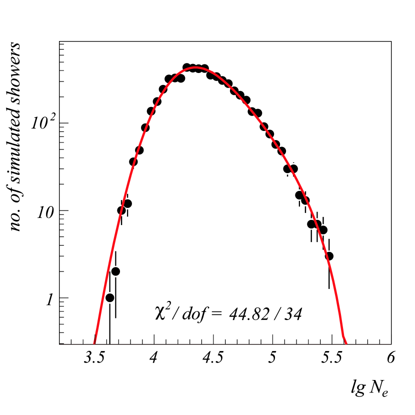
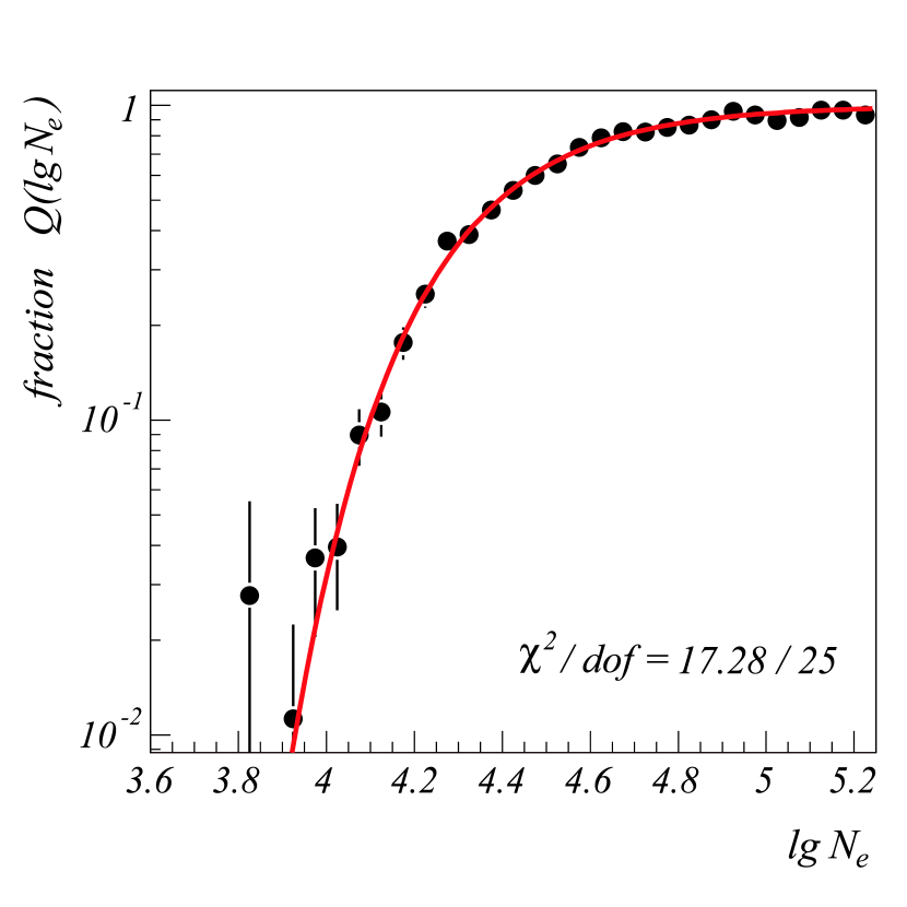
To determine the free parameters of Eq. (7) it is more practicable to determine first the parameters of Eq. (4) via a fit to the electron size distribution and afterwards the muon parameters of Eq. (5) by fitting the truncated muon number distribution. The form of the latter one can be described using Eq. (7) by

$$P(\lg N_{\mu}^{tr}|\lg E)=\int_{-\infty}^{+\infty}\,\frac{P(\lg N_{e},\lg N_{\mu}^{tr}|\lg E)}{d\lg N_{e}}\,d\lg N_{e}.$$ (8)

Figure 4: Left: Distribution of muon number for proton induced showers (0.5 PeV, QGSJet), together with a fit according to Eq. (8). Right: $\lg N_{e}-\lg N_{\mu}^{tr}$ distribution of simulated showers (proton, 0.5 PeV, QGSJet) and the corresponding parameterization.

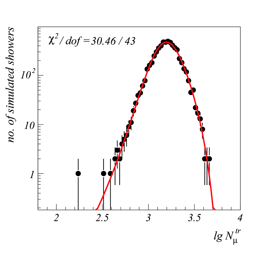
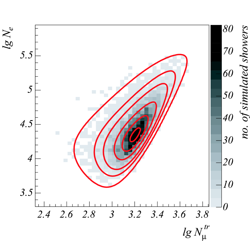
As examples, some distributions for fixed primary energy and the corresponding fits are illustrated in Fig. 3 and Fig. 4.

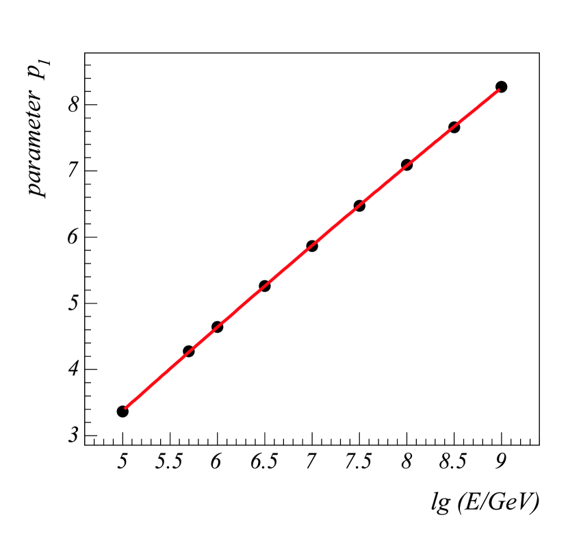
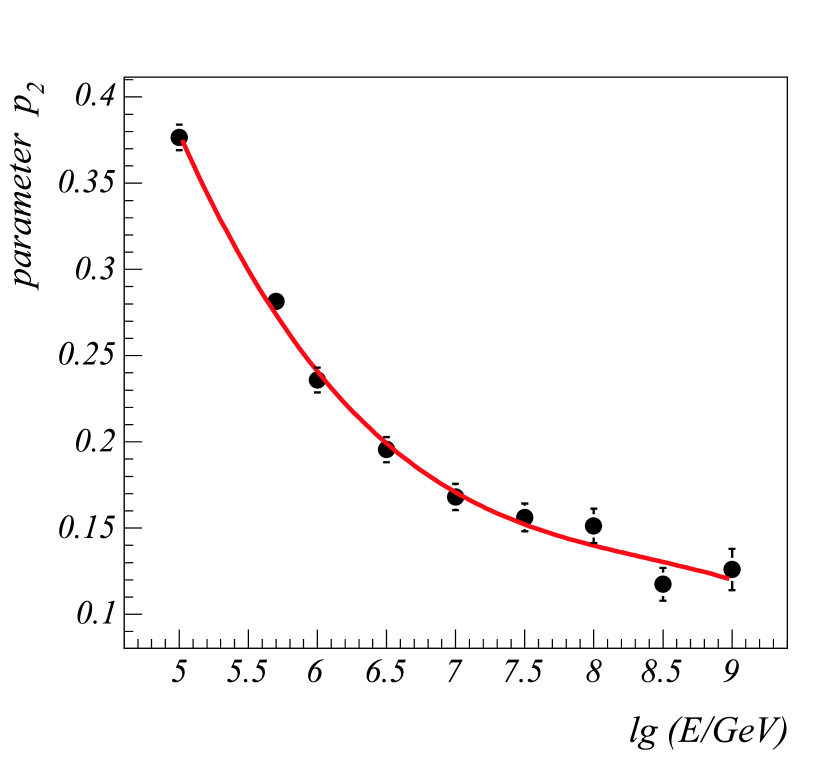
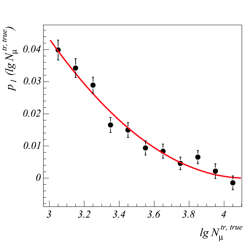
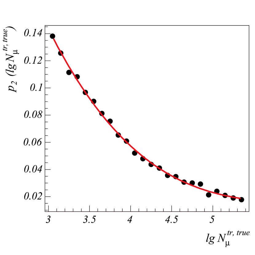
Investigation of the energy dependence of the various parameters showed that for each primary species the parameters $p_{3}$, $p_{5}$, $p_{7}$, $c_{1}$, and $c_{2}$ can be treated as energy independent. Furthermore, for each primary particle type the same values of $p_{4}$ can be used which indicates that the electron number at shower maximum is almost independent of primary mass. The energy dependence of the remaining five parameters is interpolated using polynomials. As an example, the parameters $p_{1}$ and $p_{2}$ for proton induced showers (QGSJet simulations) are displayed in Fig. 5.

Figure 5: Interpolated energy dependence of parameters $p_{1}$ and $p_{2}$ of Eq. (4) for the case of proton induced showers (QGSJet simulations).

4.3 Properties of the reconstruction

For the investigation of the reconstruction properties, the set of fully simulated (no thinning) CORSIKA showers is used, including a GEANT based simulation of the KASCADE experiment. In these detector simulations all properties of the detectors and the electronics are accounted for. The reliability of the simulations was checked independently e.g. by comparison between simulated and measured single muon spectra recorded by the array detectors. The output of the simulations has the same data structure as measured events. Therefore, simulated and measured showers are indistinguishable for the reconstruction process and can be treated with the usual KASCADE reconstruction algorithms.

4.3.1 Estimate of $\epsilon_{A}$

Although the data range for the following analysis is chosen in a way to minimize influences from possible efficiency variations, it is useful to parametrize the combined trigger and reconstruction efficiencies for the calculation of the response matrix elements. Details of trigger and reconstruction efficiencies can be found in [15]. Since the number of fired detectors depends, to very good approximation, on electron shower size only, the trigger efficiency can be well approximated by an integrated Gaussian distribution, depending only on $\lg N_{e}^{true}$.
The reconstruction of a measured shower is only successful if both, electron and muon number, can be determined. The probability of a successful reconstruction depends on the muon number only, as the determination of $N_{e}$ is possible for every triggered shower. The combined efficiency $\varepsilon=\varepsilon(N_{e},N_{\mu}^{tr})$ for triggering the measurement and successful reconstruction can be parameterized by the product of two error functions:

$$\varepsilon={\mathrm{erf}}(a)\cdot{\mathrm{erf}}(b)\quad{\mathrm{with}}\quad a=\frac{\lg N_{e}-p_{0}}{p_{1}},\quad b=\frac{\lg N_{\mu}^{tr}-p_{2}}{p_{3}}$$ (9)

For the considered zenith angle range typical values for proton induced showers are $p_{0}=3.75$, $p_{1}=0.16$, $p_{2}=2.32$, and $p_{3}=0.36$. A slight dependence on primary particle type was found for the parameters $p_{0}$ and $p_{1}$. In conclusion, all showers with $\lg N_{e}>4.4$ and $\lg N_{\mu}^{tr}>3.4$ trigger the experiment and are reconstructed successfully, regardless of primary particle type.

4.3.2 Parameterization of $r_{A}$

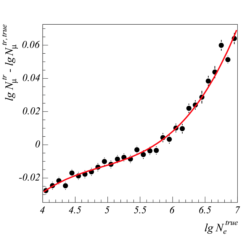
Of further importance for the determination of the response matrix is the difference between reconstructed shower size and its true value. In the case of the electron number the mean value of the difference $\Delta\lg N_{e}=\lg N_{e}-\lg N_{e}^{true}$ shows a dependence on the difference $\lg N_{e}^{true}-\lg N_{\mu}^{tr}$ between true electron and reconstructed truncated muon number. This correlation is displayed in the left part of Fig. 6. This dependence proved to be independent of primary particle type and primary energy and is used for a parameterization of $\Delta\lg N_{e}$ depending on $\lg N_{e}^{true}-\lg N_{\mu}^{tr}$, which defines a correction term $C_{e}$ to be substracted from $\lg N_{e}$.

Figure 6: Left: Difference between reconstructed and true electron number, dependent on the difference $\lg N_{e}^{true}-\lg N_{\mu}^{tr}$. Right: Remaining systematic difference after correction with the relation in the left part of the figure. Simulations were generated using QGSJet.

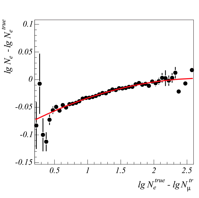
The main reasons for this systematic effect are deviations between the observed lateral distribution and the NKG function used to determine the particle number which has to be integrated over the whole lateral distance range. The size of the systematic difference between true and reconstructed electron number is strongly correlated with the shower age which itself is strongly correlated with the ratio between electron and muon number. A more detailed analysis of these interrelationships will be the topic of a forthcoming paper.

Figure 7: Left: Distribution of $\lg N_{e}-\lg N_{e}^{true}-C_{e}$ for proton induced showers with $4.2<\lg N_{e}^{true}\leq 4.3$ fitted with a Gaussian distribution. Right: Dependence of the width $\sigma$ on the true electron number $\lg N_{e}^{true}$.

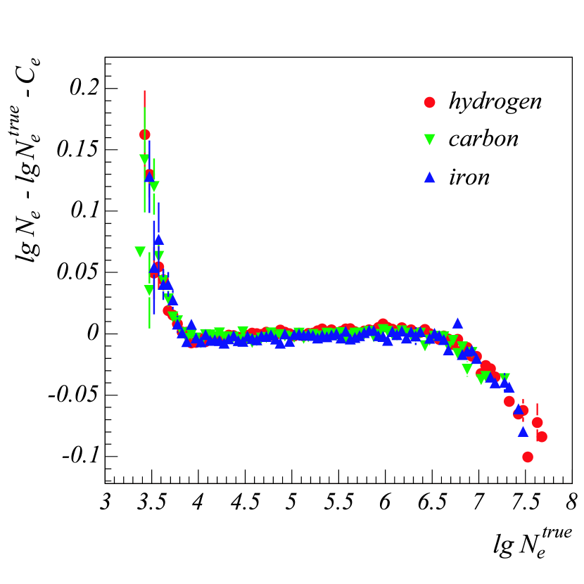
The dependence of the corrected difference $\lg N_{e}-\lg N_{e}^{true}-C_{e}$ on true electron number is displayed in the right part of Fig. 6. The increase towards low values of $\lg N_{e}^{true}$ is due to the combined threshold of measurement and reconstruction, the decrease of $\lg N_{e}-\lg N_{e}^{true}-C_{e}$ towards larger shower sizes reflects saturation effects in the array detectors which influence the quality of the reconstruction. These deviations from the zero line are parameterized and accounted for in the analysis.

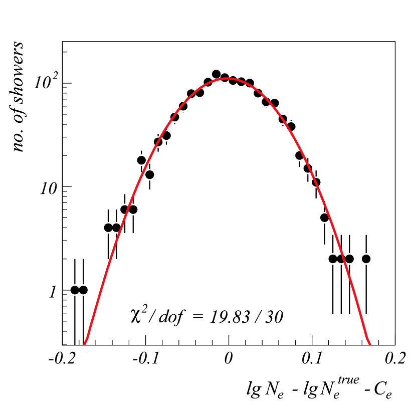
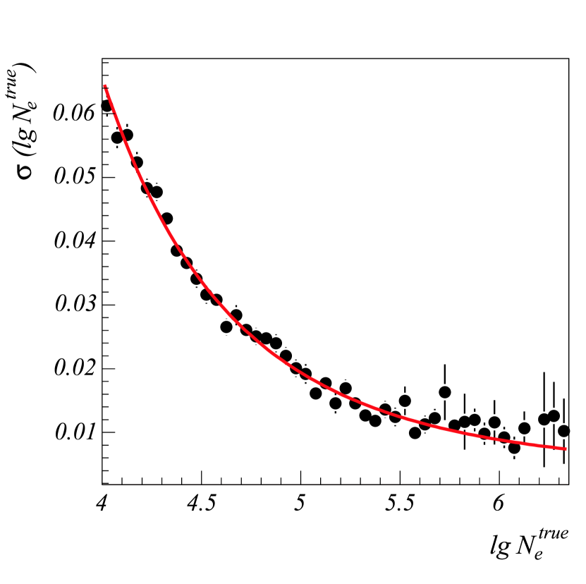
The distribution of $\lg N_{e}-\lg N_{e}^{true}-C_{e}$ for fixed true electron number $\lg N_{e}^{true}$ can be described with good quality by a Gaussian. An example for this is displayed in the left part of Fig. 7. The form and the parameters of this distribution do not depend on primary particle type. The width of the distribution depends on $\lg N_{e}^{true}$ but can be easily parameterized which is displayed in the right part of Fig. 7. The adopted description of the reconstruction systematics and resolution of $\lg N_{e}$ can be integrated into the calculation of the response matrix elements. The influence of resolution effects on the results are small since for the showers used ($\lg N_{e}>4.8$) the resolution is smaller than the bin width in $\lg N_{e}$.

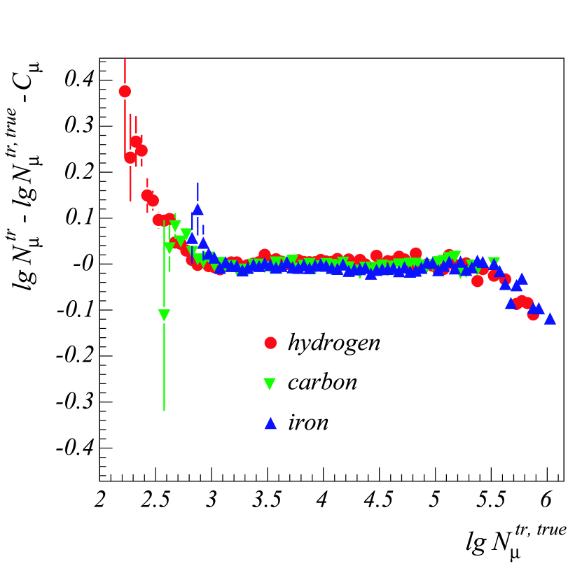
In the case of the truncated muon number a correlation between the difference $\lg N_{\mu}^{tr}-\lg N_{\mu}^{tr,true}$ and the true electron number $\lg N_{e}^{true}$ was found. This correlation, displayed in the left part of Fig. 8, proved also to be nearly independent of primary particle type. Using this correlation for the parameterization of a correction term $C_{\mu}$ any dependence of $\lg N_{\mu}^{tr}-\lg N_{\mu}^{tr,true}$ on $\lg N_{\mu}^{tr}$ nearly vanishes. The mean values of $\lg N_{\mu}^{tr}-\lg N_{\mu}^{tr,true}-C_{\mu}$ versus muon number $\lg N_{\mu}^{tr,true}$ are displayed in the right part of Fig. 8. Deviations from the zero line for small and large values of the muon number have similar reasons as in the case of $\lg N_{e}$ and are accounted for.

Figure 8: Left: Relation between $\lg N_{\mu}^{tr}-\lg N_{\mu}^{tr,true}$ and $\lg N_{e}^{true}$ used for the correction of $\lg N_{\mu}^{tr}$. Right: Remaining systematic differences between reconstructed and true truncated muon number after correction with the relation in the left part of the figure.

Figure 9: Distribution and fit of $\lg N_{\mu}^{tr}-\lg N_{\mu}^{tr,true}-C_{\mu}$ for showers with $3.6<\lg N_{\mu}^{tr,true}\leq 3.7$ (left) and $4.2<\lg N_{\mu}^{tr,true}\leq 4.3$ (right).

Figure 10: Dependence of parameters $p_{1}$ (left) and $p_{2}$ (right) of Eq. (10) on the true muon number $\lg N_{\mu}^{tr,true}$.

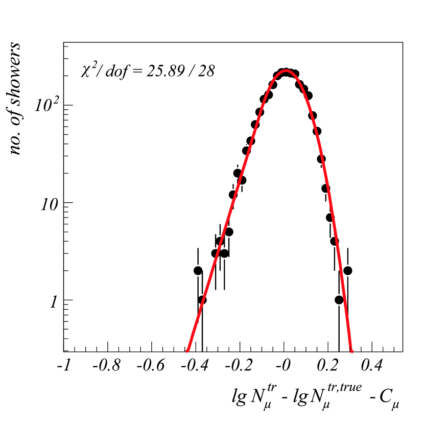
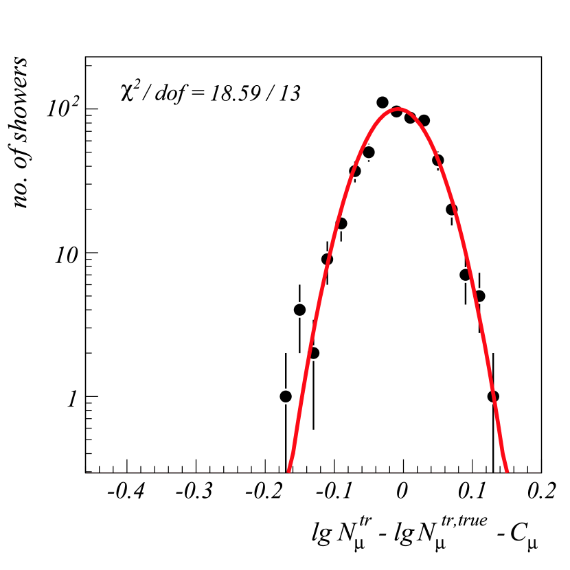
In contrast to the case of the electron number the distribution of $\lg N_{\mu}^{tr}-\lg N_{\mu}^{tr,true}-C_{\mu}$ is asymmetric for smaller values of $\lg N_{\mu}^{tr,true}$ but becomes more and more symmetric with increasing $\lg N_{\mu}^{tr,true}$. For values $\lg N_{\mu}^{tr,true}>4$ the distribution can be described again by a Gaussian. In Fig. 9 these distributions are displayed for two narrow intervals of $\lg N_{\mu}^{tr,true}$. In order to describe the asymmetric distribution the following functional form was used

$$r(x)=\bigg{\{}\begin{array}[]{ll}c_{1}\cdot e^{-\frac{(x-p_{1})^{2}}{2\cdot p_{2}^{2}}}&\quad x>p_{1}-\frac{p_{2}^{2}}{p_{3}}\\ c_{1}c_{2}\cdot e^{\frac{x}{p_{3}}}&\quad x\leq p_{1}-\frac{p_{2}^{2}}{p_{3}}\end{array}$$ (10)

with the factor $c_{2}$ as a normalization constant. The value of $p_{1}$ tends to zero with increasing $\lg N_{\mu}^{tr,true}$. The dependence of $p_{1}$ and $p_{2}$, which can be considered as a measure for the resolution of the muon number determination, on the true muon number are displayed in Fig. 10.

5 Solving the matrix equation

5.1 Application of unfolding methods

From a purely mathematical point of view, solving the matrix equation Eq. (3), only requires a simple inversion of the matrix ${\bf R^{-1}}$. However, a closer inspection of this matrix shows, that it is close to singularity and Eq. (3) states an ill-conditioned problem. Therefore, a direct inversion would give meaningless results.

The reason for the poor condition of the response matrix is closely related to the properties of shower fluctuations. Since for different primary particles the corresponding distributions overlap to a large extent, the discrimination between these particles gets more and more difficult with increasing number of particle types. In the extreme case of very similar particles, like for example nitrogen and oxygen, the corresponding matrix elements would coincide inside the computational accuracy for a reasonable binning of the data. In this case ${\bf R}$ is singular, and an inversion impossible. Therefore, the number of considered particle types has to be restricted.

Another reason lies in the steeply falling primary spectrum. Due to their broad shower fluctuations low energy primary particles may be registered at high electron and muon numbers. Although the probabilities for this are very small this may be compensated by their high flux. This is reflected by a few very small matrix elements (in the order of $10^{-5}$ and smaller). As a result, nearly identical rows and columns consisting of very small values are present in ${\bf R}$ even when only one primary particle type is considered. Again, this leeds to a nearly singular matrix. In addition, also many small off-diagonal elements are introduced in the response matrix which are sensitive to rounding errors.

Altogether, the response matrix ${\bf R}$ exhibits nearly identical rows and columns and many small off-diagonal elements. In such case, inversion of a matrix is in general an ineffective strategy, and one has to rely on methods which approximate the solution avoiding the problems inherent to matrix inversion. One class of methods especially suited for the determination of approximate solutions of ill-conditioned matrix and integral equations are so-called unfolding or deconvolution techniques. For this there exist many different algorithms, each one with its own systematic properties. To get a measure for the size of the systematic errors caused by the unfolding three different methods are used in the present analysis. These are the Gold algorithm [25], unfolding based on the Bayesian theorem [26] and an entropy based unfolding method [27]. Characteristic of these procedures is the generation of only non-negative solutions. Properties of these methods and details about their application are briefly presented in Appendix A.2.

5.2 Considered primary elements

For unfolding techniques to be applicable the matrix equation (3) has to exhibit a minimum degree of stability for the algorithms to provide meaningful solutions. This stability is characterized by the condition number of the response matrix, which is strongly influenced by the number of primary particle types included in the analysis. One is restricted to a maximum number of elements since otherwise this would lead to a singular matrix. The relevant quantity here is the condition number defined by the ratio of the biggest to the smallest singular value of a matrix. The larger its value, the poorer is the condition of the matrix. Acceptable values are in the range of $10^{6}$ to $10^{7}$, depending on the the specific problem.

To find maximum number of particle types, the number was varied, and in each case an unfolding procedure performed. For this investigations results of QGSJet 01 based simulations were used. The quality of the results was judged by means of a $\chi^{2}$-comparison with the measured data (see section 8.2 or 8.3 for details). To determine the condition number of the corresponding matrices a singular value decomposition was performed. For the use of only two primaries (H and Fe) a $\chi^{2}$ per degree of freedom of 245 was achieved, for three particles (H, C, Fe) a value of 35, for four particles a value of 3.3 in the case of H, He, C, and Fe, and 2.5 for the use of H, He, C and Si, respectively. For five elements (H, He, C, Si, Fe) a value of 2.38 for $\chi^{2}$ per degree of freedom was found. At the same time the condition number increases from $2.3\cdot 10^{5}$ (H, Fe) to $1.7\cdot 10^{6}$ (H, C, Fe) and $4\cdot 10^{6}$ for four primaries up to $8.5\cdot 10^{6}$ in the case of H, He, C, Si and Fe. In addition, a significant increase in the statistical uncertainty of the solution with the transition from four to five primaries was observed.

Due to the already large condition number in the case of five elements and only small improvement in the description of the data by the solution, finally five primary particle types are adopted for the analysis. These are hydrogen (protons), helium, carbon, silicon, and iron. The spectra of proton and helium will describe the energy spectra of single elements, whereas the three other types represent elemental groups only, carbon essentially the CNO-group, silicon the intermediate, and iron the heavy elements. Furthermore, it is not possible to specify from which elements of these groups the resulting energy spectra stem.

6 Monte Carlo tests

Before applying any of the unfolding algorithms to measured data it has to be tested if the method is suited for the actual problem. In order to get an estimate of the capabilities and sensitivity of an algorithm it is tested in an “ideal environment”. According to an assumed energy spectrum for each primary particle type energy values are randomly chosen. Electron and muon numbers for each energy value are generated by Monte Carlo techniques, using the parametrized shower fluctuations and reconstruction properties, and a two-dimensional shower size spectrum, in range and binning identical with the measured one, is filled. The generated data correspond to approximately one third of the KASCADE data used. This artifical data histogram is input for the unfolding algorithms.

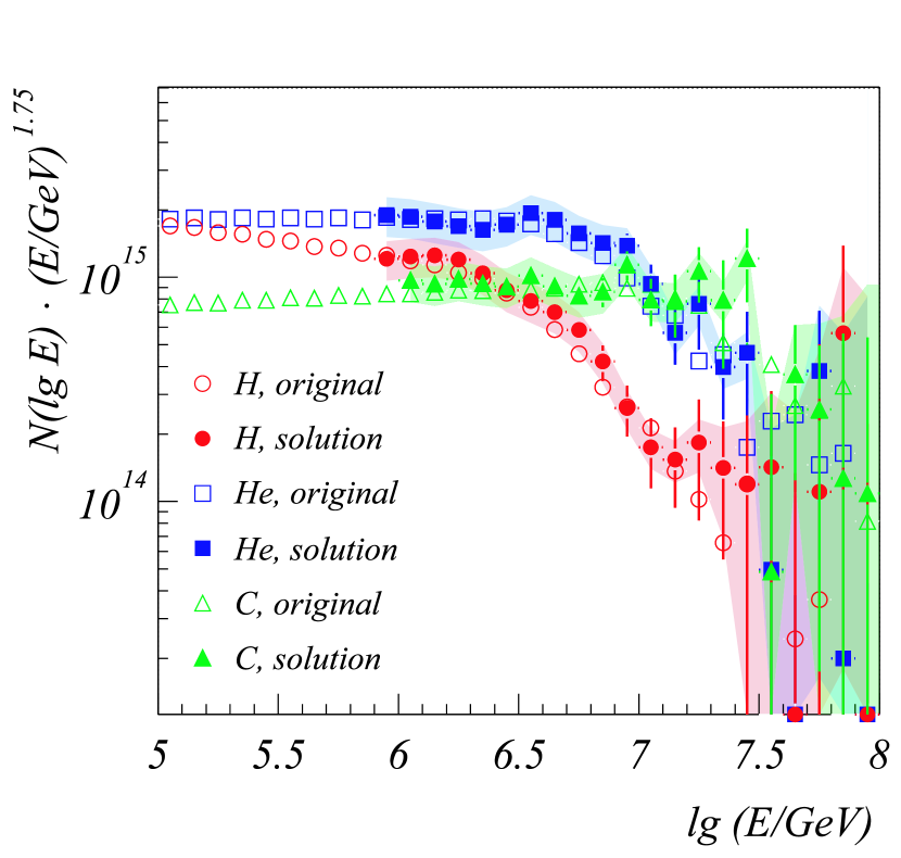
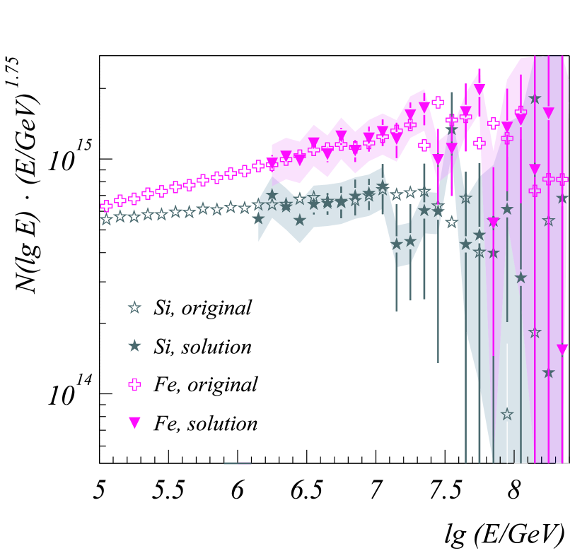
The test procedure was carried out for different assumptions of the individual energy spectra. Considered cases include knee features in each spectrum at different energies, knee features at the same primary energy, knee features only in some of the elemental spectra, and only simple power laws (no knees at all). In all cases similar good results were achieved. In the following the test procedure and its results are presented for the example of a rigidity dependent knee. The assumed energy spectra follow a power law exhibiting a knee with the individual knee positions chosen to be proportional to the particle charges. All three unfolding methods yielded good and comparable results. As an example, the results of the Gold algorithm is presented here which is preferred because of its speed and robustness. A comparison between the results of the different unfolding algorithms is presented in section 7.1 and in Fig. 12 for the unfolding of the KASCADE data using QGSJet simulations. The ”true” spectra of proton, helium, carbon, silicon, and iron are depicted by the open symbols in Fig. 11. Flux values and spectral indices below the knee are based on the compilation of [28].

To obtain reliable results, some criterion to stop the iteration is required. For the determination of the adequate number of iteration steps the weighted mean squared error (WMSE) and the relative variance of the bias (RBS) are used. These quantities are defined by

$${\mathrm{WMSE}}=\frac{1}{m}\sum_{i=1}^{m}\frac{\sigma_{X,i}^{2}+b_{i}^{2}}{\tilde{X}_{i}}\quad{\mathrm{and}}\quad{\mathrm{RBS}}=\frac{1}{m}\sum_{i=1}^{m}\frac{b_{i}^{2}}{\sigma_{b,i}^{2}},$$ (11)

where $m$ is the dimension of the solution, $\tilde{X}_{i}$ the value of the $i$th element of the solution vector $\vec{X}$ and $\sigma_{X,i}^{2}$ its variance; $b_{i}$ is the systematic bias from the true value and $\sigma_{b,i}$ the statistical uncertainty of this bias. Details about their use in unfolding analyses can be found in [29]. For the determination of the WMSE and RBS a bootstrap method is used. The solution of the current iteration step serves as model for the generation of a set of Monte Carlo data which are deconvoluted. The obtained solution set is compared to the input spectra, i.e. the original solution. This method proved to work well for the estimation of the WMSE and RBS but provides a good estimate of the absolute value of the average systematic uncertainties only, and not for their sign.

The result of the unfolding is shown in Fig. 11 for the Gold method. The open symbols correspond to the original “true” spectra, filled symbols represent the solution of the unfolding procedure. The left part of the figure displays the spectra of protons, helium, and carbon, the spectra of silicon and iron are shown in the right part. Error bars represent statistical errors whereas systematic uncertainties are shown as shaded bands. Statistical errors are due to the limited number of simulated data and are estimated by repeating the unfolding with different sets. Systematic uncertainties are estimated by comparison of the mean value of the set of results with the values of the original “true” spectra. These systematic uncertainties are mainly due to the uncertainty in terminating the iteration and the value of the regularization parameter, respectively. For all three unfolding methods this uncertainty is of order 15% for low energies, i.e. high fluxes. The strong increase of the systematic uncertainties at higher energies is due to the low fluxes and hence small number of showers. Since the considered algorithms are designed to generate only non-negative solutions they tend to introduce an additional bias in the case of small number of events. This bias gets significantly large for energies with less than $\approx 30$ events per bin.

As can be seen in Fig. 11, the spectral features of the original spectra, like knee position and spectral index, are well reproduced within the statistical and systematic uncertainties. The artifical “wobbling” at low energies can be identified as a systematic relic of the unfolding procedure. Assuming a smooth behaviour of the original spectrum this yields an independent estimate for the size of the systematic uncertainties, again of order 15%. For the determination of the spectral shapes and the spectral indices these systematic effects have to be considered. Altogether, it can be concluded that the proposed analysis technique is applicable to the problem of unfolding the two-dimensional air shower size spectrum with five primary mass groups.

Figure 11: Unfolding results (filled symbols) for the energy spectra of H, He and C (left panel) and Si and Fe (right panel) together with the original ”true” spectra (open symbols). The shaded bands are an estimate of the systematic uncertainties due to the applied unfolding method, in this case the Gold algorithm.

7 Results

7.1 Results based on QGSJet 01

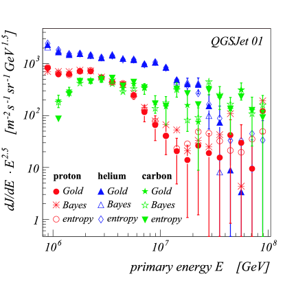
All three unfolding procedures mentioned above were used in order to cross-check the solution. The result for the energy spectra of the light element groups (H, He, C) are shown in Fig. 12 for the three methods. The different unfolding results agree very well with each other. The same holds also for the heavy groups and also for the results based on SIBYLL simulations, presented in section 7.2. Therefore, in the following only the results using the Gold algorithm will be discussed which showed the highest speed and robustness among the applied methods.

Figure 12: Results using QGSJet hypothesis for the elements H, He, C and for three different unfolding algorithms. For reason of clarity statistcal error bars are displayed for the results of the Gold algorithm only.

Figure 13: Different extrapolations of the $\lg N_{e}$-distribution for 0.5 PeV proton induced showers (QGSJet 01).

In addition to the statistical uncertainties due to the limited number of measured showers and the systematic uncertainties due to the unfolding algorithm, two additional sources of uncertainties have to be considered.

First, the number of simulated showers is limited, giving rise to further statistical uncertainties of the fit parameters. To estimate this influence, each parameter of Eq. (7) is varied randomly within its error distribution. For each new set of parameters the energy dependence is interpolated and new response matrices are calculated. The unfolding is repeated with each set of response matrices and the spread of the individual fluxes determined. This additional statistical error is already included in the error bars in Fig. 12.

Figure 14: Unfolded energy spectra for H, He, C (left panel) and Si, Fe (right panel) based on QGSJet simulations. The shaded bands are an estimate of the systematic uncertainties due to the used parametrizations and the applied unfolding method (Gold algorithm).

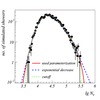
Second, the form of the tails of the shower size distributions is not known. Fig. 13 shows an example of the $\lg N_{e}$–distribution for showers induced by 0.5 PeV protons. Besides the parameterization used, two different extrapolations are displayed, the first one with sharp cutoffs at the edges of the distribution, the second one with an exponential decrease up to higher and lower values of $\lg N_{e}$. Within the statistics of the simulations each of these functions describes the distribution equally well. The influence of these tails on the shower size spectra and the unfolding result may be quite important because of the steeply falling primary energy spectra. The displayed parameterizations in Fig. 13 can be regarded as extreme assumptions and it has been investigated that the corresponding unfolding results form an upper and lower bound for the spectra. This range can be considered as an estimate for the systematic uncertainty due to the unknown shape of the distribution tails. It should be mentioned that the size of this systematic uncertainty should, according to simulations, be considerably reduced for observations close to shower maximum (e.g. around 5000 m a.s.l.).

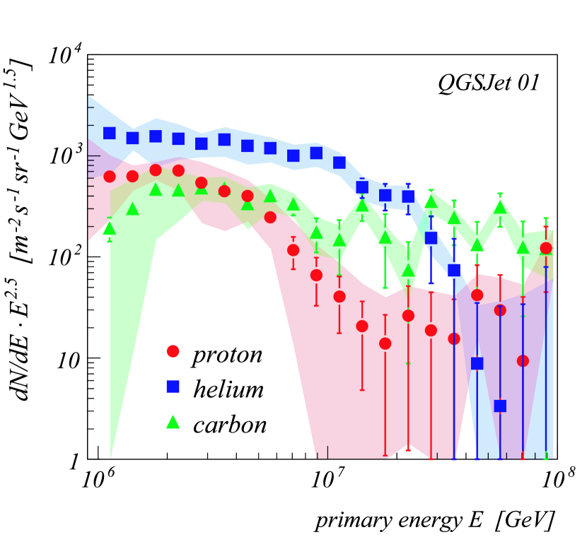
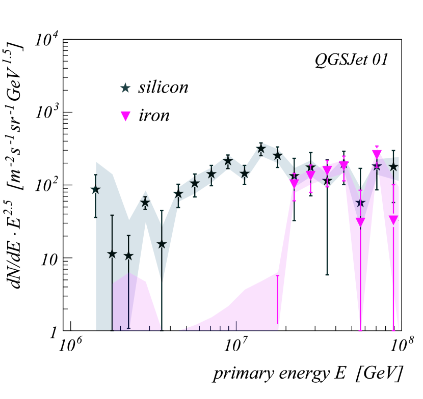
In Fig. 14 the unfolding result is displayed together with the estimate of the total systematic uncertainty, shown as shaded bands. For low energies, the dominant contribution to the systematic uncertainty is due to the tails of the distributions.

Below the knee helium is the most abundant element, followed by protons and carbon. The energy spectra of both proton and helium show a knee-like feature whereas for carbon no knee structure is visible. The spectra of the heavier elements look rather unexpected, especially in the case of iron. For energies below 10 PeV practically no iron is present, above 20 PeV it dominates the cosmic ray spectrum together with silicon.

7.2 Results based on SIBYLL 2.1

The outcome of the unfolding using CORSIKA/SIBYLL/GHEISHA for calculation of the response matrices is presented in Fig. 15 for the Gold algorithm and five particle types.

Figure 15: Unfolded energy spectra for H, He, C (left panel) and Si, Fe (right panel) based on SIBYLL simulations. The shaded bands are estimates of the systematic uncertainties due to the used parameterizations and the applied unfolding method (Gold algorithm).

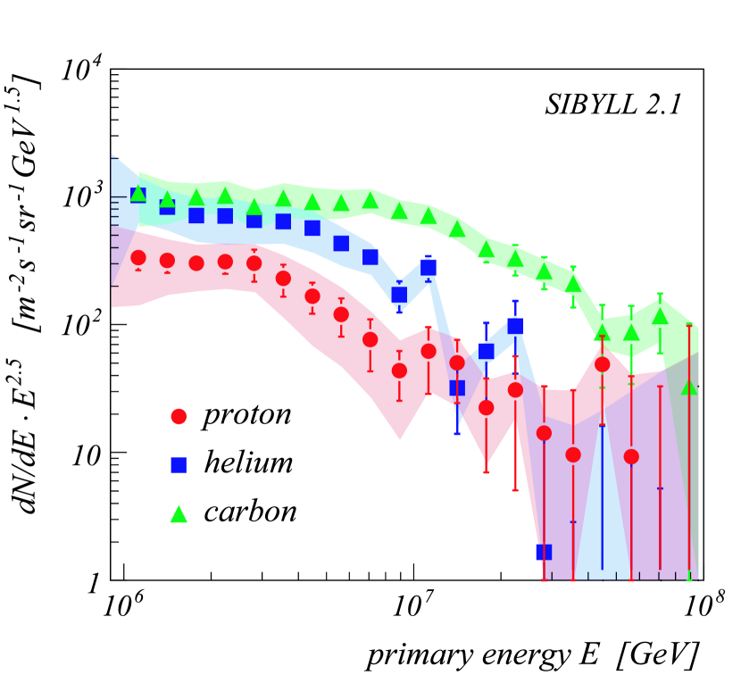
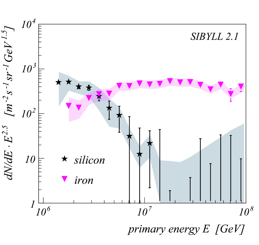
As in the case of the QGSJet analysis the different unfolding methods give essentially equal results. The estimated total systematic uncertainties at lower energies are slightly smaller than for the QGSJet based results due to a better description of the measured data in the corresponding data range, which will be discussed in section 8.3. Each of the spectra of the light groups (proton, helium and CNO) shows a knee-like feature. The position of the individual knees is shifted to higher energies with increasing atomic number. In contrast to the QGSJet results, carbon is the most abundant element at energies around 1-2 PeV but helium is again more abundant than hydrogen.
The spectrum of silicon looks rather unexpected, exhibiting a knee-like structure at around 3 PeV and decreasing very steeply above. Contrary to silicon, the iron spectrum looks very flat in this representation with a slight change of index to $\gamma\approx-2.5$ above 10 PeV. This behaviour of the heavy group spectra will be discussed in section 8.3.

8 Discussion

8.1 All particle energy spectrum

By summing up the five mass group spectra the all particle spectrum is obtained. It is displayed in Fig. 16 for both solutions. The estimated statistical uncertainties are shown by the error bars, the shaded band represents the estimated systematic uncertainty, due to the applied method (Gold algorithm) and the parameterization of the tails of the shower size distribution, for the QGSJet results only. The corresponding band for the SIBYLL solution is of same size and omitted here for reasons of clarity. Tabulated values of the spectra are given in Appendix B.

Figure 16: Result for the all particle energy spectrum using QGSJet and SIBYLL simulations in the analysis. The shaded band represents the estimated systematic uncertainties for the QGSJet solution which are of the same order for the SIBYLL solution. For reasons of clarity only the QGSJet band is displayed.

Figure 17: All particle spectrum for the QGSJet 01 based analysis in comparison with results from RUNJOB [31], JACEE [32], Proton-3 [33], EAS-TOP [34], Tibet [35], HEGRA [36], Akeno [37], CASA-MIA [38], CASA-BLANCA [39], and DICE [40].

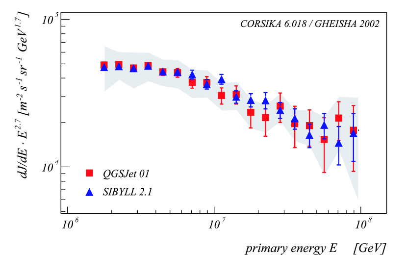
The knee is clearly visible for both cases. The spectrum is fitted with the expression [30]

$$\frac{dJ(E)}{dE}=p_{0}\cdot E^{p_{2}}\left(1+\left(\frac{E}{p_{1}}\right)^{p_{4}}\right)^{(p_{3}-p_{2})/p_{4}},$$ (12)

where $p_{1}$ corresponds to the knee position, $p_{2}$ and $p_{3}$ are the spectral indices below and above the knee, and $p_{4}$ is a parameter describing the sharpness of the knee. In the case of the QGSJet 01 solution for the knee position a value of $4.0\pm 0.8$ PeV and for the spectral indices $-2.70\pm 0.01$ and $-3.10\pm 0.07$ were obtained. For the SIBYLL solution the corresponding values are $5.7\pm 1.6$ PeV, $-2.70\pm 0.06$, and $-3.14\pm 0.06$. In both cases, the fit is insensitive to the value of $p_{4}$ which was therefore fixed to a value of 4. The $\chi^{2}$ per degree of freedom is 0.35 in the QGSJet case, and 0.42 for the SIBYLL solution. Within statistical uncertainties the results for the two interaction models coincide. It should be stressed that although the band of systematic uncertainties might suggest the possibility of a spectrum without a knee, each of the spectra defining this band exhibits a knee at around 5 PeV.

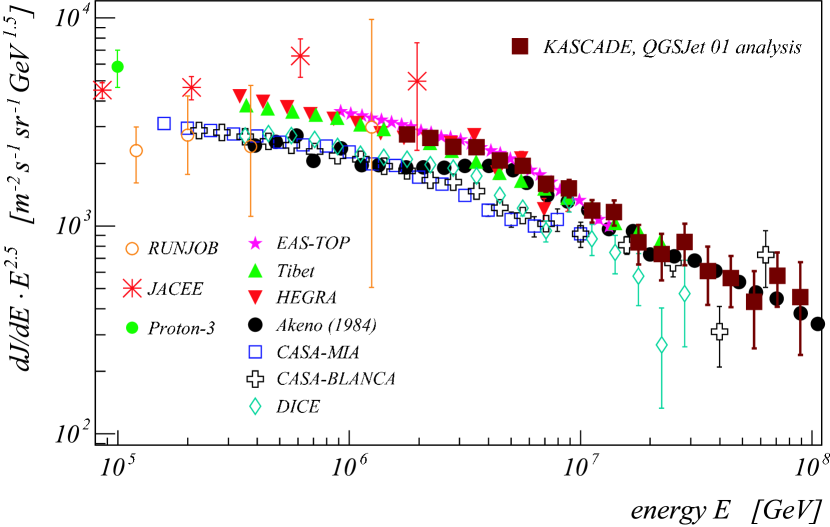
This result is essentially independent of the interaction models used and in good agreement with results from other experiments. In Fig. 17 the QGSJet based results are displayed together with results from some other experiments. Concerning the flux at the knee and the knee position a very good agreement is especially reached with the HEGRA and the EAS-TOP experiments.

8.2 Description of data – QGSJet based analysis

To judge on the properties and the quality of the solution a vector $\vec{Y}_{con}$ is “constructed“ by forward folding of the solution according to Eq. (3) and a $\chi^{2}$ test is performed. This results in a value of $\chi^{2}_{dof}=2.38$. The individual contributions $\chi^{2}_{i}$ of interval $i$ to this value are displayed in Fig. 18 as a twodimensional distribution. It is obvious that the obtained solution is not able to describe the data satisfactorily.

Figure 18: Distribution of the individual $\chi^{2}_{i}$ in the data range for the QGSJet solution.

Figure 19: Comparison of measured data with the QGSJet based solution. Left: Electron size distribution for $4<\lg N_{\mu}^{tr}<4.1$. Right: Electron size distribution for $4.85<\lg N_{\mu}^{tr}<4.95$.

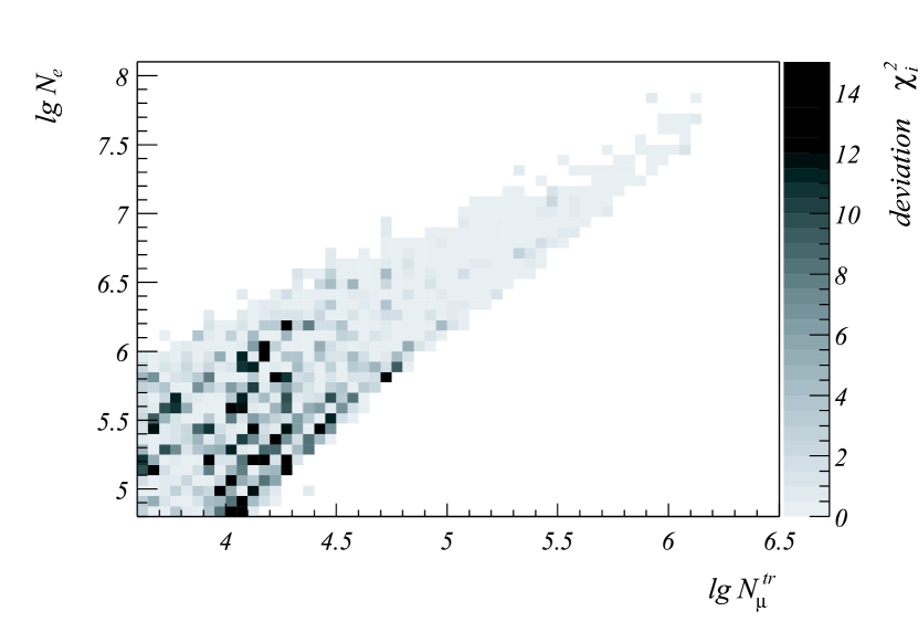
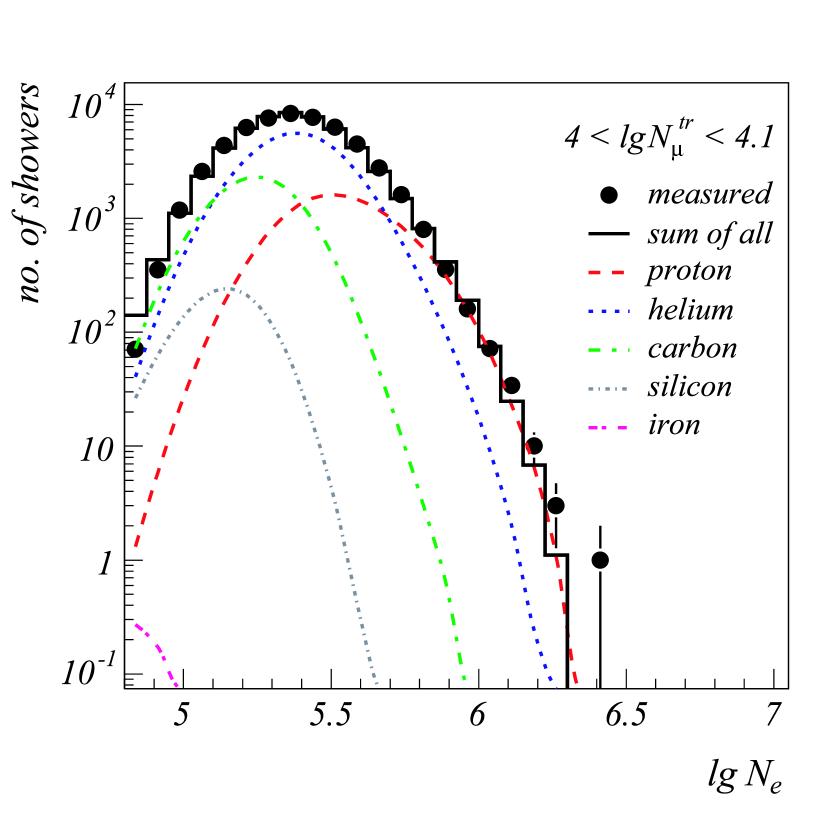
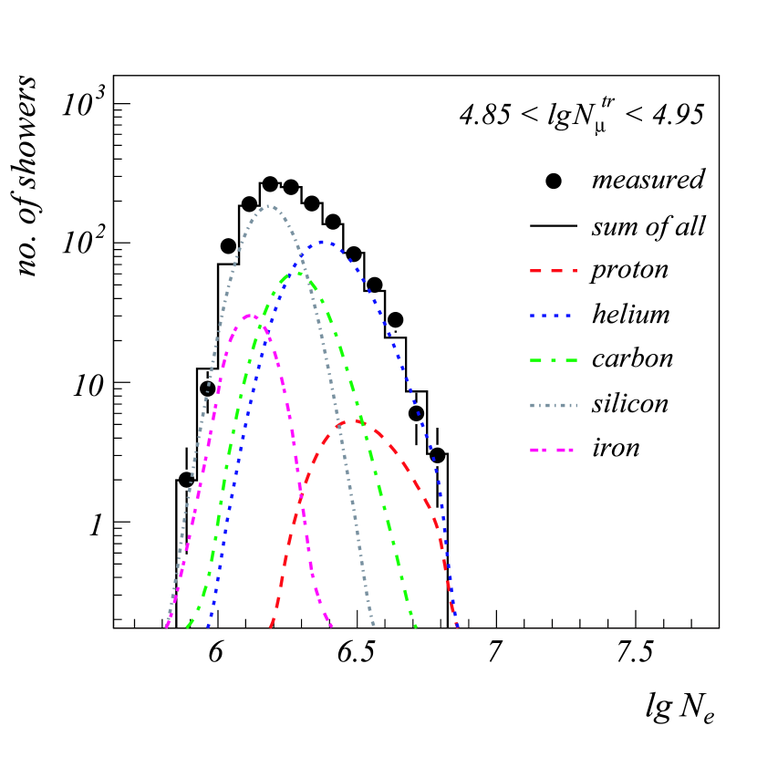
The bulk of the deviations between measured and constructed data is concentrated in the lower part of the measurement range, i.e. at low energies, with a slight concentration in the region of small electron numbers (for fixed muon number), i.e. showers induced by heavy primaries. For higher energies (large shower sizes) the description of the data is quite well within the statistical uncertainties.

To clarify the nature of these deviations, it is instructive to look at the $\lg N_{e}$-distribution for given $\lg N_{\mu}^{tr}$ bins. Fig. 19 displays the measured distributions (points) for different $\lg N_{\mu}^{tr}$ bins together with the resulting distributions of the forward folding (histogram). In addition, the contribution of the different primary types are shown by smooth curves. As can be seen, a large contribution of showers induced by light elements is needed for small muon number bins to describe the right tail of the distribution (large electron numbers). As a consequence, no iron showers are needed for the description of the left-hand tail of the distribution. Even with practically no iron present at all there are still more showers with $\lg N_{e}<5$ calculated than measured. 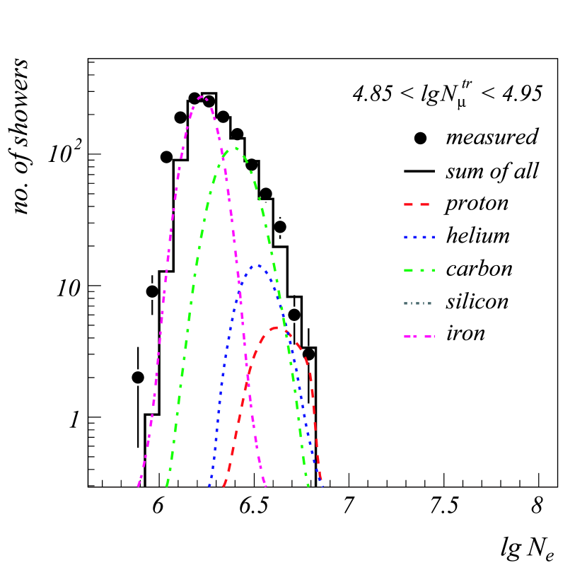The situation improves for higher energies (large muon numbers). First, the description of the distribution is better; second, now iron is also required to describe the measured electron sizes. By investigating such figures the reason for the negligible iron flux at low energies for the QGSJet result can be understood. Investigations of the $\lg N_{\mu}^{tr}$-distributions for different $\lg N_{e}$ bins yield corresponding results.
To summarize, showers generated using QGSJet seem to predict too many muons or too few electrons at low energies than required by the data.

8.3 Description of data – SIBYLL based analysis

A similar comparison was performed using results based on the SIBYLL model. An overall value for $\chi^{2}_{dof}$ of 2.46 was obtained, being quite similar to the QGSJet case. Again the solution is not capable to describe the measured data in the complete region of measurement. The distribution of individual $\chi^{2}_{i}$, displayed in Fig. 20, is very different compared to the QGSJet based solution (Fig. 18). The bulk of the deviations is concentrated at medium to high $\lg N_{\mu}^{tr}$ and small $\lg N_{e}$, i.e. in the region of heavy primaries with higher energies. Other than with the QGSJet solution, only small deviations occur at low energies.

Figure 20: Distribution of the individual $\chi^{2}_{i}$ in the data range for the SIBYLL solution.

Figure 21: Comparison of measured data with the SIBYLL based solution. Left: Electron size distribution for $4<\lg N_{\mu}^{tr}<4.1$. Right: Electron size distribution for $4.85<\lg N_{\mu}^{tr}<4.95$.

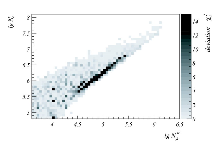
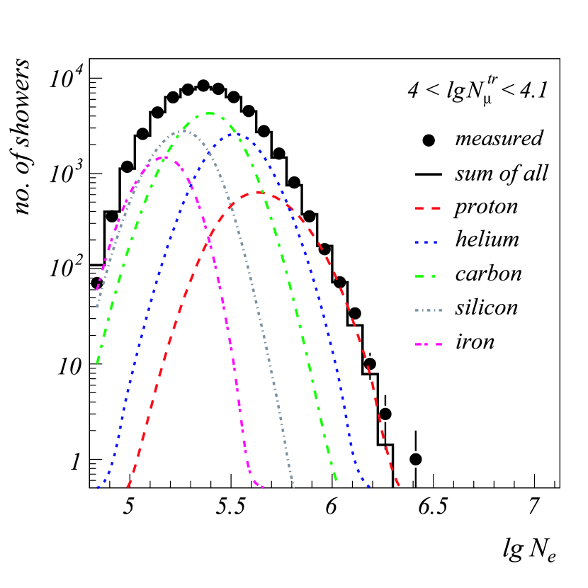
In Fig. 21 the measured electron size distributions together with the constructed distributions are displayed for the same $\lg N_{\mu}^{tr}$ bins as in Fig. 19. The description of the $\lg N_{e}$-distribution for low $\lg N_{\mu}^{tr}$ bins is much better than for the QGSJet based result, only small deviations are found. Since the maximum of the $\lg N_{e}$-distribution for carbon induced showers nearly coincides with that of the measured distribution, a high abundances of this mass group is found in case of the SIBYLL based solution. The good description of the low energy data range by the SIBYLL based simulations is also the reason for the smaller systematic uncertainties in Fig. 15 at lower energies when compared to the QGSJet results. These uncertainties are dominated by the unknown shape of the tails of the shower fluctuations $s_{A}$ and reflect the stability of the solution against disturbances of the response matrix like changes of the distribution tails. This stability is highest for well described data, resulting in smaller uncertainties.

In contrast, the description in the higher $\lg N_{\mu}^{tr}$ range is much worse than before. This can be seen in the right part of Fig. 21. In particular the left-hand tail of the $\lg N_{e}$-distribution cannot be described using the five assumed particle types. In order to fit the distribution as well as possible the iron contribution has to be raised nearly to the maximum value allowed by the maximum of the observed distribution. On the other hand, the right tail towards higher values of $\lg N_{e}$ can only be described using the lighter elements. As a result, there is no space left for a significant contribution of silicon which explains the sharp decrease in the silicon spectrum in Fig. 15. Whereas the data description at lower energies works quite well, at higher energies showers generated with the SIBYLL model seem to be too electron rich or too muon poor compared to the data. The same conclusion holds when investigating the $\lg N_{\mu}^{tr}$-distribution for different $\lg N_{e}$ bins.

8.4 Some qualitative considerations – open problems

Despite the fact that none of the two hadronic interaction models is able to describe the whole data range consistently, it is possible to get hints, why their predictions do not match the data and how agreement with the data could be improved. In Fig. 22 a part of the two-dimensional size spectrum and in addition some lines of constant intensity (isolines) are drawn. Overlaid are lines representing the energy dependence of the maximum value of the probability distributions $p_{A}(\lg N_{e},\lg N_{\mu}^{tr}|\lg E)$ of Eq. (1), i.e. the most probable pair of the shower size values. These lines of the most probable values are displayed for the primary particles hydrogen (proton) and iron and for the two simulation sets.

Figure 22: Two-dimensional shower size spectrum of $\lg N_{e}$ and $\lg N_{\mu}^{tr}$ together with isolines and lines of the most probable values for proton and iron induced showers for both simulations.

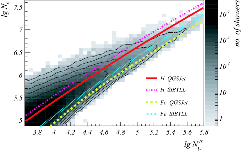
It is noticeable that the lines of the most probable values for the two interaction models are nearly parallel. For SIBYLL simulations these lines are evenly shifted towards larger values of $\lg N_{e}$ and smaller values of $\lg N_{\mu}^{tr}$ with respect to the corresponding lines for QGSJet simulations.

For the SIBYLL based simulations the line of the most probable values of iron showers tends to lie the more in the central region of the data the higher the energy and moves away from the lower edge (small $\lg N_{e}$ for fixed $\lg N_{\mu}^{tr}$) of the data distribution. This lower edge is expected to be dominated by showers induced by heavy elements. Consistent with this relatively large distance to the lower edge are the discrepancies in the description of the measured data by the SIBYLL based results for higher energies (Fig. 21). One way to solve this problem would be a reduction of the predicted electron number in high energy SIBYLL simulations which would result in a decreasing slope of the corresponding lines of the most probable values. Another possibility might be a weaker decrease of shower fluctuations in SIBYLL simulations with increasing energy.

In the case of the QGSJet based solution the description of the data at higher energies is better whereas discrepancies occur at lower energies (see Fig. 19). In the region of small shower sizes no contribution of the heavy component is needed to describe the data. Referring to Fig. 22, one approach would be to shift the lines of the most probable values in the region of smaller shower sizes away from the lower edge of the data distribution. This would mean that more electrons or fewer muons are predicted for showers at low energies. Another possibility could be the reduction of shower fluctuations at lower energies for QGSJet based simulations.

One might argue that the low energy hadronic interaction model could influence the simulations and contribute to the differences. However, when using the FLUKA [41] instead of the GHEISHA code we found almost no changes for the electron and muon shower size distributions. Therefore, FLUKA is not able to improve the situation significantly.

Although these considerations are qualitative they may give some hints for further improvement of hadronic interaction models. Investigations with a toy model which consists of simply shifting the predictions of SIBYLL based simulations towards QGSJet based predictions with increasing energy, resulted in a consistent description of the measured data. (We are aware that this is not a very reasonable procedure.)

8.5 Systematic model uncertainties - the proton spectrum

Figure 23: Results for the proton energy spectrum for both of our analysis together with results from direct (AMS[42], BESS[43], CAPRICE[44], Ryan[45], SOKOL-2 [46], RUNJOB[31], JACEE[32]) and indirect (HEGRA[47], Tibet[48]) measurements.

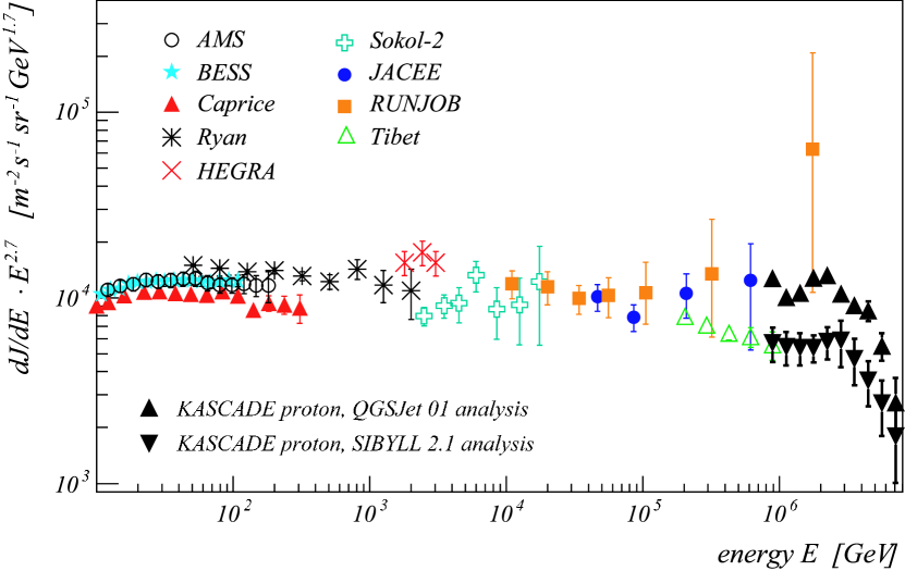
Since neither of the interaction models used in the analysis can describe the measured data consistently the results for the individual element spectra are not fully reliable. However, the difference between the results for the spectrum of one particular particle can serve as an estimate of the systematic uncertainty due to the hadronic interaction models.

To visualize this uncertainty, it is instructive to compare direct and indirect measurements of protons at lower energies with the corresponding spectra of our analyses (Fig. 23). Due to the low abundances of elements lighter than carbon but other than proton and helium the results for proton would give the real spectrum of the single element in the case of correct simulations. Since the elements carbon, silicon, and iron stand for elemental groups, which are loosely defined, a comparison with data from direct measurements is not possible for these heavier elements.

Despite the large difference between our two results they are in good agreement with the extrapolations of those of balloon-borne experiments for the proton spectrum. At present, the statistical uncertainties of direct measurements above $10^{14}$ eV are of the same order of magnitude as the systematic uncertainty of air shower based analyses due to the hadronic interaction models. Further improvement requires a more reliable theoretical description of high energy hadronic interactions.

9 Summary and conclusion

Using the two-dimensional shower size spectrum of electron number $\lg N_{e}$ and muon number $\lg N_{\mu}^{tr}$ measured with KASCADE an analysis was presented yielding energy spectra for five primary mass groups, representing the chemical composition of cosmic rays. For this analysis, air shower simulations with two different high energy hadronic interaction models (QGSJet 01 and SIBYLL 2.1) were used. The reconstructed all particle spectra for both simulation sets coincide within the statistical and systematic uncertainties and are consistent with results from other experiments. The knee is observed at an energy around $\approx 5$ PeV with a change of index $\Delta\gamma\approx 0.4$. The situation differs quite strongly when considering the results of the mass group spectra. Common is the appearence of knee-like features in the spectra of the light elements. For both models the position of the knees in these spectra is shifted towards higher energy with increasing element number. A closer inspection revealed that none of the two interaction models is capable of describing the measured data consistently over the whole measurement range. For the QGSJet based analysis deviations occur at low energies whereas for the SIBYLL based analysis the higher energies are problematic.

Summarizing, it has been demonstrated that unfolding methods are capable to reconstruct energy spectra of individual mass groups from air shower data, in addition to the all particle spectrum. At present, the limiting factors of the analysis are the properties of the high energy interaction models used and not the quality or the understanding of the KASCADE data. The observed discrepancies between simulations and data have to be attributed to the models and may give valuable information for their further improvements.

Appendix A The matrix equation and unfolding methods

A.1 Formulation of the problem as matrix equation

The bin content $N_{i}$ of each cell of the two-dimensional shower size spectrum displayed in Fig. 2 can be written as

$$N_{i}=2\pi A_{s}T_{m}\sum_{A=1}^{N_{A}}\int_{0^{\circ}}^{18^{\circ}}\int_{-\infty}^{+\infty}\frac{dJ_{A}}{d\lg E}\/p_{A}((\lg N_{e},\lg N_{\mu}^{tr})_{i}|\lg E)\frac{1}{2}\sin 2\theta\,d\lg E\,d\theta$$ (13)

with the differential flux $dJ_{A}/d\lg E$ of an element of mass number $A$ and the conditional probability $p_{A}$ describing the probability to measure a shower of primary energy $\lg E$ and primary mass $A$ with shower sizes $(\lg N_{e},\lg N_{\mu}^{tr})_{i}$. For sufficiently large showers, which are only included in the present analysis, measurement time $T_{m}$ and sampling area $A_{s}$ can be treated as constants and no dependence on azimuth angle is present, resulting in the factor $2\pi$.

The probability $p_{A}$ can be expressed as

$$p_{A}=\int_{-\infty}^{+\infty}\int_{-\infty}^{+\infty}s_{A}\epsilon_{A}r_{A}\,d\lg N_{e}^{true}\,d\lg N_{\mu}^{tr,true}$$ (14)

with the primary dependent intrinsic shower fluctuations $s_{A}$, the properties of the reconstruction (resolution and systematic shifts) $r_{A}$ and the combined efficiencies for detection and reconstruction $\epsilon_{A}$.

Simulation studies have shown that at KASCADE efficiencies $\epsilon_{A}$ and reconstruction properties $r_{A}$ do not depend on zenith angle $\theta$ for $\theta<20^{\circ}$. In addition the angular resolution of the KASCADE array in the considered shower size range is better than 0.2^∘, so effects due to limited angular resolution can be savely neglected. Since only showers with $0^{\circ}\leq\theta<18^{\circ}$ are considered, the integration over zenith angle can be incorporated into $s_{A}$. In this sense Eq. 13 can be written as

$$N_{i}=A_{s}T_{m}\Delta\Omega\sum_{A=1}^{N_{A}}\int_{-\infty}^{+\infty}\frac{dJ_{A}}{d\lg E}\/p_{A}((\lg N_{e},\lg N_{\mu}^{tr})_{i}|\lg E)\,d\lg E$$ (15)

with effective solid angle $\Delta\Omega$. The mentioned integration over zenith angle is now included in the shower fluctuations.

Using the abbreviation

$$x_{j}^{A}=A_{s}T_{m}\Delta\Omega\int_{\lg E_{j}}^{\lg E_{j}+\Delta\lg E}\frac{dJ_{A}}{d\lg E}\,d\lg E$$ (16)

the integral can be written as a sum over $n$ energy intervals of width $\Delta\lg E$ with $\lg E_{j}$ denoting the lower bin edges:

$$N_{i}=\sum_{A=1}^{N_{A}}\sum_{j=1}^{n}R_{ij}^{A}\/x_{j}^{A}$$ (17)

Here the matrix element $R_{ij}^{A}$ is defined by

$$R_{ij}^{A}=\displaystyle\frac{\displaystyle\int_{\lg E_{j}}^{\lg E_{j}+\Delta\lg E}\frac{dJ_{A}}{d\lg E}\/p_{A}((\lg N_{e},\lg N_{\mu}^{tr})_{i}|\lg E)\,d\lg E}{\displaystyle\int_{\lg E_{j}}^{\lg E_{j}+\Delta\lg E}\frac{dJ_{A}}{d\lg E}\,d\lg E}.$$ (18)

For small bin width $\Delta\lg E$ the value of the matrix elements $R_{ij}^{A}$ are not sensitive to the correct shape of the differential energy spectra $dJ_{A}/d\lg E$. A decoupling between the matrix element $R_{ij}^{A}$ and the fluxes $dJ_{A}/d\lg E$ is then achieved. In the present analysis a bin width of $\Delta\lg E=0.1$ is chosen which turns out to be sufficiently small.

Introducing the $m$-dimensional data vector $\vec{Y}$ which contains the $m$ cell contents $N_{i}$ of the two-dimensional shower size spectrum, the relation between data and energy spectra can be written as

$$\vec{Y}=\sum_{A=1}^{N_{A}}{\bf R^{A}}\vec{X^{A}}\quad{\mathrm{with}}\quad\vec{X^{A}}=\left(\begin{array}[]{l}x_{1}^{A}\\ x_{2}^{A}\\ \vdots\end{array}\right)\quad{\mathrm{and}}\quad\vec{Y}=\left(\begin{array}[]{l}N_{1}\\ N_{2}\\ \vdots\end{array}\right)$$ (19)

with the elements of the matrix ${\bf R^{A}}$ defined by Eq. (18). For a more compact notation the summation over different primaries can be incorporated into the matrix equation by defining the response matrix ${\bf R}$ and the vector of unknowns $\vec{X}$ schematically through

$${\mathbf{R}}=\left({\mathbf{R}}^{1}\quad{\mathbf{R}}^{2}\quad{\ldots}\right)\quad{\mathrm{and}}\quad\vec{X}=\left(\begin{array}[]{l}\vec{X}^{1}\\ \vec{X}^{2}\\ \vdots\end{array}\right),$$ (20)

where the response matrix ${\bf R}$ is a block matrix consisting of the response matrices ${\bf R^{A}}$ for the individual particles. Adopting this notation yields for Eq. (19) the simple expression

$$\vec{Y}={\bf R}\vec{X}.$$ (21)

A.2 Unfolding methods used

A.2.1 The Gold algorithm

For the application of the Gold algorithm [25] a slight modification of Eq. (21) is necessary. A new data vector $\vec{Y}_{mod}$ and a new response matrix ${\bf\tilde{R}}$ are defined via the diagonal matrix ${\bf C}$ containing the statistical uncertainties of the data:

$${\bf\tilde{R}=R^{T}CCR}\quad\mathrm{and}\quad\vec{Y}_{mod}={\bf R^{T}CC}\vec{Y},\quad\mathrm{yielding}\quad{\bf\tilde{R}}\vec{X}=\vec{Y}_{mod}.$$ (22)

In case of existence of a solution of Eq. (22) the Gold algorithm constructs iteratively the diagonal matrix ${\bf D}$ with elements $d_{ii}=x_{i}/y_{mod,i}$ which yields the desired vector $\vec{X}$ simply as $\vec{X}={\bf D}\vec{Y}_{mod}$. The iterative prescription for the components reads

$$x_{i}^{k+1}=\frac{x_{i}^{k}y_{mod,i}}{\displaystyle\sum_{j=1}^{n}\tilde{R}_{ij}x_{j}^{k}}$$ (23)

where $x_{i}^{k}$ is the estimated solution in the $k^{\mathrm{th}}$ iteration step.

A.2.2 Bayesian unfolding

The unfolding procedure based on the Bayesian theorem [26] constructs, like the Gold algorithm, iteratively a matrix ${\bf P}$. The elements of ${\bf P}$ contain the probabilities for the values $x_{i}$ if the data $\vec{Y}$ is measured. Here, ${\bf P}$ is not a diagonal matrix. The unknown vector $\vec{X}$ is calculated by $\vec{X}={\bf P}\vec{Y}$. Since ${\bf P}$ is not a square matrix, one can directly start with Eq. (21). The iterative prescription for the components $x_{i}$ reads

$$x_{i}^{k+1}=\frac{1}{\sum_{j=1}^{m}R_{ji}}\displaystyle\sum_{j=1}^{m}\frac{R_{ji}x_{i}^{k}}{\sum_{l=1}^{n}R_{jl}x_{l}^{k}}y_{j}$$ (24)

with $x_{i}^{k}$ being the estimated solution after $k$ iteration steps.

A.2.3 Entropy based unfolding

The entropy based method [27] is a special case of regularized unfolding. The basic idea is the minimization of an extented $\chi^{2}$-functional with the incorporation of some constraints. The modified $\chi^{2}_{mod}$-functional reads

$$\chi^{2}_{mod}=\sum_{j=1}^{m}\displaystyle\frac{(y_{j}-\sum_{i=1}^{n}R_{ji}x_{i})^{2}}{\sigma(y_{j})^{2}}+\tau S(\vec{X})\quad\mathrm{with}\quad S(\vec{X})=\sum_{i=1}^{n}x_{i}\ln\frac{x_{i}}{r_{i}}$$ (25)

with $\sigma(y_{j})$ being the statistical uncertainty of the data element $y_{j}$. $S(\vec{X})$ is the entropy-based functional depending on the solution vector $\vec{X}$, $\tau$ the so-called regularization parameter governing the influence of the regularization term $S$. The values $r_{i}$ are the elements of a reference distribution vector $\vec{r}$ which can be considered as the best guess of the solution $\vec{X}$. Depending on the value of the regularization parameter $\tau$ the solution $\vec{X}$ resembles more or less the reference $\vec{r}$. In this way a balance between statistical significance of the solution and systematic uncertainty due to $\vec{r}$ is achieved. For the minimization of Eq. (25) the MINUIT [49] package was used.

Appendix B Tabulated values of the all particle spectrum

Table 1: Differential flux values of the all particle energy spectrum for QGSJet 01 and SIBYLL 2.1 based analysis. The first column of errors denotes the statistical uncertainty, the second column the systematic uncertainty.

energy	d$J$/d$E$ $\pm$ stat. $\pm$ syst. (QGSJet)	d$J$/d$E$ $\pm$ stat. $\pm$ syst. (SIBYLL)
$[$GeV$]$	[m-2 s-1 sr-1 GeV-1]	[m-2 s-1 sr-1 GeV-1]
1.78$\cdot 10^{6}$	$(6.54\pm 0.25\pm 2.20)\cdot 10^{-13}$	$(6.33\pm 0.21\pm 1.31)\cdot 10^{-13}$
2.24$\cdot 10^{6}$	$(3.54\pm 0.13\pm 0.75)\cdot 10^{-13}$	$(3.45\pm 0.14\pm 0.70)\cdot 10^{-13}$
2.82$\cdot 10^{6}$	$(1.80\pm 0.08\pm 0.49)\cdot 10^{-13}$	$(1.80\pm 0.09\pm 0.38)\cdot 10^{-13}$
3.55$\cdot 10^{6}$	$(1.01\pm 0.05\pm 0.22)\cdot 10^{-13}$	$(1.00\pm 0.05\pm 0.22)\cdot 10^{-13}$
4.47$\cdot 10^{6}$	$(4.90\pm 0.27\pm 1.00)\cdot 10^{-14}$	$(4.91\pm 0.27\pm 1.02)\cdot 10^{-14}$
5.62$\cdot 10^{6}$	$(2.59\pm 0.18\pm 0.56)\cdot 10^{-14}$	$(2.62\pm 0.14\pm 0.55)\cdot 10^{-14}$
7.08$\cdot 10^{6}$	$(1.20\pm 0.11\pm 0.26)\cdot 10^{-14}$	$(1.36\pm 0.10\pm 0.28)\cdot 10^{-14}$
8.91$\cdot 10^{6}$	$(6.41\pm 0.62\pm 1.35)\cdot 10^{-15}$	$(6.26\pm 0.46\pm 1.30)\cdot 10^{-15}$
1.12$\cdot 10^{7}$	$(2.81\pm 0.35\pm 0.59)\cdot 10^{-15}$	$(3.63\pm 0.28\pm 0.75)\cdot 10^{-15}$
1.41$\cdot 10^{7}$	$(1.54\pm 0.22\pm 0.33)\cdot 10^{-15}$	$(1.48\pm 0.14\pm 0.31)\cdot 10^{-15}$
1.78$\cdot 10^{7}$	$(6.24\pm 1.35\pm 1.39)\cdot 10^{-16}$	$(7.57\pm 0.78\pm 0.16)\cdot 10^{-16}$
2.24$\cdot 10^{7}$	$(3.09\pm 0.78\pm 0.64)\cdot 10^{-16}$	$(4.05\pm 0.51\pm 0.87)\cdot 10^{-16}$
2.82$\cdot 10^{7}$	$(1.98\pm 0.45\pm 0.43)\cdot 10^{-16}$	$(1.87\pm 0.23\pm 0.44)\cdot 10^{-16}$
3.55$\cdot 10^{7}$	$(8.10\pm 2.52\pm 1.93)\cdot 10^{-17}$	$(8.81\pm 0.14\pm 2.38)\cdot 10^{-17}$
4.47$\cdot 10^{7}$	$(4.22\pm 1.16\pm 1.14)\cdot 10^{-17}$	$(3.65\pm 0.66\pm 1.18)\cdot 10^{-17}$
5.62$\cdot 10^{7}$	$(1.83\pm 0.74\pm 0.79)\cdot 10^{-17}$	$(2.29\pm 0.45\pm 0.89)\cdot 10^{-17}$
7.08$\cdot 10^{7}$	$(1.37\pm 0.40\pm 0.53)\cdot 10^{-17}$	$(9.29\pm 2.72\pm 5.38)\cdot 10^{-18}$
8.91$\cdot 10^{7}$	$(6.07\pm 2.87\pm 4.02)\cdot 10^{-18}$	$(5.81\pm 2.07\pm 4.31)\cdot 10^{-18}$

References

- [1] G.V. Kulikov and G.B. Khristiansen, Soviet Phys. JETP 35 (1959) 441
- [2] S.P. Swordy et al., Astropart. Phys. 18 (2002) 129
- [3] E.G. Berezhko and L.G. Ksenofontov, JETP 89 (1999) 391
- [4] T. Stanev et al., Astron. Astrophys. 274 (1993) 902
- [5] K. Kobayakawa et al., Phys. Rev. D 66 (2002) 083004
- [6] V.S. Ptuskin et al., Astron. Astrophys. 268 (1993) 726
- [7] J. Candia et al., JHEP 12 (2002) 033
- [8] R. Wigmans, Astropart. Phys. 19 (2003) 379
- [9] S.I. Nikolsky and V.A. Romachin, Phys. Atomic Nucl. 63 (2000) 1799
- [10] D. Kazanas and A. Nicolaidis, Gen. Rel. Grav. 35 (2003) 1117
- [11] M.A.K. Glasmacher et al., Astropart. Phys. 12 (1999) 1
- [12] M. Aglietta et al., Astropart. Phys. 21 (2004) 583
- [13] N.N. Kalmykov and S.S. Ostapchenko, Phys. Atom. Nucl. 56 (1993) 346
- [14] R. Engel et al., Proc. Int. Cosmic Ray Conf. Salt Lake City (USA) 1 (1999) 415
- [15] T. Antoni et al. - KASCADE Collaboration, Nucl. Instr Meth. A 513 (2003) 490
- [16] J. Engler et al., Nucl. Instr. Meth. A 427 (1999) 528
- [17] H. Bozdog et al., Nucl. Instr. Meth. A 465 (2001) 455
- [18] P. Doll et al., Nucl. Instr. Meth. A 488 (2002) 517
- [19] T.Antoni et al. - KASCADE-Collaboration, Astropart. Phys. 14 (2001) 245
- [20] D. Heck et al., Report FZKA 6019, Forschungszentrum Karlsruhe (1998)
- [21] H. Fesefeldt, Report PITHA-85/02, RWTH Achen (1985)
- [22] W.R. Nelson, H. Hirayama and D.W.O. Rogers, Report SLAC 265, Stanford Linear Accelerator Center (1985)
- [23] D. Heck and J. Knapp, Report FZKA 6097, Forschungszentrum Karlsruhe (1998)
- [24] GEANT - Detector Description and Simulation Tool, CERN Program Library Long Writeup W5013, CERN (1993)
- [25] R. Gold, Argonne National Laboratory Report ANL-6984, Argonne (1964)
- [26] G. D’Agostini, Nucl. Instr. Meth. A 362 (1995) 487
- [27] M. Schmelling, Nucl. Instr. Meth. A 340 (1994) 400
- [28] B. Wiebel-Sooth, P.L. Biermann und H. Meyer, Astron. Astrophys. 330 (1998) 389
- [29] G. Cowan, Statistical Data Analysis, Oxford University Press (1998)
- [30] S.V. Ter-Antonyan and L.S. Haroyan, hep-ex/0003006
- [31] A.V. Apanasenko et al., Astropart. Phys. 16 (2001) 13
- [32] Y. Takahashi, Nucl. Phys. B (Proc. Suppl.) 60B (1998) 83
- [33] N.L. Grigorov et al., Sov. J. Nucl. Phys. Vol. 11 (1970) 588
- [34] M. Aglietta et al., Astropart. Phys. 10 (1999) 1
- [35] M. Amenomori et al., Astrophys. J. 461 (1996) 408
- [36] F. Arqueros et al., Astron. Astrophys. 359 (2000) 682
- [37] M. Nagano et al., J. Phys. G: Nucl. Part. Phys. 10 (1984) 1295
- [38] M.A.K. Glasmacher et al., Astropart. Phys. 10 (1999) 291
- [39] J.W. Fowler et al., Astropart. Phys. 15 (2001) 49
- [40] S.P. Swordy and D.B. Kieda, Astropart. Phys. 13 (2000) 137
- [41] A. Fassò et al., FLUKA: Status and Prospective for Hadronic Applications, Proc. Monte Carlo 2000 Conf., Lisbon, Oct. 23-26, 2000, A. Kling et al. eds., Springer (Berlin) 955 (2001); www.fluka.org
- [42] M. Aguilar et al., Phys. Rep. 366 (2002) 331
- [43] T. Sanuki et al., Astrophys. J. 545 (2000) 1135
- [44] M. Boezio et al., Astropart. Phys. 19 (2003) 583
- [45] M.J. Ryan, J.F. Ormes and V.K. Balasubrahmanyan, Phys. Rev. Lett. 28 (1972) 985
- [46] N.L. Grigorov, Sov. J. Nucl. Phys. Vol. 51 (1990) 99
- [47] F. Aharonian et al., Phys. Rev. D 59 (1999) 092003
- [48] M. Amenomori et al., Phys. Rev. D 62 (2000) 112002
- [49] F. James, MINUIT Reference Manual, CERN Program Library Long Writeup D506, CERN (1994)