Inflationary spectra and partially decohered distributions

Abstract

It is generally expected that decoherence processes will erase the quantum properties of the inflationary primordial spectra. However, given the weakness of gravitational interactions, one might end up with a distribution which is only partially decohered. Below a certain critical change, we show that the inflationary distribution retains quantum properties. We identify four of these: a squeezed spread in some direction of phase space, non-vanishing off-diagonal matrix elements, and two properties used in quantum optics called non-$P$-representability and non-separability. The last two are necessary conditions to violate Bell’s inequalities. The critical value above which all these properties are lost is associated to the ‘grain’ of coherent states. The corresponding value of the entropy is equal to half the maximal (thermal) value. Moreover it coincides with the entropy of the effective distribution obtained by neglecting the decaying modes. By considering backreaction effects, we also provide an upper bound for this entropy at the onset of the radiation dominated era.

I Introduction

Inflation tells us that the primordial density fluctuations arise from the amplification of vacuum fluctuations Mukhanov81 ; Staro79 ; H ; G ; B . As a result of this amplification, the initial vacuum state becomes a product of highly squeezed two-mode states Grishchuk90 . In spite of their intricate character, expectation values are rather simple. For instance, when evaluated on the Last Scattering Surface, besides the small deviations from a scale invariant spectrum LiddleLythPhysRep , the non-trivial information delivered by the two-point function concerns the temporal coherence of the modes Albrecht00 . This last property follows from the fact that its Fourier transform, i.e. the power spectrum, displays oscillations and zeros. Since we are dealing with an ensemble, the presence of these zeros tells us that all realizations of the ensemble with a given wavenumber have the same temporal phase. In classical terms, this coherence can be easily enforced by neglecting the decaying mode. The residual random properties of the distribution then only concern the amplitude of the growing modes. In the high occupation number limit, these amplitudes can be treated as stochastic variables.

In brief, when considering the physics which took place near the recombination, it is convenient and sufficient to neglect the decaying mode. However this simplified description has several drawbacks. Indeed, the settings are too restrictive to describe distributions which result from decoherence processes (or more generally any non-linear process) taking place in the early universe. In particular, generic modifications of two-point function from the standard result cannot be parameterized in these simplified terms. This is true even for modifications which preserve the isotropy and the Gaussianity of the distribution.

The aim of this paper is to analyze quantum distributions characterized by an arbitrary level of coherence. We identify the parameter which governs this level and determine how the properties of the distribution depend on it. At fixed occupation number, two-mode squeezed states give the most coherent distribution, and thermal states the least one. Starting with squeezed states in the high occupation number limit, when slightly modifying this parameter, the properties are either extremely robust, and therefore accessible in the classical regime, or extremely fragile. One finds that the fragile properties are quantum mechanical in character. They concern the squeezed spread in some direction in phase space (also called the sub-fluctuant direction), the quantum coherence of macroscopically different states in the perpendicular direction, as well as two refined properties called the non-separability Werner89 and the non-$P$-representability Glauber69 of the distribution. We show that both the last properties are necessary to have expectation values which can violate Bell’s inequalities. Below a critical value of the decoherence parameter, the distributions retain quantum properties, and can therefore violate these inequalities.

Two-mode coherent states provide an appropriate basis to perform this analysis. The reasons are the following. First, as well known, a coherent state provides the quantum counterpart of a particular classical realization of an ensemble. This correspondence is well defined for the highly excited (amplified) modes we are dealing with, because the spread in position and momentum is negligible with respect to the “displacement” in phase space which encodes the occupation number. Remember that the observed temperature anisotropies of relative amplitude $10^{-5}$ fix the mean occupation number to be of the order of $10^{100}$.

Second, homogeneity and isotropy restrict the non-vanishing matrix elements of the distribution to two-mode elements with opposite wave vectors ${\bf k}$. Hence, superpositions of two-mode coherent states can characterize Gaussian, homogeneous, and isotropic distribution with arbitrary level of coherence. Two important relationships should be noticed. First, the level of coherence is fixed by the expectation value of two destruction operators with opposite wave vectors. (This expectation value determines the number of quanta in entangled pairs.) Second, the residual coherence of the distribution is related to the residual value of the decaying mode. Therefore the ‘quality’ of temporal coherence of the modes at horizon re-entry can be (in principle) traced back to the quantum distribution.

Third, two-mode coherent states allow to make contact with the general remark of Zurekbook ; Zurek93 according to which squeezed states rapidly decay into a statistical mixture of coherent states when the oscillators are weekly coupled to an environment. When no longer neglected, small non-linearities Maldacena03 amongst modes in inflationary models will also induce some decoherence. (Let us make clear that the apparent violation of unitarity follows, as usual, from the neglect of the correlations among modes when evaluating the entropy, see footnote p. 188 in gottfried . If one keeps track of these non-linearities, the non-linear evolution would give no entropy increase.) When applying the considerations of Zurekbook ; Zurek93 to two-mode squeezed states, the distribution becomes diagonal in the basis of two-mode coherent states, but not of one-mode coherent states. As we shall see, this guarantees that the temporal coherence of modes is preserved while the quantum properties are progressively erased.

The distribution which is diagonal in the two-mode coherent states basis plays a critical role because it separates distributions which have kept their quantum properties from those which have lost them. The corresponding value of the entropy is $1/2$ the maximal (thermal) value, given the occupation number.

To establish the critical character of this decoherence scheme we explore the space of (partially) decohered Gaussian distributions. When dealing with macroscopic occupation numbers, the properties of these distributions fall into two separate classes: they are either extremely robust or extremely sensitive to the level of coherence. (In more dynamical terms, this would translate into a insensitivity/sensitivity to a weak coupling to an environment.) The entropy is found to be a sensitive variable whereas the power spectrum is a robust one: the relative modifications of the latter are $1/n$ whereas the changes of the former are in $\ln n$. (Throughout the paper we shall evaluate these entropies exactly by exploiting the fact that all Gaussian distributions can be expressed in terms of thermal distributions of new oscillators, see Appendix C.) Similarly, the residual squeezing and the quantum coherence are both sensitive whereas the temporal coherence of the modes is the second robust property of the distribution. In fact, we shall see that all quantum properties are lost for a critical value of the residual coherence of the distribution. This critical value is that given by the grain of coherent states.

We then exploit the sensitivity of the entropy to establish a correspondence between the above distribution and the effective one obtained by neglecting the decaying mode and used in numerical codes such as CMBFAST cmbfast . Since their entropy coincide, and since the entropy faithfully traces the residual coherence, this agreement tells us the quantum distributions which correspond to the effective one are very ‘close’ to the diagonal distribution in the two-mode coherent state basis.

Finally, we also provide an upper bound for the entropy by considering backreaction effects at the end of the inflationary period. This upper bound is given by $3/4$ of the maximal entropy.

Having established these properties, two questions should be confronted. The first concerns the efficiency of decoherence processes which occurred in nature: Were they powerful enough to reach the critical decoherence level associated with coherent states ? This question is currently under investigation. Preliminary results indicate that the critical value is indeed reached thereby implying that the resulting entropy is larger than the above bound. The second question is more important. It concerns the impact of the decoherence level on structure formation (i.e. non-linear evolution). This is a difficult question but we can already acknowledge the fact that the critical decoherence level associated with the loss of quantum coherence is so small that it could hardly have any impact on this evolution. Therefore the question of the existence of residual quantum properties seems to be of pure academic delight.

We conclude this introduction by mentioning that closely related questions have been already analyzed in several papers, see MukhaBrandyProkopecg ; Albrecht94 ; Giovanninig ; Matacz94 ; PolStar96 ; KiefPolStar98a ; KiefPolStar00 ; cpP1 . What we add is a further clarification of the matters, the critical role played by coherent states in separating density matrices, the upper bound of the entropy, and the algebraic relationships between the entropy and the other quantum properties.

II review of the standard derivation of primordial spectra

II.1 Quantum distribution of two-mode states

In this subsection we recall how the amplification of modes of a massless field propagating in a FRW universe translates in quantum settings in the fact that the initial ground state evolves into a product of highly squeezed two-mode states. Before proceeding, we remind the reader that it has been shown that the evolution of linearized cosmological perturbations (metric and density perturbations) reduces to the propagation of massless scalar fields in a FRW spacetime MBF92 . In this article, we shall only consider the massless scalar test field since the transposition of the results to physical fields represents no difficulty. Indeed, when preserving the linearity of the evolution, the only modification concerns the late time dependence of the modes cmbslow .

Let us work in a flat FRW universe. The line element is:

$$ds^{2} = a(\eta)^{2}\left[-d\eta^{2}+\delta_{ij}dx^{i}dx^{j}\right]\,.$$ (1)

For definiteness and simplicity, we consider a cosmological evolution which starts with an inflationary de Sitter phase and ends with a radiation dominated period. When using the conformal time $\eta$ to parameterize the evolution, the scale factor is respectively given by

$$a(\eta) = -\frac{1}{H(\eta-2\eta_{r})}\,,\qquad{\mbox{for\, \, }}-\infty<\eta<\eta_{r}\,,$$ (2)

$$a(\eta) = \frac{1}{H\eta_{r}^{2}}\,\eta\,,\qquad{\mbox{for\, \, }}\eta>\eta_{r}\,,$$ (3)

where $\eta_{r}>0$ designates the end of inflation. The transition is such that the scale factor and the Hubble parameter are continuous functions. This approximation based on an instantaneous transition is perfectly justified for modes relevant for CMB physics. Indeed, their wave vector $k$ obeys $k\eta_{r}\sim 10^{-25}\sim e^{-60}$ when inflation lasts for $60$ e-folds. Hence, the phase shift they would accumulate in a more realistic smoothed out transition would be completely negligible.

Let $\xi(\eta,{\bf x})$ be a massless test scalar field propagating in this background metric. It is convenient to work with the rescaled field $\phi=a\xi$ and to decompose it into Fourier modes

$$\phi(\eta,\mathbb{x}) = \int\!\!d^{3}k\,\frac{e^{i\mathbb{k}\mathbb{x}}}{(2\pi)^{3/2}}\phi_{\bf k}(\eta)\,.$$ (5)

The time dependent mode $\phi_{\mathbb{k}}$ obeys

$$\partial_{\eta}^{2}\phi_{\bf k}+\left(k^{2}-\frac{\partial_{\eta}^{2}a}{a}\right)\phi_{\bf k}=0\,,$$ (6)

where $k=\mbox{$|\mathbb{k}|$}$ is the norm of the conformal wave vector.

In our background solution, ${k}^{2}-{\partial_{\eta}^{2}a}/{a}$ is negative during the de Sitter period when the wavelength is larger that the Hubble radius. This leads to a large amplification of $\phi_{k}$. In quantum terms this mode amplification translates into spontaneous pair production characterized by correspondingly large occupation numbers.

To obtain the final distribution of particles, one should introduce two sets of positive frequency solutions of Eq. (6). The in modes are defined at asymptotic early time, and the out ones at late time. Both have unit positive Wronskian in conformity with the usual particle interpretation B&D . One gets

$$\phi_{k}^{in}(\eta) = \frac{1}{\sqrt{2k}}\left(1-\frac{i}{k(\eta-2\eta_{r})}\right)e^{-ik(\eta-2\eta_{r})}\,,\quad\mbox{for\, \,}\eta<\eta_{r}\,,$$ (7)

$$\phi_{k}^{out}(\eta) = \frac{1}{\sqrt{2k}}e^{-ik\eta}\,,\quad\mbox{for\, \, }\eta>\eta_{r}\,.$$ (8)

In spite of the time dependence of the background, these two positive frequency modes are unambiguously defined (up to an arbitrary constant phase which drops in all expectation values and which has here been chosen so as to simplify the forthcoming expressions). In the de Sitter epoch, there is no ambiguity for relevant modes if inflation lasts more than $70$ e-folds, see NPC for the evaluation of the small corrections one obtains when imposing positive frequency at some finite early time. Moreover, there is no ambiguity for the initial state of relevant modes: at the onset of inflation they must be in their ground state MBF92 ; cmbParenta .

In the radiation dominated era there is no ambiguity either because the conformal frequency is constant since $\partial^{2}_{\eta}a=0$. In this era, the decaying and the growing modes correspond, respectively, to the real and the imaginary part of the out modes Eq. (7b), as can be seen by considering the limit $k\eta\ll 1$. (When considering only the leading order terms (in $1/k\eta_{r}$) of expectation values, several definitions of the growing modes can be used and lead to the same results. However in order to obtain unambiguous answers to the questions we shall ask (which concern next to leading order terms), we must adopt a precise definition. In the sequel, we define the growing mode by the imaginary part of $\phi_{k}^{out}$. Such a definition is necessary to relate, for instance, the power of the decaying mode to that of the so-called subfluctuant mode.)

The in and out modes are related by a Bogoliubov transformation

$$\phi_{k}^{in}(\eta)=\alpha_{k}\phi_{k}^{out}(\eta)+\beta_{k}^{*}\phi_{k}^{out\,*}(\eta)\,,$$ (10)

where the Bogoliubov coefficients are given by the Wronskians

$$\alpha_{k}=\left(\phi_{k}^{out},\phi_{k}^{in}\right)\mbox{, \ \ }\beta_{k}^{*}=-\left(\phi_{k}^{out\,*},\phi_{k}^{in}\right)\,.$$ (11)

These overlaps should be evaluated at transition time $\eta_{r}$ since modes satisfy different equations in each era. One gets

$$\alpha_{k} = -\frac{e^{2ik\eta_{r}}}{2k^{2}\eta_{r}^{2}}\left(1-2i{k\eta_{r}}-2k^{2}\eta_{r}^{2}\right)=\frac{-1}{2k^{2}\eta_{r}^{2}}\,(1+O(k\eta_{r})^{3})\,,$$ (12)

$$\beta_{k}^{*} = \frac{1}{2k^{2}\eta_{r}^{2}}\,.$$ (13)

Thus, for relevant modes, $k\eta_{r}\sim 10^{-25}$, the in modes are enormously amplified. Concomitantly, they are dominated by the sine during the radiation dominated era because the phase of $-\beta_{k}^{*}/\alpha_{k}$ is much smaller than one:

$$\phi_{k}^{in}(\eta) = \frac{i}{k^{2}\eta_{r}^{2}}\left[\frac{\sin k\eta}{\sqrt{2k}}\,+\,O(k\eta_{r})^{3}\,\frac{\cos k\eta}{\sqrt{2k}}\right]\,,\qquad\eta\geq\eta_{r}\,.$$ (15)

To leading order, i.e. neglecting the cosine in Eq. (15), the physical modes $\phi^{in}_{k}/a$ correspond to the growing modes. They possess a well-defined temporal behavior, e.g. they are constant until they start oscillating as they re-enter the Hubble radius when $k\eta\simeq 1$.

Lets now see how these considerations translate in second quantized settings. Each mode operator is decomposed twice

$$\hat{\phi}_{\mathbb{k}}(\eta)=\hat{a}_{\mathbb{k}}^{j}\phi_{k}^{j}(\eta)+\hat{a}_{-\mathbb{k}}^{j\,\dagger}\phi_{k}^{j\,*}(\eta)\,,$$ (16)

where $j$ stands for both the in and out basis. The operators so defined are related by the transformation

$$\hat{a}_{\mathbb{k}}^{in}=\alpha_{k}^{*}\,\hat{a}_{\mathbb{k}}^{out}-\beta_{k}\,\hat{a}_{-\mathbb{k}}^{out\,\dagger}\,.$$ (17)

This transformation couples ${\bf k}$ to $-{\bf k}$ only. Hence, when starting from the in vacuum (the state annihilated by the $\hat{a}_{\mathbb{k}}^{in}$ operators), every out particle of momentum ${\bf k}$ will be accompanied by a partner of momentum $-{\bf k}$. Moreover, pairs characterized by different momenta are incoherent (in the sense that in expectation values any product of annihilation and creation operators of different momenta will factorize).

These two properties are explicit when writing the in vacuum in terms of out states (i.e. states with a definite out particle content). From Eq. (17), one gets (see MukhaBrandyProkopecg ; PhysRep95 )

$$|0,\,in\rangle = \widetilde{\prod\limits_{\mathbb{k}}}\otimes\mbox{$|0,\,\mathbb{k},in\rangle_{2}$}$$ (18)

$$= \widetilde{\prod_{\mathbb{k}}}\otimes\left(\frac{1}{|\alpha_{k}|}\exp\left(z_{k}\,\hat{a}_{\mathbb{k}}^{out\,\dagger}\,\hat{a}_{-\mathbb{k}}^{out\,\dagger}\right)\mbox{$|0,\,\mathbb{k},out\rangle$}\otimes\mbox{$|0,\,-\mathbb{k},out\rangle$}\right)\,.$$

The tilde tensorial product takes into account only half the modes. It must be introduced because the squeezing operator acts both on the $\bf k$ and the $-\bf k$ sectors. The definition of this product requires the introduction of an arbitrary wave vector to divide the modes into two sets. The sign of $k_{z}$ can be used. Notice that a rigorous definition of $\widetilde{\prod_{\mathbb{k}}}$ requires to consider a discrete set of modes normalized with Kroneckers (that is, to normalize the modes in a finite conformal 3-volume). To be explicit, the two-mode state $|0,\,\mathbb{k},in\rangle_{2}$ is given by

$$\mbox{$|0,\,\mathbb{k},in\rangle_{2}$}=\mbox{$|0,\,\mathbb{k},in\rangle$}\otimes\mbox{$|0,\,-\mathbb{k},in\rangle$}\,,$$ (19)

where $|0,\,\mathbb{k},in\rangle$ is the ground state of the $\mathbb{k}$-th mode at the onset of inflation. The complex parameter $z_{k}$ appearing in the squeezing operator in Eq. (18) is given by the ratio of the Bogoliubov coefficients

$$z_{k} = \frac{\beta_{k}}{\alpha_{k}^{*}}=-e^{-2ik\eta_{r}}\frac{1}{\left(1+i2{k\eta_{r}}-2k^{2}\eta_{r}^{2}\right)}$$ (20)

$$= -1+O(k\eta_{r})^{3}\,.$$

The high occupation number limit corresponds to $\mbox{$|z_{k}|$}\to 1^{-}$.

It has to be emphasized that none of the out states in Eq. (18) carries 3-momentum. Hence, the distribution is homogeneous in a strong sense: at late time the 3-momentum operator is still annihilated by the state of Eq. (18). (This property is not satisfied by incoherent distributions such as thermal baths. In those cases, the 3-momentum fluctuates and vanishes only in the mean.) The present distribution is also isotropic since the Bogoliubov coefficients are functions of the norm $k$ only. Finally, it is a Gaussian distribution, as can be seen from Eq. (18).

To appreciate the peculiar properties of the distribution of Eq. (18), and as a preparation for the analysis of the problem of decoherence and entropy, it is interesting to consider the most general homogeneous, isotropic, and Gaussian distributions of out quanta. A detailed description of these states is given in Appendix D. Their properties are completely specified by three real functions of the norm $k$ (one real and one complex) through the following expectation values

$$\langle\hat{a}_{\mathbb{k}}^{out}\rangle=0\,,$$ (21)

$$\langle\hat{a}_{\mathbb{k}}^{out\,\dagger}\,\hat{a}_{\mathbb{k}^{\prime}}^{out}\rangle=n_{k}\,\delta^{3}(\mathbb{k}-\mathbb{k}^{\prime})\,,$$ (22)

$$\langle\hat{a}_{\mathbb{k}}^{out}\,\hat{a}_{\mathbb{k}^{\prime}}^{out}\rangle=c_{k}\,\delta^{3}(\mathbb{k}+\mathbb{k}^{\prime})\,.$$ (23)

In the second line, $n_{k}$ is the mean occupation number. In the third one, the complex number $c_{k}$ characterizes the quantum coherence of the distribution. The degree of two-mode coherence is given by $|c_{k}|/(n_{k}+1/2)$, see Appendix C. It is bounded by 1. For a thermal (incoherent) distribution, one has $c_{k}\equiv 0$: no 2-mode coherence.

In the case of pair production from vacuum, one has

$$n_{k}=\mbox{$|\beta_{k}|$}^{2}=\frac{\mbox{$|z_{k}|$}^{2}}{1-\mbox{$|z_{k}|$}^{2}}\,,\qquad c_{k}=\alpha_{k}\beta_{k}=\frac{z_{k}}{1-\mbox{$|z_{k}|$}^{2}}\,.$$ (25)

Therefore, when considering relevant modes in inflation, using Eq. (12) one has

$$n_{k} = \frac{1}{4(k\eta_{r})^{4}}\simeq 10^{100}\,,$$ (26)

$$c_{k} = -\left[n_{k}+\frac{1}{2}+O(\frac{1}{n})\right]e^{i2\theta_{k}}\,,\qquad\theta_{k}=\frac{10}{3}(k\eta_{r})^{3}+O({n_{k}^{-5/4}})\,.$$ (27)

That is, the distribution which results from inflation is highly populated and, more importantly, maximally coherent. These two properties go hand in hand for two-mode squeezed states. When computing the two-point function, the mean occupation number determines the primordial power spectrum, while the two-mode coherence of the distribution manifests itself in the temporal coherence of the modes, as we now explain.

II.2 Two-point function and the neglect of the decaying mode

After the reheating, when expressed in terms of out modes, the (Weyl ordered) two-point function associated with the general distribution specified by Eqs. (21) is

$$G^{in}(\eta,{\bf x},\eta^{\prime},{\bf x^{\prime}}) = \int_{0}^{\infty}\frac{dk}{k}\frac{k^{3}}{2\pi^{2}}\frac{\sin(k|{\bf x}-{\bf x}^{\prime}|)}{k|{\bf x}-{\bf x}^{\prime}|}\left[\left(n_{k}+\frac{1}{2}\right)\,\phi_{k}(\eta)\phi_{k}^{*}(\eta^{\prime})+c_{k}\,\phi_{k}(\eta)\phi_{k}(\eta^{\prime})+c.c.\right]\,.$$

We have dropped the superfix ’out’ on the modes for lisibility. We have chosen to work with the anti-commutator in order to obtain a symmetrical function in $\eta,\,\eta^{\prime}$ and to analyze the classical limit, namely the high occupation number limit $n_{k}\gg 1$.

In order to discard the contribution of the decaying modes, two conditions must be met. First, the sum in brackets should factorize. For a general distribution, it does not. However it factorizes for coherent states, see Eq. (84) in Appendix A, for distributions resulting from pair production from vacuum in the high occupation number limit, and, more generally, whenever the following inequality is satisfied

$$\frac{n_{k}+1/2-\mbox{$|c_{k}|$}}{n_{k}+1/2}\ll 1\,.$$ (30)

Let us write

$$c_{k}=-e^{i2\theta_{k}}(n_{k}+\frac{1}{2})\,(1-\epsilon_{k})\,,$$ (31)

where $\epsilon_{k}$ and $\theta_{k}$ are real. Eq. (30) is equivalent to $\mbox{$|\epsilon_{k}|$}\ll 1$. Then one can write the bracket of (II.2) as

$$\left(n_{k}+\frac{1}{2}\right)\left[\left(e^{i\theta_{k}}\phi_{k}(\eta)-c.c.\right)\,\left(e^{-i\theta_{k}}\phi^{*}_{k}(\eta^{\prime})-c.c.\right)\,+\,\epsilon_{k}\left(e^{i2\theta_{k}}\phi_{k}(\eta)\phi_{k}(\eta^{\prime})+c.c.\right)\right]\,.$$ (32)

One thus verifies that Eq. (30) is sufficient to factorize the two-point function.

The second condition for discarding the decaying mode arises from the fact that the mode in parenthesis,

$$\phi_{k}(\eta)=i2Im\left(e^{i\theta_{k}}\phi^{out}_{k}(\eta)\right)\,,$$ (33)

will not, in general, be the growing mode. Indeed it is only for $\theta_{k}\ll 1$ that one can approximate it by the sine function.

In brief, to discard the cosines, both $\epsilon_{k}\ll 1$ and $\theta_{k}\ll 1$ must be satisfied. When considering pair creation from vacuum (12), we get $\epsilon_{k}\propto 1/n_{k}$ and $\theta_{k}\propto 1/n_{k}^{3/4}$. Hence it is perfectly legitimate to discard the cosines. In that case, the two-point function of the physical field $\xi=\phi/a$ reduces to

$$\mbox{$\langle 0in|$}\{\,\hat{\xi}(\eta,{\bf x}),\,\hat{\xi}(\eta^{\prime},{\bf x}^{\prime})\,\}\mbox{$|0in\rangle$} = \int_{0}^{\infty}\!\!\frac{dk}{k}\,\frac{\sin(k|{\bf x}-{\bf x}^{\prime}|)}{k|{\bf x}-{\bf x}^{\prime}|}\,{\cal P}^{0}_{\xi}(k)\,\frac{\sin(k\eta)}{k\eta}\frac{\sin(k\eta^{\prime})}{k\eta^{\prime}}\,.$$ (34)

The remaining statistical properties of the distribution are the power spectrum and the temporal coherence of the growing mode. First, the primordial power spectrum

$${\cal P}^{0}_{\xi}(k)=\left(\frac{H}{2\pi}\right)^{2}\,,$$ (35)

is proportional to the mean occupation number $n_{k}$, see footnote 2. Here, it is scale invariant because the inflationary background has been approximated by de Sitter space. Second, the time dependent function which appears in (34) is $(\sin k\eta)/(k\eta)$, where $\eta$ is proportional to the scale factor given by Eq. (2b). This is how the temporal coherence of modes obtains from the two-mode coherence of the distribution. Consequently, the power spectrum ${\cal P}_{\xi}(k;\eta)$ at time $\eta$, defined by the Fourier transform of the two-point function, is the product of the primordial power spectrum and the square of the mode function evaluated at that time:

$${\cal P}_{\xi}(k;\eta) = {\cal P}^{0}_{\xi}(k)\,\left(\frac{\sin k\eta}{k\eta}\right)^{2}\,.$$ (36)

The power spectrum at a given time, as a function of k, oscillates and has zeros. This behaviour is a necessary condition for the existence of acoustic oscillations and anti-correlations in the temperature anisotropy TT and cross-correlation TE power spectra respectively WMAP1 .

Hence, once the cosine is neglected, the quantum distribution can be effectively replaced by a stochastic Gaussian distribution of classical fluctuations

$$\xi_{\bf k}(\eta)=\xi^{0}_{\bf k}\,\frac{\sin k\eta}{k\eta}\,,$$ (37)

with locked temporal argument, and random amplitudes with variances given by

$$\langle\!\langle\,\xi^{0}_{\bf k}\,\xi_{\bf k^{\prime}}^{0\,*}\,\rangle\!\rangle_{e\!f\!f}=\langle\!\langle\,\xi^{0}_{\bf k}\,\xi^{0}_{-\bf k^{\prime}}\,\rangle\!\rangle_{e\!f\!f}={\cal P}_{\xi}^{0}(k)\,\delta^{3}({\bf k}-{\bf k}^{\prime})\,.$$ (38)

Being Gaussian, the effective probability distribution is simply

$${\cal P}_{e\!f\!f}=\widetilde{\prod_{\mathbb{k}}}\,\frac{1}{{\cal P}_{\xi}^{0}(k)}\exp\left(-\frac{\mbox{$|\xi^{0}_{\bf k}|$}^{2}}{{\cal P}_{\xi}^{0}(k)}\right)\,.$$ (39)

To avoid double counting, one must again use the tilde product which takes into account half the modes only, as was done in the quantum distribution of Eq. (18). This counting becomes crucial when computing the entropy, see Section IV.C.

We emphasize that the reality of the field $\phi(\eta,{\bf x})$ has nothing to do with the temporal coherence of the modes of Eq. (33). Nevertheless, once having neglected the decaying mode, it is true that the first equality in Eq. (38) is imposed by the reality of $\phi(\eta,{\bf x})$. However, this should not be confused with the relation between the expectation values of the creation and destruction operators in the squeezed vacuum state prior to have discarded the decaying mode,

$$\langle\hat{a}_{\bf k}^{out\,\dagger}\,\hat{a}_{\bf k^{\prime}}^{out}\rangle=-\langle\hat{a}_{\bf k}^{out}\,\hat{a}_{-\bf k^{\prime}}^{out}\rangle(1+O(k\eta_{r})^{3})\,.$$ (40)

The latter follows from Eqs. (21)-(26), and is the expression of the two-mode coherence of the in vacuum (or more generally of strongly correlated two-mode distributions, see Section V). The (complex) Eq. (40) guarantees that both conditions $\epsilon_{k}\ll 1,\,\theta_{k}\ll 1$ are satisfied, thereby allowing to factorize the 2-point function and to discard the contribution of the decaying modes.

II.3 Additional remarks

First we remind the reader why a random distribution of both the sine and the cosine does not give rise to temporal coherence Grishchuk90 . In fact such a distribution corresponds to an incoherent (thermal) distribution.

Consider the incoherent distribution:

$$\langle\hat{a}_{\bf k}^{\dagger}\hat{a}_{{\bf k}^{\prime}}\rangle_{i\!n\!c} = n_{k}\,\delta^{3}({\bf k}-{\bf k}^{\prime})\,,$$

$$\langle\hat{a}_{\bf k}\hat{a}_{{\bf k}^{\prime}}\rangle_{i\!n\!c} = c_{k}\,\delta^{3}({\bf k}+{\bf k}^{\prime})=0\,.$$ (41)

The last equation implies that temporal coherence of the modes is lost, as can be seen from the temporal behaviour of the bracket in the integrand of Eq. (II.2) : when $\eta=\eta^{\prime}$ the bracket no longer exhibits oscillations in $k$. (This absence can also be understood by considering field amplitudes as classical stochastic variables rather than quantum ones. Writing the mode in terms of its norm and its phase Grishchuk90 ; Allen00

$$\phi_{\bf k} = \Phi_{\bf k}\,\sin(k\eta+\theta_{\bf k})\,,$$ (42)

one can treat $\Phi_{\bf k}$ and $\theta_{\bf k}$ as stochastic variables. One verifies that the distribution for the phase $\theta_{\bf k}$ is uniform over the interval $\left[0,\,2\pi\right]$. Hence, taking the ensemble average to compute the power spectrum, no temporal coherence could obtain.)

It is of value to estimate what has been neglected when discarding the cosine in Eq. (37). To this end, we write the field modes directly in terms of the growing and decaying modes

$$\hat{\phi}_{\bf k} = \hat{a}_{\bf k}^{out}\phi_{k}^{out}+\hat{a}_{-\bf k}^{\dagger\,out}\phi_{k}^{out\,*}\,$$ (43)

$$= \hat{g}_{\bf k}\frac{\sin(k\eta)}{\sqrt{k}}+\hat{d}_{\bf k}\frac{\cos(k\eta)}{\sqrt{k}}\,.$$

The leading non-vanishing order in $n_{k}$ of their fluctuations and cross correlation are

$$\langle\hat{g}_{\bf k}\hat{g}_{{\bf k}^{\prime}}^{\dagger}\rangle_{in} = \left(n_{k}+\frac{1}{2}-Re(c_{k})\right)\,\delta^{3}({\bf k}-{\bf k}^{\prime})=2n_{k}\,\left(1+O(n_{k}^{-1})\right)\,\delta^{3}({\bf k}-{\bf k}^{\prime})\,,$$ (44)

$$\langle\hat{d}_{\bf k}\hat{d}_{{\bf k}^{\prime}}^{\dagger}\rangle_{in} = \left(n_{k}+\frac{1}{2}+Re(c_{k})\right)\,\delta^{3}({\bf k}-{\bf k}^{\prime})=O(n_{k}^{-1/2})\,\delta^{3}({\bf k}-{\bf k}^{\prime})\,,$$ (45)

$$\langle\{\hat{d}_{\bf k},\hat{g}_{{\bf k}^{\prime}}^{\dagger}\}\rangle_{in} = Im(c_{k})\,\delta^{3}({\bf k}-{\bf k}^{\prime})=O(n_{k}^{1/4})\,\delta^{3}({\bf k}-{\bf k}^{\prime})\,.$$ (46)

Notice that the cross-correlation, $\langle\{\hat{d}_{\bf k},\hat{g}_{{\bf k}^{\prime}}^{\dagger}\}\rangle_{in}$, the Weyl ordered product (i.e. the anticommutator divided by 2), is non-zero. This means that the growing and the decaying mode are not eigenmodes of the distribution (see Appendix C).

When divided by the variance of $\hat{g}_{\bf k}$, the variance of the cross-correlation is of order $n_{k}^{-3/4}\sim(k\eta_{r})^{3}\sim 10^{-75}$. The power of the decaying mode is even smaller. One can therefore safely use the effective distribution Eq. (39) in replacement of the original quantum distribution Eqs. (18) or (44) when calculating the power spectrum. However this is not the case for the entropy.

It is illustrative to compare the in-vacuum correlations, Eqs. (44), to those of the incoherent distribution (II.3). In that case $\hat{d}_{\bf k}$ and $\hat{g}_{\bf k}$ are uncorrelated Gaussian operators with equal variance:

$$\langle{\hat{g}_{\bf k}\hat{g}_{{\bf k}^{\prime}}^{\dagger}}\rangle_{i\!n\!c} = \langle{\hat{d}_{\bf k}\hat{d}_{{\bf k}^{\prime}}^{\dagger}}\rangle_{i\!n\!c}=\left(n_{k}+\frac{1}{2}\right)\,\delta^{3}({\bf k}-{\bf k}^{\prime})\,,$$

$$\langle\{\hat{d}_{\bf k},\hat{g}_{{\bf k}^{\prime}}\}\rangle_{i\!n\!c} = 0\,.$$ (48)

These differences with Eqs. (44) are particularly clear.

II.4 Drawbacks of the simplified description

The simplified description in terms of a statistical ensemble of sine standing waves, see Eq. (39), has several shortcomings. It is of value to describe them with some attention

First, there is the discrepancy of the value of the entropy mentioned after Eq. (44). Second, it should be pointed out that, in the early universe, non-linear processes, however weak they may be, will modify the density matrix obtained by making use of free fields. To be able to parameterize the modifications of the power spectrum, one must return to two-mode distributions . Indeed, the classical ensemble of sine waves cannot describe these modifications. It should be considered only as an effective description of the density matrix when the decaying mode is strictly negligible.

The appropriate basis to describe density matrices is provided by coherent states. The reasons are the following. First, they constitute the quantum counterparts of classical configurations in phase space. Therefore they provide an adequate basis for studying the semi-classical limit. In particular, when non-diagonal terms are still present in this basis, it is the signal that some quantum coherence has been kept, see Section V and Appendix D.3. Secondly, they are the preferred basis in which squeezed states decohere when weak interactions are taken into account, see Section IV.A and Zurek93 for further details.

III Two-mode coherent states

When using coherent states in inflationary cosmology, one must pay attention to the entanglement between $\bf k$ and $-{\bf k}$ modes. As we shall see this leads to the notion of ’two-mode coherent states’. On the contrary, a naive use of coherent states assigning amplitudes to each mode separately will erase the entanglement and therefore suppress the temporal coherence of the modes. For completeness this is shown in the next subsection.

III.1 Naive use of coherent states and the loss of temporal phase

If assuming that each mode decoheres separately, the matrix density of the ${\bf k},{\bf-k}$ pair of modes factorizes and the modes are independent:

$$\hat{\rho}^{Naive}=\left(\int\!\!\frac{d^{2}v}{\pi}\,G(v)\mbox{$|v,\,{\bf k}\rangle$}\mbox{$\langle v,\,{\bf k}|$}\right)\otimes\left(\int\!\!\frac{d^{2}w}{\pi}\,G(w)\mbox{$|w,\,-{\bf k}\rangle$}\mbox{$\langle w,\,-{\bf k}|$}\right)\,,$$ (49)

where $G(v)=n_{k}^{-1}\exp\left(-\mbox{$|v|$}^{2}/n_{k}\right)$ is the normalized Gaussian distribution giving the appropriate power-spectrum, and where $|v,\,{\bf k}\rangle$ and $|w,\,-{\bf k}\rangle$ are coherent states constructed with out operators, see Appendix A for their definition. The expectation values in this decohered density matrix are:

$${\rm Tr}(\hat{\rho}^{Naive}\hat{a}_{\bf k}^{\dagger}\hat{a}_{\bf k}) = n_{k}\,,$$

$${\rm Tr}(\hat{\rho}^{Naive}\hat{a}_{\bf k}\hat{a}_{-{\bf k}}) = 0\,.$$ (50)

One thus verifies that Eq. (49) corresponds to the incoherent distribution of Eq. (II.3) written in the basis of one-mode coherent states. The two-mode correlations are completely erased and the temporal coherence of the modes is lost. In fact Eq. (49) is maximally decohered, since it is a tensorial product of two thermal states (because $G(v)$ is Gaussian and isotropic in the complex $v$ space).

III.2 Representation of the in vacuum with two-mode coherent states

To understand the usefulness of two-mode coherent states it is appropriate to first mention the following properties CP04 . Consider a mode ${\bf k}$ in a coherent state $|v,\,{\bf k}\rangle$. Then compute the one-mode reduced state obtained by projecting it on the two-mode initial vacuum of Eq. (19). You will get:

$$\langle v,\,{\bf k}\mbox{$|0in,\,{\bf k}\rangle_{2}$}={\cal A}_{k}(v)\,\mbox{$|z_{k}v^{*},\,-{\bf k}\rangle$}\,.$$ (51)

It is remarkable that the state of the $-{\bf k}$ mode which is entangled to $|v,\,{\bf k}\rangle$ is also a coherent state. Its amplitude is given by the complex conjugate of $v$ times $z_{k}$ characterizing the pair creation process. These facts follow from the EPR correlations in the initial vacuum displayed in Eq. (18). The prefactor ${\cal{A}}_{k}(v)$ is

$${\cal{A}}_{k}(v) = \frac{1}{\mbox{$|\alpha_{k}|$}}\exp{\left(-\frac{\mbox{$|v|$}^{2}}{2\mbox{$|\alpha_{k}|$}^{2}}\right)}\,.$$ (52)

It is the probability amplitude to find the mode ${\bf k}$ in the coherent state $|v,\,{\bf k}\rangle$ given that we start with vacuum at the onset of inflation.

Using the representation of the identity with coherent states, Eq. (86), Eq. (51) permits to decompose the two-mode in vacuum as a single sum of two-mode coherent states. It should be stressed that two independent integrations over one-mode coherent states are necessary to describe a generic two-mode state. The fact that only one integration is sufficient is therefore a direct consequence of the two-mode coherence of the initial state $|0in,\,{\bf k}\rangle_{2}$. Explicitly we have

$$\mbox{$|0in,\,{\bf k}\rangle_{2}$}=\int\!\!\frac{d^{2}v}{\pi}\,{\cal{A}}_{k}(v)\,\,\mbox{$|v,\,{\bf k}\rangle$}\otimes\mbox{$|z_{k}v^{*},\,-{\bf k}\rangle$}\,.$$ (53)

This result is exact and applies even for low occupation numbers. It is the consequence of the coherence of the in vacuum and holds for every homogeneous pair creation process.

Another important consequence of Eq. (51) is that the probability to find simultaneously the ${\bf k}$-mode with coherent amplitude $v$ and its partner with amplitude $w$ is

$${\cal P}_{2,\,k}(v,w)=\mbox{$|\mbox{$\langle v,\,{\bf k}|$}\mbox{$\langle w,\,-{\bf k}|$}0in,\,{\bf k}\rangle_{2}|$}^{2}=\mbox{$|{\cal{A}}_{k}(v)|$}^{2}\times e^{-\mbox{$|w-z_{k}v^{*}|$}^{2}}\,.$$ (54)

The second factor follows from the overlap between the reduced state in the r.h.s. Eq. (51) and the bra $\langle w,\,-{\bf k}|$ (we also used the coherent state overlap: $\mbox{$|\langle u|v\rangle|$}^{2}=\exp({-\mbox{$|u-v|$}^{2}})$).

Equation (54) implies that once the amplitude of the ${\bf k}$-mode is fixed, the conditional probability to find its partner in a coherent state $|w\rangle$ is centered around

$$\bar{w}(v)=z_{k}v^{*}\,.$$ (55)

Moreover, in the high occupation number limit we are dealing with, the spread ($=1$) around this mean value is negligible when compared to the spread in $v$ which is given by $\mbox{$|\alpha_{k}|$}^{2}=n_{k}+1$. Therefore, when computing expectation values to leading order in $n_{k}$, the conditional probability acts as $\delta^{(2)}(w-\bar{w}(v))$. Hence both the real and the imaginary parts of $w$ are fixed. This is how the EPR correlations in the in-vacuum translate in the coherent states basis: double integrations over one-mode coherent states can be replaced by single integrations over two-mode states.

Furthermore, the strict correspondence between the coherent state amplitudes in the sectors ${\bf k}$ and $-{\bf k}$ leads, in the high-squeezing limit, to the temporal coherence of modes since the only random variable is their common amplitude CP04 . As we shall see below, this result is crucial as it allows to erase the quantum features of the distribution (such as the existence of a sub-fluctuant direction in phase space) while preserving the temporal coherence of modes upon horizon re-entry (which can be classically interpreted).

To complete this analysis, and in preparation for studying decoherence, it is also interesting to explicitly write the non-diagonal matrix elements of the in vacuum density matrix. One has

$$\mbox{$\langle v|$}\mbox{$\langle w|$}\hat{\rho}_{in}\mbox{$|v^{\prime}\rangle$}\mbox{$|w^{\prime}\rangle$} = {\cal A}_{2,\,k}(v,w)\,{\cal A}_{2,\,k}(v^{\prime},w^{\prime})^{*}\,,$$ (56)

where the two-mode amplitude is

$${\cal A}_{2,\,k}(v,w) = {\cal A}_{k}(v)\,e^{-\frac{1}{2}\mbox{$|w-z_{k}v^{*}|$}^{2}}\,e^{i\,{\rm Im}(w^{*}z_{k}v^{*})}\,.$$ (57)

Since the initial vacuum is a pure state and since $\mbox{$|\alpha_{k}|$}^{2}=n_{k}+1\gg 1$, the above matrix elements do not vanish when $w=z_{k}v^{*},\,w^{\prime}=z_{k}{v^{\prime}}^{*}$ even for $\mbox{$|v-v^{\prime}|$}^{2}\simeq n_{k}$, i.e. they do not vanish even for macroscopically different coherent states. (Remember that $n_{k}\simeq 10^{100}$.)

Because of this macroscopic quantum coherence, $\hat{\rho}_{in}$ does not describe a classical ensemble (a mixture) of coherent states. Fortunately, as we shall see below, this coherence is unstable to small modifications of the distribution. To describe this decoherence we shall proceed in two steps. First we shall consider a specific example of decohered density matrix and argue why it plays a critical role, namely, it separates distributions which have kept some quantum coherence from those which are mixtures (i.e. distributions for which the off-diagonal matrix elements vanish for $\mbox{$|v-v^{\prime}|$}^{2}\geq 1$.) Second, we shall describe partially decohered density matrices in general and more technical terms. In particular we shall sort out the robust properties from its unstable ones. In one word, when using $|c_{k}|/(n_{k}+1/2)$ as a parameter for characterizing the two-mode coherence of the distribution, we shall see that the power spectrum and the temporal coherence are robust whereas the entropy, the above quantum coherence, and the residual squeezing are extremely sensitive to this parameter. Even though the value of this parameter will be introduced from the outset, similar results obtain when performing a dynamical analysis.

IV Minimal decoherence scheme of primordial spectra

IV.1 Zurek et al. analysis and minimal decoherence scheme

In general, it is a difficult question to determine into what mixture an initial density matrix will evolve when taking into account some interactions with other modes and tracing over these extra degrees of freedom so as to obtain an effective (reduced) density matrix. There exist however several cases where clear conclusions can be drawn. First, when one can neglect the free Hamiltonian, the preferred states (that is the basis into which the reduced density matrix will become diagonal) are the eigenstates of the interaction Hamiltonian gottfried ; Zurek81 ; Zurek82 . This approach has been applied in KiefPolStar98a , to primordial density fluctuations when the (physical) modes are almost constant because their wave length is much larger than the Hubble radius. The conclusion is that the preferred basis is provided by amplitude (position) eigenstates. However this conclusion leaves some ambiguity and might lead to some difficulties. First, position eigenstates are not normalized. Second, and more importantly, the spread in momentum is infinite for these states. Therefore, the velocity field would not be well defined when the modes re-enter the horizon. Moreover, as pointed out in KiefPolStar00 , some additional decoherence could be obtained as they re-enter the horizon. In this case, the momentum should be treated in the same footing as the position. To cure these problems, some finite spread in position should be introduced. One then needs a physical criterion to choose this spread.

To introduce a critical spread, to identify the various regimes of decoherence, and to determine their range, one should use coherent states, as we now argue. (We reserve for a forthcoming publication a proper justification of the physical relevance of these states in a cosmological context.) First, as shown in Zurek93 , when considering harmonic oscillators weakly interacting with an environment, coherent states provide the basis in which the density matrix decoheres. In particular, when the initial state is a squeezed state, there is a phase of rapid growth of the entropy which sends the system into a mixture of coherent states. This is then followed by a period of slower increase accompanying dissipation or thermalization. Second, in inflationary cosmology, fluctuation modes are weakly interacting harmonic oscillators Maldacena03 . Indeed, given that the relative density fluctuations have small amplitude ($\sim 10^{-5}$), the hypothesis of weak interactions is perfectly legitimate. Therefore, the modes with ${\bf k^{\prime}}\neq{\bf k}$ will effectively act as an environment for a given two-mode state. A novelty with respect to the analysis of Zurek93 is that in cosmology, one deals with two-mode squeezed states. In this case one ends up with statistical mixtures of two-mode coherent states, but not with mixtures of one-mode coherent states. The procedure to define these distributions is explained in Appendix B. However, because coherent states are overcomplete, there is an inherent ambiguity (albeit small in the large $n$ limit) in determining this distribution, c.f. footnote 4 for a related ambiguity. The procedure we shall adopt in this Section is to use Eq. (54) to define it.

So unless the interactions taking place in the early cosmology are sufficiently weak (or sufficiently anisotropic in phase space as in the case they act only for a fraction of a period) so as to keep some quantum coherence, we can infer that the effective entropy (see footnote 3) of the final distribution should be higher than (or equal to) that stored in the diagonal distribution of two-mode coherent states, here after called minimally decohered.

In the next two subsections, we shall explicitly write down this distribution, compute the entropy it carries, and, very importantly, show that the temporal coherence of the modes is kept whereas the macroscopic quantum coherence of the original distribution, see Eq. (56), is lost, thereby allowing a classical interpretation of the residual statistical properties.

IV.2 The minimally decohered distribution

The minimally decohered distribution which corresponds to Eq. (56) is

$$\hat{\rho}_{min}=\int\!\!\frac{d^{2}v}{\pi}\frac{d^{2}w}{\pi}\,{\cal{P}}_{2,\,k}(v,w)\,\,\mbox{$|v,\,{\bf k}\rangle$}\mbox{$\langle v,\,{\bf k}|$}\otimes\mbox{$|w,\,-{\bf k}\rangle$}\mbox{$\langle w,\,-{\bf k}|$}\,.$$ (58)

The probability distribution ${\cal{P}}_{2,\,k}(v,w)$ is given in Eq. (54).

By having replaced the original distribution $\hat{\rho}_{in}=\mbox{$|0,in\rangle$}\mbox{$\langle 0,in|$}$ by the decohered one $\hat{\rho}_{min}$, some entropy has been introduced. Indeed, by direct computation, one gets

$${\rm Tr}(\hat{\rho}_{min}\hat{a}_{\bf k}^{\dagger}\hat{a}_{\bf k}) = \mbox{$|\alpha_{k}|$}^{2}=n_{k}+1\,,$$

$${\rm Tr}(\hat{\rho}_{min}\hat{a}_{\bf k}\hat{a}_{-{\bf k}}) = z_{k}\mbox{$|\alpha_{k}|$}^{2}=c_{k}\,.$$ (59)

The first line shows the occupation number increased by one unit. Thus the relative change is only $1/n_{k}$. In the second line one finds that that the coherence term is equal in phase and amplitude to that of the original distribution, see Eqs. (21, 25). These two results imply, first, that the (relative) degree of coherence has been reduced and therefore some entropy has indeed been gained. Secondly, in the high occupation number limit we are dealing with, the two-point function of Eq. (II.2) is not affected by this loss of coherence since, for relevant modes, the relative change is of the order of $1/n_{k}\sim 10^{-100}$. Let us emphasize that the smallness of this change follows from the fact that the phase of ${\rm Tr}(\hat{\rho}_{min}\hat{a}_{\bf k}\hat{a}_{-{\bf k}})$ stays equal to that of the r.h.s of Eq. (21c). Hence, the fact that Eq. (30) still applies leads to the preservation of the temporal coherence of modes.

In fact, the main modification associated with the replacement of $\hat{\rho}_{in}=\mbox{$|0,in\rangle$}\mbox{$\langle 0,in|$}$ by $\hat{\rho}_{min}$ concerns the elimination of the non-vanishing off-diagonal matrix elements. Indeed, in the high squeezing limit, we have, see also Appendix D.$2$,

$$\mbox{$\langle v|$}\mbox{$\langle w|$}\hat{\rho}_{min}\mbox{$|v^{\prime}\rangle$}\mbox{$|w^{\prime}\rangle$}\simeq\frac{1}{3\mbox{$|n_{k}|$}}\times$$

$$\exp-\frac{1}{2}\left[\mbox{$|v|$}^{2}+\mbox{$|v^{\prime}|$}^{2}+\mbox{$|w|$}^{2}+\mbox{$|w^{\prime}|$}^{2}-\frac{4}{3}\left(v^{*}v^{\prime}+w^{*}w^{\prime}-\frac{z_{k}}{2}v^{*}w^{*}-\frac{z_{k}^{*}}{2}vw\right)\right]\,.$$ (60)

(We have set $\mbox{$|z_{k}|$}=1$ at the end of calculations to simplify the expression.) The above result implies that along the big axis of the ellipse, see Fig. 1, i.e. for $w=z_{k}v^{*}$, the term in the exponential is $(4/3)\mbox{$|v-v^{\prime}|$}^{2}$. Therefore, two coherent states separated by $\mbox{$|v^{\prime}-v|$}>1$ will no longer interfere quantum mechanically.

Moreover, each one of the coherent states in Eq. (58) is stable under the evolution of the quadratic Hamiltonian, i.e., the expectation values of $\hat{\phi}_{\bf k},\,\partial_{\eta}\hat{\phi}_{\bf k}$ in these states evolve according to the classical equations of motion, see Eqs. (A). Hence, the diagonal distribution (58) can safely be interpreted in classical statistical mechanics, i.e. as a (stable) statistical ensemble of (non-interacting) classical states.

Finally, when computing expectation values in leading order in $n_{k}$, this distribution can be further simplified by replacing the Gaussian factor of unit spread of Eq. (54) by a double delta function as discussed after Eq. (55). Using this equation, one gets the simplified distribution

$$\hat{\rho}_{simpl}=\int\!\!\frac{d^{2}v}{\pi}\,\mbox{$|{\cal A}_{k}(v)|$}^{2}\,\,\mbox{$|v,\,{\bf k}\rangle$}\mbox{$\langle v,\,{\bf k}|$}\otimes\mbox{$|\bar{w}(v),\,-{\bf k}\rangle$}\mbox{$\langle\bar{w}(v),\,-{\bf k}|$}\,.$$ (61)

It is now written as a single sum of two-mode coherent states, thereby making explicit the fact that we are dealing with a statistical superposition of two-mode states (and not a double superposition of one-mode coherent states).

Figure 1: Decoherence of a one-mode squeezed state in the coherent state basis. Given the 2-dimensional character of this sheet of paper, it is simpler to represent the phase space of a one-mode squeezed state than that of a two-mode squeezed state. To this end, one should first decompose the two-mode squeezed states we are dealing with into two copies of one-mode squeezed states, as exposed in Appendices B and D.4. The large red ellipse represents the $1-\sigma$ contour of a one-mode squeezed state in $(q_{1},\,p_{1})$ space, with $\omega=1$. The squeezed state is characterized by the squeezing parameters $r_{k}$ et $\phi_{k}$, where $n_{k}=\mbox{sh}^{2}r_{k}$ and $\phi_{k}=\arg(c_{k})/2$. The small green circles represent the $1-\sigma$ contour of coherent states, which have no privileged direction in phase-space. When replacing $\hat{\rho}_{in}$ by $\hat{\rho}_{min}$, two modifications obtain. First, the squeezed spread in the direction of the small axis of the ellipse is replaced by that of the vacuum. Second, and concomitantly, the macroscopic quantum coherence along the big axis, see Eq. (56), is removed and replaced by that of coherent states.

IV.3 Minimal entropy and the neglect of the decaying mode

Our aim is to compute the entropy stored in Eq. (58). The entropy of any Gaussian two-mode distribution, $\hat{\rho}_{{\bf k},\,-{\bf k}}$, can be exactly calculated Zeh85 ; Serafini04 by using the fact that its density matrix is unitarily equivalent to the tensorial product of two thermal density matrices of auxilliary oscillators, see Appendix C. These two real oscillators can be taken to be the real and the imaginary parts of $\phi_{\bf k}$ we used in Appendix B. One can indeed write

$$\hat{\rho}_{{\bf k},\,-{\bf k}}={\cal M}^{\dagger}\,\hat{\rho}_{th,\,1}\otimes\hat{\rho}_{th,\,2}\,{\cal M}\,,$$ (62)

where $\cal M$ is a unitary operator acting on the two-mode Hilbert space. The expression of the (von Neumann) entropy immediately follows:

$$S\left[\hat{\rho}_{{\bf k},\,-{\bf k}}\right] = S\left[\hat{\rho}_{th,\,1}\right]+S\left[\hat{\rho}_{th,\,2}\right]\,,$$ (63)

where the entropy of a thermal bath with mean occupation $\bar{n}$ is

$$S\left[\hat{\rho}_{th}\right]=(\bar{n}+1)\ln(\bar{n}+1)-\bar{n}\ln(\bar{n})\,.$$ (64)

When considering distributions preserving homogeneity and isotropy, the occupation numbers of the thermal matrices are equal and given by

$$\bar{n}_{k}+\frac{1}{2}=\left((n_{k}+\frac{1}{2})^{2}-\mbox{$|c_{k}|$}^{2}\right)^{1/2}\,,$$ (65)

where $n_{k}$ and $c_{k}$ are defined in Eq. (21). It should be noticed that the phase of $c_{k}$ (which is essential for the temporal coherence of modes) drops out from this expression. Hence the quantum purity is not univocally related to the temporal coherence.

Let us apply Eqs. (64, 65) to several cases. First, for the two-mode in vacuum of Eq. (18), the occupation number and the coherence term are related by Eq. (25), one has $\bar{n}_{k}=0$, as expected. Hence the entropy vanishes.

For the decohered matrix Eq. (58), using Eq. (IV.2), the occupation number of the two thermal baths are

$$\bar{n}_{k}=\frac{1}{2}\left(-1+\sqrt{8(n_{k}+1)+1}\right)\sim\sqrt{2n_{k}}\,,$$ (66)

where the last term is the leading order when $n_{k}\gg 1$. The two-mode entropy of this mixture is then

$$S_{{\bf k},\,-{\bf k}}\left[\hat{\rho}_{min}\right] = 2\,S\left[\hat{\rho}_{th}\right]=2\ln\bar{n}_{k}+O(1)\,,$$ (67)

$$= \ln n_{k}+O(1)=2\,r_{k}+O(1)\,,$$

$$\simeq 100\ln(10)\,.$$

In the second line, we have expressed the occupation number in term of the squeezing parameter $r_{k}$ : $n_{k}=\mbox{sh}^{2}r_{k}$. Hence, a two-mode squeezed vacuum state which decoheres in the two-mode coherent basis goes along with an entropy of $S_{{\bf k},\,-{\bf k}}=2\,r_{k}$ per two-mode. This value is large, but not maximal. Indeed, when $c_{k}=0$ one would have found the maximal value of the entropy. It is twice the above value, i.e.

$$S_{{\bf k},\,-{\bf k}}^{max}=S_{{\bf k},\,-{\bf k}}^{inc}=4\,r_{k}\,,$$ (68)

or $S^{inc}_{\bf k}=2\,r_{k}$ per mode ${\bf k}$.

It is interesting to notice that the entropy associated with the effective distribution Eq. (39) of sine functions equals that of Eq. (58), up to an arbitrary constant which arises from the usual ambiguity of attributing an entropy to a classical distribution. (This ambiguity can be lifted when introducing $\hbar$ to normalize the phase space integral.) Using this trick, the entropy associated with Eq. (39) is $S_{e\!f\!f}=2\,r_{k}$ for each independent mode (the entropy is maximal because the state is Gaussian). However, ’for each independent mode’ here means for each two-mode since the mode $-{\bf k}$ is no longer independent once the cosines have been neglected, see Eq. (38). From this equality of entropies to leading order in $n_{k}$, we conclude that the quantum density matrix which corresponds to Eq. (39) can be taken to be that given by Eq. (58). A priori one might have thought that many quantum distributions can be associated with Eq. (39). This is not the case when imposing that Gaussianity is preserved and that the entropies coincide. Indeed, in the high occupation number limit, the entropy is an extremely sensitive function of the residual coherence. As we shall see in Appendix D7, this drastically restricts the space of quantum density matrices in correspondence with Eq. (39).

Having obtained a lower bound for the entropy from quantum considerations, we now provide an upper bound for the entropy which could have resulted from processes in the inflationary phase.

IV.4 Maximal entropy and backreaction effects

The bound follows from the fact that increasing the decoherence implies increasing the power of the decaying mode, see the power of the cosines in Eqs. (44) and (151). One thus obtains an upper bound on the decoherence level when requiring that the power of the decaying mode be smaller than that of the growing mode at the onset of the radiation dominated era. This requirement follows from the fact that the r.m.s. value of the primordial fluctuations (of the Bardeen potential) cannot be much higher than the contribution of the growing mode from in vacuum because otherwise this would invalidate the whole framework of linear metric perturbations. Notice that this type of bound also occurs in the context of the trans-Planckian question MB ; NP ; NPC , or whenever one is exploring the upper value of the deviations from the standard predictions of inflation cmbParenta .

Using Eqs. (43), (151) and (152), and expanding the sine and cosine as $\cos(k\eta_{r})=1+O(n^{-3/2})$ and $\sin(k\eta_{r})=O(n^{-1/4})$ where we used $n_{k}\propto(k\eta_{r})^{-4}\gg 1$, the condition on the power of the decaying mode stated above reads $\delta_{k}\leq O({n_{k}}^{1/2})$, or equivalently

$$\bar{n}_{k}\leq n_{k}^{3/4}\,,\qquad S_{{\bf k},\,-{\bf k}}\leq 3r_{k}+O(1)\,.$$ (69)

If no further decoherence is added in the radiation dominated era, this is the maximum amount of entropy stored in the primordial spectrum. Notice that when evaluated at recombination, the two-point function is still unaffected by this modification of the coherence because at that time the decaying mode has still further decreased. Indeed the relative modifications are then of the order of $n_{k}^{-1/2}\sim 10^{-50}$.

From this analysis we (re-)learn that the dynamical processes occurring in the inflationary era which are compatible with a linearized treatment of perturbations will, in general, leave no significant imprint on the spectra at recombination.

V Homogeneous Gaussian distributions with high occupation numbers

The purpose of this section is to identify the quantum and classical statistical properties of homogeneous Gaussian distributions when the two-mode coherence is not perfect. In particular, we shall determine the two interesting ranges of decoherence level. First there is a narrow range wherein modifications of the initial density matrix are so small than the distribution keeps quantum properties. Second there is a much wider range wherein the distribution, on the one hand, has lost its quantum properties so as to be interpretable in classical terms, but, on the other hand, has preserved the temporal coherence of modes. We shall only present the results. The interested reader will find the technical details in Appendix D.

The most general statistically homogeneous and isotropic Gaussian distribution is characterized by its second moments given in Eqs. (21). They are characterized by three real quantities. However when focussing on the coherence of the distribution, only one parameter matters, namely that governing the norm of the coherence term. In this paper, we shall not discuss the possible modifications of the spectrum which are due to a change of the phase of $c_{k}$. Firstly because this change induces no entropy change. Secondly because these modifications have been discussed in the context of the trans-Planckian question NP ; NPC ; MB . In that case indeed the phase shifts result from a change of the Bogoliubov coefficients which preserve the purity of the state. Therefore those changes are orthogonal to the ones considered in the present paper.

A convenient parametrization of the coherence level is provided by $\delta_{k}$ which is defined by

$$\mbox{$|c_{k}|$}^{2}=(n_{k}+1)(n_{k}-\delta_{k})\,.$$ (70)

$\delta_{k}$ ranges between $0$ and $n_{k}$. They are three characteristic values: $\delta_{k}=0$ obviously corresponds to the pure squeezed state: the original in-vacuum, $\delta_{k}=1$ corresponds to the critical value above which density matrices loose their quantum properties, see Appendices D3-6, and $\delta_{k}=n_{k}$ corresponds to the thermal case with maximal entropy.

V.1 Quantum and classical properties

The analysis of Appendix D reveals that the statistical properties of the distribution fall in two categories, according to whether they are robust or fragile when the distribution is slightly perturbed. By definition the “classical” properties of the distribution, i.e. the physical properties observable in the classical regime, are the robust ones.

V.1.1 Classical properties

By robust, we designate the statistical properties of the original distribution $\hat{\rho}_{in}$ which are preserved in a wide class of partially decohered distributions. More precisely, to leading order in $n_{k}$, these properties are unaffected by a modification of the coherence term $\Delta|c_{k}|/|c_{k}|\ll 1$. Thus one has:

$${\rm classical}\qquad\Longleftrightarrow\qquad{\rm robust}\qquad\Longleftrightarrow\qquad{\rm unaffected}\,\,{\rm when}\,\,\,\delta_{k}\ll n_{k}\,.$$ (71)

Since the phase of $c_{k}$ is unchanged, $\delta_{k}\ll n_{k}$ guarantees that the power spectrum and the temporal coherence of the modes are robust properties of the state. As we shall see below, (together with the Gaussianity which is here exactly preserved) they are the only ones.

For high occupation numbers, the condition $\delta_{k}\ll n_{k}$ is a very mild constraint. Indeed, robust properties will be lost only when the state is close to a thermal state (and thus completely incoherent). When starting from a squeezed state, this regime can only be reached dynamically in the presence of strong non-linearities. Given the amplitudes of primordial fluctuations $\simeq 10^{-5}$, this possibility seems excluded in inflation.

It is interesting to notice that the condition $\delta_{k}\ll n_{k}$ can be interpreted in two complementary ways. First, with the mean values. In this case, $\delta_{k}\ll n_{k}$ gives $(\mbox{$|c_{k}|$}-n_{k})/n_{k}\ll 1$. This coincides with Eq. (30) which is the condition for the two-point function to factorize. Alternately, one can consider the distribution itself (see Appendix D.2). One gets

$$\mbox{$\langle v,\,{\bf k}|$}\mbox{$\langle w,\,-{\bf k}|$}\hat{\rho}\mbox{$|w,\,-{\bf k}\rangle$}\mbox{$|v,\,{\bf k}\rangle$}\propto\exp\left[-\frac{\mbox{$|v|$}^{2}}{n_{k}+1}-\frac{\mbox{$|w-\bar{w}|$}^{2}}{1+\delta_{k}}\right]\,,$$ (72)

where $\bar{w}=c_{k}\,v^{*}/(n+1)$ designates the most probable value of $w$ given $v$. It generalizes Eq. (55). When $\delta_{k}\ll n_{k}$ the spread of $w$ around $\bar{w}$ is negligible with respect to the spread in $v$, the power $(=n_{k}+1)$. Thus the condition $\delta_{k}\ll n_{k}$ means that the modes ${\bf k}$ and $-{\bf k}$ are still tightly correlated in phase and amplitude, as they were in the original distribution, see discussion bellow Eq. (54). These distributions thus are (to leading order in $n$) statistical mixtures of two-mode coherent states $|v\rangle$$|\bar{w}\rangle$ as in Eq. (61).

V.1.2 Quantum properties

As discussed in Appendix D, the “quantum features” of the distribution are the following:

• The correlations between macroscopically separated semi-classical states, see discussion after Eq. (56) and Appendix D.3,

• the existence of a sub-fluctuant mode in phase-space, see Appendix D.4,

• the non-$P$-representability of the state, see Appendix D.5,

• the non-separability of the state and the violation of Bell inequalities, see Appendix D.6, and

• an entropy smaller than that of the minimal scheme, see Eq. (67) and Appendix D.7.

The important fact is that all these properties are erased when $\delta_{k}\geq 1$, independently of $n_{k}$ when $n_{k}\gg 1$. One can thus say

$${\rm quantum}\qquad\Longleftrightarrow\qquad{\rm fragile}\qquad\Longleftrightarrow\qquad{\rm erased\,\,\,iff}\quad\delta_{k}\geq 1\,.$$ (73)

Let us emphasize the important lessons. The first is that these quantum properties are still present when $\delta_{k}<1$. Therefore $\delta_{k}=1$ is indeed the critical value from which quantum properties are lost.

Second, the density matrix which corresponds to $\delta_{k}=1$ is that given in Eq. (61). From Eq. (157), one clearly sees that it is the least decohered separable distribution.

Third, for $n_{k}\gg 1$, the quantum properties are very sensitive to a slight perturbation of the system since $\delta_{k}=O(1)$ corresponds to a relative change of order $1/n_{k}$ of the power spectrum Eq. (32). Therefore, there is a wide range of $\delta_{k}$ (from $1$ to $n_{k}^{\gamma}$ with $\gamma<1$) where the robust properties are still unaffected (to leading order in $n_{k}$) while the quantum properties are completely erased.

Fourth, for $\delta_{k}\leq 1$, the product of the residual squeezed spread times the residual width of the correlations between semi-classical states in the orthogonal direction stays approximately constant whereas it increases linearly with $\delta_{k}$ for $\delta_{k}\gg 1$, see Eq. (150) and Fig $3$, see also Morikawa . This means that these two spreads are equivalent expressions of the residual quantum properties of the state.

Fifth, the entropy (which is a measure of the degree of purity of the state) is also very sensitive to the level of coherence, see Fig. $5$. Therefore it can be used to parameterize the level of coherence and to order different distributions, see Appendix D7.

V.2 Discussion

First, the above results show that the following statements are equivalent in the high occupation number limit, for decoherence levels obeying $\delta_{k}\ll n_{k}$ :

• The distribution of the modes ${\bf k}$ and $-{\bf k}$ is strongly correlated in phase and amplitude, where strong means that, given a value $v$ of the amplitude of the mode ${\bf k}$, the conditional probability to find ${-{\bf k}}$ with amplitude $w$ is centered around a value $\bar{w}(v)$ with a spread $=1+\delta_{k}\ll n_{k}$, see Eq. (72).

• All realizations of the modes contributing to the two-point function have the same temporal phase. This phase is fixed by $\arg(\bar{w})$ of Eq. (72) and is not affected by the level of decoherence. Indeed the modifications of $\arg(\bar{w})$ preserve the quantum purity of the distribution and are orthogonal to those considered here. The absence of phase shift guarantees that the decaying mode stays subdominant for $\delta_{k}\ll n_{k}$, in the sense that its power $(=\delta_{k}/2+O(1/n))$ stays $\ll n_{k}$, see Eq. (151).

• The two-point function factorizes in a product of two growing modes.

Second, both the power spectrum and the temporal coherence are fairly robust, in the sense that they are lost only for $\delta_{k}\simeq n_{k}$, i.e. through a significant regeneration of the decaying mode. They are the statistical properties of the state which can be interpreted classically. The fact that the criterion of robustness singles out certain statistical properties should be conceived as a definition of the classical (statistical) information contained in the quantum density matrix, in agreement with Gottfried’s analysis gottfried .

In the case where $\delta_{k}<1$, the distribution cannot be interpreted in classical terms. Nevertheless, when probing (or observing) the momenta of this distribution with a relative uncertainty larger than $1/n_{k}$, the above robustness prevents the existence of signals telling us that some quantum properties are still present. Indeed, quantum properties of Gaussian distributions can only be put into evidence in two cases. Either one must be able to measure the momenta of distribution $(\ref{momenta})$ with a precision higher than $1/n_{k}$. This amounts to be able to measure the amplitude of the sub-fluctuant mode and hence that of the decaying mode, see Eq. (151). Or one must have a set of non-quadratic operators. A first exemple of such operator giving rise to violations of Bell’s inequalities can be found in Wodkievicz , see also Appendix D6; a second is discussed in CP4 . The consistency of these two alternatives is understood when noticing that the measures involved in the second case amount to distinguish configurations with a precision higher than $1/n_{k}$.

These considerations imply that the non-linear processes giving rise to structure formation will also be insensitive to the existence of a residual degree of quantum coherence. (In this we disagree with the claim HuCalzetta according to which only the decohered part of the power spectrum will participate to structure formation). The question of the residual quantum coherence (i.e. the value of $\delta_{k}$ if $\delta_{k}<1$) seems therefore of purely academic interest.

VI Conclusion

In this paper we analyzed partially decohered distributions susceptible to describe the primordial fluctuations in inflationary scenarios.

First we have identified the parameter governing the level of decoherence and computed the associated entropy, the residual value of the squeezing, and the residual coherence encoded in off-diagonal matrix elements.

Second, we showed that the correlations of modes in the initial distribution and its decohered versions, which is at the origin of the temporal coherence of the mode at horizon re-entry, is properly taken into account by considering superpositions of ’two-mode coherent states’.

Third, we discussed how, in the large occupation number limit, the fragility of quantum properties of the distribution to small modifications lead to a critical decoherence scheme above which all quantum properties are erased. The associated entropy is very large (and equal to $1/2$ the thermal entropy) even though the relative change of the power spectrum is only $1/n_{k}$. For $\delta_{k}>1$, the remaining statistical properties can be interpreted classically.

The open question concerns the calculation of the residual degree of coherence (the value of $\delta_{k}$). This is a difficult question which calls for further work. During the inflationnary period, the dynamics is indeed not trivial because of the conjunction of mode amplification and non-linear effects.

Acknowledgments: We are grateful to Serge Massar for having explained to us the meaning of decoherence by drawing Fig. 1 many years ago in Brussels. We are also grateful to Dani Arteaga, Claus Kiefer, Jihad Mourad and Alexei Starobinsky for useful remarks.

Appendix A Coherent states

This appendix aims to present the properties which we shall use in the body of the manuscript. For more details, we refer to Glauber63a ; Glauber63b ; Zhang90 .

Coherent states (of a real oscillator) can be defined as eigenstates of the annihilation operator:

$$\hat{a}\mbox{$|v\rangle$}=v\mbox{$|v\rangle$}\,,$$ (74)

where $v$ is a complex number. In Fock basis it is written as

$$\mbox{$|v\rangle$}=e^{-\frac{|v|^{2}}{2}}\sum_{n=0}^{\infty}\frac{v^{n}}{\sqrt{n!}}\mbox{$|n\rangle$}\,,$$ (75)

where the exponential prefactor guarantees that the state is normalized to unity $\langle v|v\rangle=1$. They are also obtained by the action of a displacement operator on the vacuum :

$$\mbox{$|v\rangle$}=\hat{D}(v)\mbox{$|0\rangle$}=e^{v^{*}\hat{a}-v\hat{a}^{\dagger}}\mbox{$|0\rangle$}\,.$$ (76)

The first interesting property of coherent states is that they correspond to states with a well defined complex amplitude $v$. Indeed, by definition (74), the expectation values of the annihilation and creation operators are

$$\mbox{$\langle v|$}\hat{a}\mbox{$|v\rangle$}=v\,,\quad\mbox{$\langle v|$}\hat{a}^{\dagger}\mbox{$|v\rangle$}=v^{*}\,.$$ (77)

Thus the mean occupation number is

$$\mbox{$\langle v|$}\hat{a}^{\dagger}\hat{a}\mbox{$|v\rangle$}=\mbox{$|v|$}^{2}\,.$$ (78)

It is to be also stressed that the variances vanish:

$$\Delta\hat{a}^{2}=\mbox{$\langle v|$}\hat{a}^{2}\mbox{$|v\rangle$}-\mbox{$\langle v|$}\hat{a}\mbox{$|v\rangle$}^{2}=0\,,\quad\Delta\hat{a}^{\dagger\,2}=\mbox{$\langle v|$}\hat{a}^{\dagger\,2}\mbox{$|v\rangle$}-\mbox{$\langle v|$}\hat{a}^{\dagger}\mbox{$|v\rangle$}^{2}=0\,.$$ (79)

From these properties one sees that the expectation values of the position and momentum operators (in the Heisenberg picture)

$$\hat{q}(t)=\sqrt{\frac{\hbar}{2\omega}}\left(\hat{a}e^{-i\omega t}+\hat{a}^{\dagger}e^{i\omega t}\right)\,,\qquad\hat{p}(t)=-i\sqrt{\frac{\hbar\omega}{2}}(\hat{a}e^{-i\omega t}-\hat{a}^{\dagger}e^{i\omega t})\,,$$

are

$$\bar{q}(t) = \mbox{$\langle v|$}\hat{q}(t)\mbox{$|v\rangle$}=\sqrt{\frac{\hbar}{2\omega}}(ve^{-i\omega t}+v^{*}e^{i\omega t})=\sqrt{\frac{2\hbar}{\omega}}\mbox{$|v|$}\cos(\omega t-\phi_{v})\,,$$

$$\bar{p}(t) = \mbox{$\langle v|$}\hat{p}(t)\mbox{$|v\rangle$}=-i\sqrt{\frac{\hbar\omega}{2}}(ve^{-i\omega t}-v^{*}e^{i\omega t})=-\sqrt{2\hbar\omega}\mbox{$|v|$}\sin(\omega t-\phi_{v})=\partial_{t}\bar{q}(t)\,.$$ (80)

We have used the polar decomposition $v=\mbox{$|v|$}e^{i\phi_{v}}$. These expectation values have a well defined amplitude and phase and follow a classical trajectory of the oscillator. This is due to the “stability” of coherent states under the evolution of the free Hamiltonian $2H_{0}=p^{2}+\omega^{2}q^{2}$: if the state is $|v\rangle$ at time $t_{0}$, one immediately gets from (75) that at a later time $t$, the state is given by $\mbox{$|v(t)\rangle$}=\mbox{$|ve^{-i\omega(t-t_{0})}\rangle$}$. Notice that the variances of the position and the momentum are

$$\Delta\hat{q}^{2}=\frac{\hbar}{2\omega}\,,\qquad\Delta\hat{p}^{2}=\frac{\hbar\omega}{2}\,.$$ (81)

They minimize the Heisenberg uncertainty relations and are time-independent. Hence, in the phase space $(q,p)$, a coherent state can be considered as a unit quantum cell $2\pi\hbar$ in physical units (see also (87) for the measure of integration over phase space) centered on the classical position and momentum of the harmonic oscillator $(\bar{q}(t),\bar{p}(t))$. In the large occupation number limit $\mbox{$|v|$}\gg 1$, coherent states can therefore be interpreted as classical states since $\Delta\hat{q}/\sqrt{\bar{q}^{2}+\bar{p}^{2}/\omega^{2}}=\Delta\hat{p}/\sqrt{\omega^{2}\bar{q}^{2}+\bar{p}^{2}}=1/2\mbox{$|v|$}$. This is a special application of the fact that coherent states can in general be used to define the classical limit of a quantum theory, see Zhang90 and references therein.

One advantage of coherent states Glauber63a is that the calculations of Green functions resembles closely to those of the corresponding classical theory (i.e. treating the fields not as operators but as c-numbers) provided either one uses normal ordering, or one considers only the dominant contribution when $\mbox{$|v|$}\gg 1$. We compute the Wightman function in the coherent state $|v\rangle$

$$\widetilde{G}_{v}(t,t^{\prime}) = \mbox{$\langle v|$}\hat{q}(t)\hat{q}(t^{\prime})\mbox{$|v\rangle$}$$ (82)

$$= \langle:\hat{q}(t)\hat{q}(t^{\prime}):\rangle_{v}+\frac{\hbar}{2\omega}e^{i\omega(t-t^{\prime})}\,,$$

where we have isolated the contribution of the vacuum. The normal ordered correlator is order $\mbox{$|v|$}^{2}$:

$$\langle:\hat{q}(t)\hat{q}(t^{\prime}):\rangle_{v} = \frac{\hbar}{\omega}\,Re\left[\langle\hat{a}^{2}\rangle_{v}e^{-i\omega(t+t^{\prime})}+\langle\hat{a}^{\dagger}\hat{a}\rangle_{v}e^{i\omega(t-t^{\prime})}\right]$$ (83)

$$= \frac{2\hbar}{\omega}|v|^{2}\cos(\omega t-\phi_{v})\cos(\omega t^{\prime}-\phi_{v})=\bar{q}(t)\,\bar{q}(t^{\prime})\,.$$

We see that the perfect coherence of the state, namely $\mbox{$|\langle\hat{a}\hat{a}\rangle_{v}|$}=\langle\hat{a}^{\dagger}\hat{a}\rangle_{v}$ is necessary to combine the contributions of the diagonal and the interfering term so as to bring the time-dependent classical position $\bar{q}(t)$ in Eq. (83).

The wave-function of a coherent state in the coordinate representation is given by

$$\psi_{v}(q)=\left(\frac{\omega}{\pi\hbar}\right)^{1/4}\exp\left(-\frac{\omega}{2\hbar}(q-\bar{q})^{2}-i\frac{\bar{p}q}{\hbar}\right)\,,$$ (84)

where $v=(\omega\bar{q}+i\bar{p})/\sqrt{2\omega\hbar}$. This follows from the definition $\mbox{$\langle q|$}\hat{a}\mbox{$|v\rangle$}=v\langle q|v\rangle$. From this equation one notes that two coherent states are not orthogonal. The overlap between two coherent states is

$$\langle v|w\rangle=\exp\left(v^{*}w-\frac{1}{2}\mbox{$|v|$}^{2}-\frac{1}{2}\mbox{$|w|$}^{2}\right)\,.$$ (85)

Nevertheless they form an (over)complete basis of the Hilbert space in that the identity operator in the coherent state representation $\{\mbox{$|v\rangle$}\}$ reads

$${\bf 1}=\int\!\!\frac{d^{2}v}{\pi}\,\mbox{$|v\rangle$}\mbox{$\langle v|$}\,.$$ (86)

The measure is

$$\frac{d^{2}v}{\pi}=\frac{d({\mathrm{R}e}v)d({\mathrm{I}m}v)}{\pi}=\frac{d\bar{q}d\bar{p}}{2\pi\hbar}\,.$$ (87)

The representation of identity can be established by calculating the matrix elements of both sides of the equality in the coordinate representation $\{\mbox{$|q\rangle$}\}$, with the help of (84).

Appendix B Application of Zurek & al. results to the cosmological case

In this appendix we show that Eq. (58) is the minimally decohered distribution in the sense of Zurek93 . To this end, we decompose the complex mode $\hat{\phi}_{\bf k}$ into two real oscillators $\hat{\phi}_{1}$ and $\hat{\phi}_{2}$ given by its real and imaginary parts. Since the two-mode Hamiltonian is quadratic and Hermitian, it splits into the sum of two identical one-mode oscillator Hamiltonians for $\hat{\phi}_{1}$ and $\hat{\phi}_{2}$ separately. Notice that the annihilation operators of these two real oscillators,

$$\hat{a}_{1}=\left(\hat{a}_{\bf k}+\hat{a}_{-\bf k}\right)/\sqrt{2},\,\quad\hat{a}_{2}=-i\,\left(\hat{a}_{\bf k}-\hat{a}_{-\bf k}\right)/\sqrt{2},\,$$ (88)

mix ${\bf k}$ and $-{\bf k}$ annihilation operators. Hence they can easily enforce correlations between these two modes. However, for our decoherence procedure to be valid, as noticed in KiefPolStar98a , it is important that the interactions do not mix $\hat{\phi}_{1}$ and $\hat{\phi}_{2}$, so that they do not break the homogeneity.

A two-mode squeezed state $|0in,{\bf k}\rangle_{2}$ can always be written as the tensorial product of the two one-mode squeezed states schum . In our case, the one-mode squeezed states are those of the oscillators $1$ and $2$ because the Hamiltonian separates. Thus we have

$$\mbox{$|0in,{\bf k}\rangle_{2}$}=\mbox{$|0in,1\rangle$}\otimes\mbox{$|0in,2\rangle$}\,.$$ (89)

The one-mode squeezed states are governed by the same parameter $z/2$ :

$$\mbox{$|0in,1\rangle$}=\frac{1}{\sqrt{\mbox{$|\alpha|$}}}\sum\limits_{n=0}^{\infty}\left(\frac{z}{2}\right)^{n}\frac{\sqrt{2n!}}{n!}\mbox{$|2n,\,1\rangle$}\,.$$ (90)

The same expression holds for the ket $|0in,2\rangle$.

The overlap of this one-mode squeezed state with a one-mode coherent state is

$$\langle v,\,1|0in,1\rangle=\frac{1}{\sqrt{\mbox{$|\alpha|$}}}\exp\left(-\mbox{$|v_{1}|$}^{2}/2+zv_{1}^{*\,2}/2\right)\,.$$ (91)

According to Zurek93 , when taking small interactions into account, the density matrix of a one-mode squeezed state will preferably decohere into the mixture

$$\hat{\rho}_{red,\,1}=\int\!\!\frac{d^{2}v_{1}}{\pi}\,{\cal P}_{1}(v_{1})\,\mbox{$|v_{1}\rangle$}\mbox{$\langle v_{1}|$}\,.$$ (92)

where the statistical weight is given by the probability to find a coherent state starting from the initial state:

$${\cal P}_{1}(v_{1})=\mbox{$|\langle v,\,1|0in,1\rangle|$}^{2} = \frac{1}{\mbox{$|\alpha|$}}\exp\left(-\mbox{$|v_{1}|$}^{2}+Re(zv_{1}^{*\,2})\right)\,.$$ (93)

It should be noticed that this choice of the probability is not unique. The procedure adopted here consists in taking the so-called $Q$-representation of the original density matrix (see Appendix D.1 for its definition) and to treat it as a $P$-representation to define the the decohered matrix density. A slightly more coherent distribution is given at the end of Appendix D5. Since the ambiguity results from the fact that coherent states are overcomplete, no differences show up to leading order in $n_{k}$. Hence, the various distributions belong to the same class: they have the same entropy, see Appendix D7.

To complete the proof we need to show that product of two one-mode coherent states $1$ and $2$ is also the product of a coherent state for the ${\bf k}$ and $-{\bf k}$ modes. This is the case:

$$\mbox{$|v_{1}\rangle$}\otimes\mbox{$|v_{2}\rangle$} = \hat{D}_{1}(v_{1})\hat{D}_{2}(v_{2})\mbox{$|0in,1\rangle$}\otimes\mbox{$|0in,2\rangle$}\,,$$ (94)

$$= \hat{D}_{\bf k}(v)\hat{D}_{-{\bf k}}(w)\mbox{$|0in,{\bf k}\rangle$}\otimes\mbox{$|0in,-{\bf k}\rangle$}\,,$$

$$= \mbox{$|v,{\bf k}\rangle$}\otimes\mbox{$|w,-{\bf k}\rangle$}\,,$$

where the displacement operator $\hat{D}$ is defined at Eq. (76), and where the amplitudes are related by

$$v=\frac{v_{1}+iv_{2}}{\sqrt{2}}\,,\qquad w=\frac{v_{1}-iv_{2}}{\sqrt{2}}\,.$$ (95)

Finally, the product of the probabilities (93) gives the probability Eq. (54). Performing the change of variables of integration from $(v_{1},\,v_{2})$ to $(v,\,w)$ completes the proof.

Appendix C The covariance matrix

Let us consider a given pair of modes $({\bf k},\,-{\bf k})$ in a Gaussian state (21). We prove the relations (62-65). This is best done with the covariance matrix of the state. We also define the sub- and super-fluctuant modes.

C.1 Definition of the covariance matrix

To conform ourselves to the usual definition of the covariance matrix Simon00 , we introduce canonically conjugated and hermitian ’position’ and ’momentum’ variables for each mode, i.e. $\hat{a}_{{\bf k}}=(\hat{q}_{{\bf k}}+i\hat{p}_{{\bf k}})/\sqrt{2}$, and similarly $\hat{a}_{-{\bf k}}=(\hat{q}_{-{\bf k}}+i\hat{p}_{-{\bf k}})/\sqrt{2}$. All the information of the Gaussian state is encoded in the covariance matrix. In terms of the $4$ vector

$${\bf\zeta}=\left(\begin{array}[]{c}\hat{q}_{{\bf k}}\\ \hat{p}_{{\bf k}}\\ \hat{q}_{-{\bf k}}\\ \hat{p}_{-{\bf k}}\end{array}\right)\,,$$ (100)

the covariance matrix has the matrix elements $C_{ij}={\rm Tr}\left(\hat{\rho}\left\{\,\hat{\bf\zeta}_{i},\,\hat{\bf\zeta}_{j}^{T}\right\}\right)$, where $\left\{\,,\,\right\}$ is the Weyl ordered product, i.e. the anticommutator divided by 2. For the states with variances (21), one has

$$C=\left(\begin{array}[]{c c c c}n+\frac{1}{2}&0&c_{r}&c_{i}\\ 0&n+\frac{1}{2}&c_{i}&-c_{r}\\ c_{r}&c_{i}&n+\frac{1}{2}&0\\ c_{i}&-c_{r}&0&n+\frac{1}{2}\end{array}\right)\,,$$ (105)

where $c_{r}=Re(c)=-|c|\cos 2\theta$, and $c_{i}=Im(c)=-|c|\sin 2\theta$, see Eq. (31). This covariance matrix is not bloc diagonal since the modes ${\bf k}$ and $-{\bf k}$ are correlated. As we shall see in Appendix D6, this will lead to the notion of non-separability.

C.2 The sub- and super-fluctuant modes

It is appropriate to return to complex modes to express the eigenmodes and the eigenvalues of the covariance matrix (105). They are given by the rotated modes:

$$\Phi_{\bf k}=\frac{1}{\sqrt{2}}(\hat{a}_{\bf k}e^{-i\theta}+\hat{a}_{-\bf k}^{\dagger}e^{+i\theta})\,,\qquad\Pi_{\bf k}=-i\frac{1}{\sqrt{2}}(\hat{a}_{\bf k}e^{-i\theta}-\hat{a}_{-\bf k}^{\dagger}e^{+i\theta})\,.$$ (106)

Their expectation values are

$$\langle\{\Phi_{\bf k},\,\Phi^{\dagger}_{\bf k}\}\rangle=\left(n+\frac{1}{2}\right)+\mbox{$|c|$}\,,\quad\langle\{\Pi_{\bf k},\,\Pi^{\dagger}_{\bf k}\}\rangle=\left(n+\frac{1}{2}\right)-\mbox{$|c|$}\,,\quad\langle\{\Phi_{\bf k},\,\Pi^{\dagger}_{\bf k}\}\rangle=0\,.$$

The first two r.h.s. expressions give the eigenvalues of (105). They are twice degenerate because of homogeneity. In the case of pair creation from the vacuum, $n=\mbox{sh}^{2}(r)$ and $\mbox{$|c|$}=\mbox{ch}r\,\mbox{sh}r$, they reduce respectively to $e^{2r}/2$ and $e^{-2r}/2$. They are therefore called the super-fluctuant and sub-fluctuant modes respectively. It is worth noticing that their product gives $1/4$ as in the vacuum. This is the expression of the purity of the state.

C.3 Proof of Eq. (62)

An efficient way to prove Eq. (62) and Eq. (65) consists in using the the real and the imaginary parts of $\phi_{\bf k}$, see Eq. (88). The passage from $({\bf k},\,-{\bf k})\mapsto(1,\,2)$ is performed by making a global rotation $R_{g}$ of angle $\pi/4$. By global we mean a $4\times 4$ transformation mixing ${\bf k}$ and $-{\bf k}$ sectors. Explicitly, one has

$$\left(\begin{array}[]{c}\sqrt{k}\,\hat{\phi}_{1}\\ \hat{\pi}_{1}/\sqrt{k}\\ \hat{\pi}_{2}/\sqrt{k}\\ -\sqrt{k}\,\hat{\phi}_{2}\end{array}\right)=\frac{1}{\sqrt{2}}\left(\begin{array}[]{c c c c}1&0&1&0\\ 0&1&0&1\\ -1&0&1&0\\ 0&-1&0&1\end{array}\right)\left(\begin{array}[]{c}\hat{q}_{{\bf k}}\\ \hat{p}_{{\bf k}}\\ \hat{q}_{-{\bf k}}\\ \hat{p}_{-{\bf k}}\end{array}\right)\,.$$ (120)

The covariance matrix becomes bloc diagonal:

$$C\mapsto C_{(1,2)}=R_{g}CR_{g}^{T}=\left(\begin{array}[]{c c c c}n_{k}+\frac{1}{2}+c_{r}&c_{i}&0&0\\ c_{i}&n_{k}+\frac{1}{2}-c_{r}&0&0\\ 0&0&n_{k}+\frac{1}{2}-c_{r}&c_{i}\\ 0&0&c_{i}&n_{k}+\frac{1}{2}+c_{r}\end{array}\right)\,.$$ (125)

The state is a tensor product $\hat{\rho}=\hat{\rho}_{1}\otimes\hat{\rho}_{2}$ and the matrices $\hat{\rho}_{1}$ and $\hat{\rho}_{2}$ coincide. These properties follow from the homogeneity of the state.

The transformation Eq. (62) amounts to bring $C$ under the form

$$C=MTM^{T}\,,\qquad T=\left(\bar{n}+\frac{1}{2}\right){\bf 1}\,,$$ (126)

where the matrix $T$ is the covariance matrix of the product of the two thermal density matrices $\hat{\rho}_{th,\,1}\otimes\hat{\rho}_{th,\,2}$ in Eq. (62). The matrix $M$ is the product of three special matrices

$$M=S_{loc}(\kappa)\,R_{loc}(\varphi)\,R_{g}\,.$$ (127)

First, the global rotation $R_{g}$ of (120). Second, the product of $2\times 2$, i.e. local, rotations, $R_{loc}(\varphi)=R(\varphi)\otimes R(\varphi)$, where

$$R(\varphi) = \left(\begin{array}[]{c c}\cos\varphi&\sin\varphi\\ -\sin\varphi&\cos\varphi\end{array}\right)\,,\qquad\varphi=\frac{1}{2}\arg(c)=\frac{\pi}{2}+\theta\,,$$ (130)

brings $C_{(1,\,2)}$ into a diagonal form: ${\rm diag}(\lambda_{+},\,\lambda_{-},\,\lambda_{-},\,\lambda_{+})$ with $\lambda_{\pm}=n+1/2\pm\mbox{$|c|$}$, see (C.2). Third two local squeezing $S(\kappa)\otimes S(-\kappa)$

$$S(\kappa)=\left(\begin{array}[]{c c}e^{\kappa/2}&0\\ 0&e^{-\kappa/2}\end{array}\right)\,,\qquad\mbox{th}\kappa=-\mbox{$|c|$}/(n+1/2)\,,$$ (133)

rescale the eigenvalues to a common value $\bar{n}$. The latter is fixed by the conservation of the determinant:

$$\left(\bar{n}+\frac{1}{2}\right)^{4}={\rm det}\,C=\left((n+\frac{1}{2})^{2}-\mbox{$|c|$}^{2}\right)^{2}\,.$$ (134)

Appendix D General description of homogeneous Gaussian states

We review the statistical properties of two-mode (or bi-party) Gaussian states. They have received much attention because of their importance in the contexts of Quantum Optics and Quantum Information, see for instance Wodkiewiczlecture for a comprehensive review.

Since in cosmology one deals with statistically homogeneous and isotropic distributions, one needs to consider only a sub-class of Gaussian states. These symmetries considerably simplify the discussion since the density matrices are characterized by only three real parameters given in Eqs. (21). It should be noticed that the squeezed states (18) (including the case of zero squeezing, i.e. the vacuum) are the only pure states. They are characterized by only two independent parameters. This is because squeezed vacuum states minimize the Heisenberg uncertainty relations, see Eqs. (139) and (140). The thermal state is the most decohered distribution and corresponds to $c=0$. As in the body of the text, we shall parameterize the level of decoherence by $\delta$ defined by

$$\mbox{$|c|$}^{2}=(n+1)(n-\delta)\,,$$ (135)

and leave the phase of $c$ unchanged. Nevertheless, for completeness, we consider in Appendix D.8 the effects of a smearing of the phase of $c$.

D.1 The $Q$-representation of a density matrix

To proceed, it is convenient to work with a representation of the density matrix $\hat{\rho}$ in phase-space. We choose the so-called $Q$-representation $Q_{\rho}$. We recall that it is well defined for every hermitian, positive definite operator (density matrix). For a two-mode state, $Q_{\rho}$ is the expectation value of $\hat{\rho}$ in a pair of coherent states

$$Q_{\rho}(v,w)=\mbox{$\langle v,\,{\bf k}|$}\mbox{$\langle w,\,-{\bf k}|$}\hat{\rho}_{\bf k,\,-{\bf k}}\mbox{$|w,\,-{\bf k}\rangle$}\mbox{$|v,\,{\bf k}\rangle$}\,.$$ (136)

It is a function over phase space with the convention $v=(k\phi_{\bf k}+i\pi_{\bf k})/\sqrt{2k}$, and $w=(k\phi_{-{\bf k}}+i\pi_{-{\bf k}})/\sqrt{2k}$, see Appendix A. It is remarkable that although (136) is an expectation value, the knowledge of the function $Q_{\rho}(v,w)$ is completely equivalent to that of $\hat{\rho}$. In particular the information about the off-diagonal matrix elements $\mbox{$\langle v|$}\mbox{$\langle w|$}\hat{\rho}\mbox{$|w^{\prime}\rangle$}\mbox{$|v^{\prime}\rangle$},\,v\neq v^{\prime},\,w\neq w^{\prime}$ is encoded in (136) Glauber69 ; Nussenzveig . This is due to the redundant (overcomplete) character of the basis of coherent states , see Appendix A.

In addition, for Gaussian states, the knowledge of the expectation values (21) is all one needs to write the $Q$-representation of the density matrix. The general method of characteristic functions is given in every textbook of Quantum Optics, see for instance Glauber69 ; Nussenzveig ; Wodkiewiczlecture . The case of homogeneous distributions can be worked out by hand, and one finds

$$Q_{\rho}(v,w)=\frac{1}{\Delta}\exp\left[-\frac{1}{\Delta}\left((n+1)(\mbox{$|v|$}^{2}+\mbox{$|w|$}^{2})-2Re(c^{*}vw)\right)\right]\,,$$ (137)

where

$$\Delta=(n+1)^{2}-\mbox{$|c|$}^{2}=(n+1)(1+\delta)\,.$$ (138)

One verifies that (137) gives back (54) when considering two-mode squeezed vacuum states, i.e. $\Delta=n+1$.

A necessary and sufficient condition for (137) to be the expectation value of a density matrix (a positive hermitian operator) is

$$n(n+1)-\mbox{$|c|$}^{2}\geq 0\,.$$ (139)

This is easily seen from the fact that $\hat{\rho}$ is unitarily equivalent to a tensor product of thermal states, see Eq. (62) and Appendix C. From (65), the positivity condition $\bar{n}\geq 0$ gives (139). It should be stressed that (139) is the Heisenberg’s uncertainty relations ,

$$\langle\hat{a}_{{\bf k}}\hat{a}_{{\bf k}}^{\dagger}\rangle\langle\hat{a}_{-{\bf k}}^{\dagger}\hat{a}_{-{\bf k}}\rangle\geq\langle\hat{a}_{{\bf k}}\hat{a}_{-{\bf k}}\rangle\langle\hat{a}_{{\bf k}}^{\dagger}\hat{a}_{-{\bf k}}^{\dagger}\rangle\,.$$ (140)

Notice that the lower bound is reached for the squeezed states (18).

Incidentally, the positivity condition (139) furnishes a clear way of distinguishing classical phase-space distributions (i.e. Probability Distributions Functions, the states being points in phase-phase), and phase-space representations of quantum states. Were $Q_{\rho}(v,w)$ be a PDF, the positivity criterion would have been $\Delta\geq 0$ which is less restrictive than (139).

The off-diagonal matrix elements are Glauber69 ; Wodkiewiczlecture

$$\mbox{$\langle v|$}\mbox{$\langle w|$}\hat{\rho}\mbox{$|w^{\prime}\rangle$}\mbox{$|v^{\prime}\rangle$}= \frac{1}{\Delta}\exp\left[-\frac{1}{2}\left(\mbox{$|v|$}^{2}+{\mbox{$|v|$}^{\prime}}^{2}+\mbox{$|w|$}^{2}+{\mbox{$|w|$}^{\prime}}^{2}\right)\right]$$ (141)

$$\times\exp\left[\left(1-\frac{n+1}{\Delta}\right)\left(v^{*}v^{\prime}+w^{*}w^{\prime}\right)+\frac{1}{\Delta}\left(c^{*}v^{\prime}w^{\prime}+cv^{*}w^{*}\right)\right]\,,$$

and the density matrix itself is

$$\hat{\rho} = \frac{1}{\Delta}\exp\left[\frac{c}{\Delta}\hat{a}_{\bf k}^{\dagger}\hat{a}_{-{\bf k}}^{\dagger}\right]\,:\exp\left[-\frac{n+1}{\Delta}\left(\hat{a}_{\bf k}^{\dagger}\hat{a}_{\bf k}+\hat{a}_{-{\bf k}}^{\dagger}\hat{a}_{-{\bf k}}\right)\right]:\,\exp\left[\frac{c^{*}}{\Delta}\hat{a}_{\bf k}\hat{a}_{-{\bf k}}\right]\,,$$

where “$:\,:$“ stands for normal ordering. This completes the proof that the knowledge of $c$ and $n$ allows to reconstruct the quantum distribution.

D.2 Factorisability of the two-point function, the classical statistical properties of the state, and two-mode coherent states

The function $Q_{\rho}$ can be re-written as the product of a marginal probability $Q_{v}(v)=\int\!\!\frac{d^{2}w}{\pi}\,Q(v,w)$ and a conditional probability $Q_{w|v}(w)$

$$Q_{\rho}(v,w) = Q_{v}(v)\times Q_{w|v}(w)\,,$$ (142)

$$= \frac{1}{n+1}\exp\left[-\frac{\mbox{$|v|$}^{2}}{(n+1)}\right]\times\frac{1}{1+\delta}\exp\left[-\frac{\mbox{$|w-\bar{w}(v)|$}^{2}}{1+\delta}\right]\,.$$

Both $Q_{v}$ and $Q_{w|v}$ are normalized. The quantity $\bar{w}(v)=cv^{*}/(n+1)$ is the conditional mean value of $w$ given $v$. One recovers Eq. (55) for a squeezed vacuum state. The conditional width around this conditional mean value is

$$\Delta_{v}w^{2}=\langle\mbox{$|w|$}^{2}\rangle-\mbox{$|\bar{w}(v)|$}^{2}=1+\delta\,.$$ (143)

In the case of two-mode squeezed states ($\delta=0$), this is exactly $1$. (Thus the second term of the exponent is the overlap of coherent states $\mbox{$|\langle w|\bar{w}\rangle|$}^{2}=e^{-\mbox{$|w-\bar{w}|$}^{2}}$, and one recovers again the pure state Eqs. (53, 54)). For the decohered distribution (58) with parameter $\delta=2$, one has $\Delta w^{2}=3$. This value should be compared with the corresponding width of the centered distribution in $v$, that is $\Delta v^{2}=\langle\!\langle\,\mbox{$|v|$}^{2}\,\rangle\!\rangle=n+1$. The ratio of the spreads is

$$\frac{\Delta w^{2}}{\Delta v^{2}}=\frac{1+\delta}{n+1}\,.$$ (144)

Therefore we obtain

$$\frac{\Delta_{v}w^{2}}{\Delta v^{2}}\ll 1\qquad\Longleftrightarrow\qquad\delta\ll n\,.$$ (145)

First, when it is verified, the conditional probability to find $w$ given $v$ is sharply peaked around the conditional value $\bar{w}$. Therefore the modes ${\bf k}$ and $-{\bf k}$ are strongly correlated in phase and amplitude as discussed below (54). Consequently, the power spectrum and the temporal coherence, see Eq. (36), are preserved whenever decoherence processes induce $\delta\ll n$. Put differently, whenever (145) applies, these statistical properties of the distribution are as well described by statistical mixtures of entangled two-mode coherent states $|v\rangle$$|\bar{w}\rangle$, as in Eq. (61).

Second, (145) is the condition of factorizability of the two-point function Eq. (30). What we shall learn is that this is a rather mild constraint which includes a wide range of density matrices. Indeed as we shall see below, this condition is satisfied by density matrices which have completely lost their quantum properties.

D.3 Macroscopic correlations

As discussed after Eq. (56), the pure squeezed vacuum state cannot be interpreted as a classical distribution because macroscopically separated ($n\geq\mbox{$|v-v^{\prime}|$}^{2}\gg 1$) semi-classical configurations are correlated. We now show that this property is very sensitive to the value of $\delta$.

The width of these correlations is governed by the coefficient of the cross terms $v^{*}v^{\prime},\,w^{*}w^{\prime}$ in Eq. (141), i.e. $1-(n+1)/\Delta=\delta/(\delta+1)$. It belongs to the interval $\left[0,\,n/(n+1)\right]$. The lower and upper bounds are reached for squeezed vacuum states and thermal states respectively. To better understand its physical meaning, it is instructive to pose and examine these two limiting cases. The former is presented in Section III.B. For a one-mode thermal state, one has

$$\mbox{$|\mbox{$\langle v|$}\hat{\rho}\mbox{$|v^{\prime}\rangle$}|$}=\frac{1}{n+1}\exp\left[-\frac{1}{4}\left(1+\frac{n}{n+1}\right)\mbox{$|v-v^{\prime}|$}^{2}-\frac{1}{4(n+1)}\mbox{$|v+v^{\prime}|$}^{2}\right]\,.$$

The first term in the exponent is bounded by $1/2$, which means that the two different semi-classical configurations are uncorrelated. The second term is the power spectrum.

We are now ready to interpret the results for (141). To simplify the discussion, we calculate the width of the off-diagonal matrix elements (141) when $w=\bar{w}=cv^{*}/(n+1)$ and $w^{\prime}=\bar{w}^{\prime}=cv^{\prime*}/(n+1)$, i.e. for the most probable value of the conditional amplitudes of the $-{\bf k}$ mode. Then one has

$$\mbox{$|\mbox{$\langle v|$}\mbox{$\langle\bar{w}|$}\hat{\rho}\mbox{$|v^{\prime}\rangle$}\mbox{$|\bar{w}^{\prime}\rangle$}|$}=\frac{1}{\Delta}\exp\left[-\frac{\mbox{$|v-v^{\prime}|$}^{2}}{2\sigma_{v}^{2}(\delta)}-\frac{\mbox{$|v+v^{\prime}|$}^{2}}{4(n+1)}\right]\,,$$

$$\frac{1}{\sigma_{v}^{2}(\delta)}=\frac{1}{2(n+1)}+\frac{\delta}{1+\delta}\left[2-\frac{1+\delta}{n+1}\right]\,.$$ (146)

The width $\sigma_{v}$ on the line $v-v^{\prime}$ is written as a function of $\delta$. Its inverse is plotted on Fig. $2$ for a value of $n=100$. For large occupation numbers, $\sigma^{2}_{v}(\delta)$ drops from its maximum value $2(n+1)$ (for the two-mode squeezed state) to $1$ over a range of $\delta=1+O(1/n)$. In conclusion,

$${\rm{uncorrelated\,\,\,semiclassical\,\,\,states}}\quad\Longleftrightarrow\quad\sigma_{v}\leq 1\quad\Longleftrightarrow\quad\delta\geq 1\,.$$ (147)

     

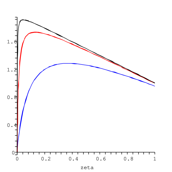
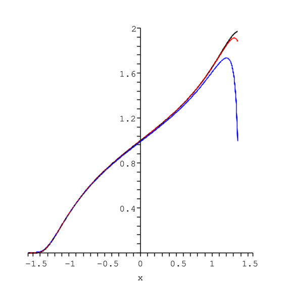
Figure 2: The inverse width $\sigma_{v}^{-2}$ of the off-diagonal matrix elements as a function of the degree of coherence of the distribution for $n=10^{1}$ (lower, blue), $n=10^{2}$ (middle, red), and $n=10^{3}$ (upper, black). Left panel, as a function of $\zeta=\delta/n$, one clearly sees the extreme sensitivity of $\sigma_{v}$ with respect to $\delta$ for small values. On the right panel, the same spread as function of $x=\arctan(\ln(\delta))$. This further shows that, for all values of $n\gg 1$, the critical regime is centered around $\delta=1$, i.e. the ‘grain’ of coherent states.

D.4 Sub-fluctuant mode and the power of the decaying mode

From the second equation in (C.2), we see that the sub-fluctuant mode behaves as

$$\langle\{\Pi_{\bf k},\,\Pi^{\dagger}_{\bf k}\}\rangle=\left(\frac{\delta}{2}+\frac{(1+\delta)^{2}}{8n}+O(n^{-2})\right)\,.$$ (148)

Therefore one looses the squeezed spread, i.e. $\langle\{\Pi_{\bf k},\,\Pi^{\dagger}_{\bf k}\}\rangle\geq 1/2$, when $\delta\geq 1$. In conclusion, one has

$${\rm{no\,\,\,subfluctuant\,\,\,variable}}\quad\Longleftrightarrow\quad\delta\geq 1\,.$$ (149)

It is interesting to notice that the value of the quantum coherence $\sigma_{v}$ and that of the squeezed spread are correlated. Indeed, their product obeys

$$\sigma_{v}^{2}\,\langle\{\Pi_{\bf k},\,\Pi^{\dagger}_{\bf k}\}\rangle=\frac{1+\delta}{4}\left(1+O(\frac{1}{n},\frac{\delta}{n})\right)\,,$$ (150)

for $0\leq\delta\ll n$. (This result is non-trivial for $\delta\leq 1/n$.) In Fig. 3, we have represented the plot of this product for the whole range of $\delta$. It is growing with $\delta$, the lower bound $1/4$ being reached for pure (squeezed) states. More importantly it stays almost constant for $\delta\leq 1$ before growing linearly with $\delta$ for $\delta\gg 1$.

The first regime corresponds to the loss of the quantum coherence whereas the second corresponds to the linear growth of the power of the subfluctuant mode (since $\sigma_{v}^{2}$ stays $\simeq 1$). At this point it is important to notice that this second regime also corresponds to a linear growth of the power of the decaying mode. Indeed, the powers of the subfluctuant mode and the decaying mode are related by

$$\langle\{d_{\bf k},\,d^{\dagger}_{{\bf k}}\}\rangle = \langle\{\Pi_{\bf k},\,\Pi^{\dagger}_{\bf k}\}\rangle+|c|(1-\cos 2\theta)$$ (151)

$$= \langle\{\Pi_{\bf k},\,\Pi^{\dagger}_{\bf k}\}\rangle+O(n^{-1/2})=\frac{\delta}{2}+O(n^{-1/2})\,,$$

where $\theta$ is defined in Eq. (31). In the second line, we have used the inflationary value of $\theta$ ($\propto n^{-3/4}$) and the fact that $\theta$ is unchanged when increasing $\delta$.

Similarly, the cross-correlation is

$$\langle\{d_{\bf k},\,g^{\dagger}_{{\bf k}}\}\rangle=-\sin(2\theta)|c|\,\propto n^{1/4}\left(1+\frac{1-\delta}{2n}+O(n^{-2})\right)\,.$$ (152)

One sees that the cross term is unaffected as long as $\delta\ll n$.

Figure 3: The product of the width $\sigma_{v}^{2}$ with the power of the subfluctuant mode, for $n=10^{1}$ (upper, blue), $n=10^{2}$ (middle, red), and $n=10^{3}$ (lower, black). For the horizontal axis, we used the non-linear scale $x=\arctan(\ln(\delta))$ of Fig 2. For the vertical axis, we used the non-linear scale $y=\arctan(\sigma_{v}^{2}\langle\{\Pi_{\bf k},\,\Pi_{-\bf k}\}\rangle)$. One clearly sees that for all $n\gg 1$, the product of Eq. (150) stays between $1/4$ and $1/2$ as long as $\delta\leq 1$. One also verifies that it is asymptotically $n$-independent for all values of $\delta\ll n$. Finally we recall that the power of the decaying mode coincides, to leading order, with $\langle\{\Pi_{\bf k},\,\Pi_{-\bf k}\}\rangle$, see Eq. (151).

D.5 $P$-representability of partially decohered density matrices

We now discuss the notion of $P$-representability of a density matrix Glauber63b . It is an intrinsic property of states which enlightens the distinct behaviours of quantum and classical distributions.

A one-mode density matrix is said to be $P$-representable if it can be written as a mixture of coherent states

$$\hat{\rho}_{P-\rm{repr}}=\int\!\!\frac{d^{2}v}{\pi}\,P(v)\,\mbox{$|v,\,{\bf k}\rangle$}\mbox{$\langle v,\,{\bf k}|$}\,,$$ (153)

where the weight function $P(v)$ is a tempered distribution Cahill65 ; Wodkiewiczlecture . Therefore, when considering $P$-representable Gaussian density matrices, the weight function $P(v)$ is simply a Gaussian function. The generalization of this definition to two-mode (Gaussian) distributions is straightforward:

$$\hat{\rho}_{P-\rm{repr}}=\int\!\!\frac{d^{2}v}{\pi}\frac{d^{2}w}{\pi}\,P(v,w)\,\mbox{$|v,\,{\bf k}\rangle$}\mbox{$\langle v,\,{\bf k}|$}\otimes\mbox{$|w,\,-{\bf k}\rangle$}\mbox{$\langle w,\,-{\bf k}|$}\,.$$ (154)

The $P$-representation of the distribution characterized by Eqs. (21) can easily be calculated. From (154), one calculates the expectation values ${\rm Tr}(\hat{n}_{k}\hat{\rho}_{P-\rm{repr}})=n$ and ${\rm Tr}(\hat{a}_{\bf k}\hat{a}_{-{\bf k}}\hat{\rho}_{P-\rm{repr}})=c$, and one gets

$$P(v,w)=\frac{1}{\Delta^{\prime}}\exp\left[-\frac{\mbox{$|v|$}^{2}}{n}-\frac{n}{\Delta^{\prime}}\mbox{$|w-(cv^{*}/n)|$}^{2}\right]\,,$$ (155)

where $\Delta^{\prime}=n^{2}-\mbox{$|c|$}^{2}$ must be positive. The function $P$ is well defined if, and only if, $n\geq\mbox{$|c|$}$, i.e. $\delta\geq n/(n+1)$. Hence, in the high occupation number limit,

$${\rm{P-representability}}\quad\Longleftrightarrow\quad\delta\geq 1\,.$$ (156)

This condition coincides with that for the non-existence of a sub-fluctuant variable, see Eq. (148), as well as that for the vanishing of the off-diagonal matrix elements, see Eq. (D.3). It also coincides with the condition obtained from the criterion of separability we shall discuss in the next subsection, see Eq. (159). This proves that all quantum properties are lost if, and only if, $\delta\geq 1$.

It is therefore of interest to further analyze this case and to determine how it is related to two-mode coherent states. Consider the limiting case $\Delta^{\prime}\to 0^{+}$, i.e. $\delta\to n/(n+1)$ from above. In this limit $P(v,w)$ of Eq. (155) becomes

$$P_{lim}(v,w)=\frac{1}{n}\exp\left[-\frac{\mbox{$|v|$}^{2}}{n}\right]\,\delta^{(2)}\left(w-\frac{c}{n}v^{*}\right)\,.$$ (157)

The presence of the two Dirac functions constraining the real and imaginary parts of $w$ clearly expresses the critical character of this distribution.

One can now notice that this distribution corresponds to the simplified distribution of Eq. (61). More precisely, the equality of the entropies, see Appendix D.7, suggest that (157) is the quantum counterpart of the classical effective classical distribution Eqs. (37-39) obtained by setting the decaying mode to zero. The (badly named) minimally decohered distribution (58) is in fact slightly more decohered as can be understood from the replacement of the Dirac’s $\delta^{(2)}\left(w-\frac{c}{n}v^{*}\right)$ by a Gaussian with a width equal to 1. This subtle difference is better appreciated when one realizes that the simplified distribution of Eq. (61) and that of (58), which are both diagonal in two-mode coherent states, belong to the same class of decohered matrices when considering the entropy.

D.6 Separability of two-mode homogeneous distributions and violations of Bell’s inequalities

The non-separability is another important criterion for distinguishing distributions which cannot be viewed as classical stochastic distributions. Its physical relevance comes from the fact that the non-separability is a necessary property to have expectation values violating Bell’s inequalitiesWerner89 . At the end of this subsection, we have included a brief discussion concerning the relationship between decoherence and the associated loss of the violation of Bell’s inequalities. For more details we refer to CP4 .

A word of caution is in order. Unlike the $P$-representability the non-separability rests on a division of the $4$ canonical variables into two subsets of $2$ canonical variables. To define the two subsets, we use creation and destruction operators carrying a momentum ${\bf k}$ or ${\bf-k}$. The criterion should therefore be called the $({\bf k},{\bf-k})$-separability. The justification of the choice of the two subsets is presented after having explained the concept of separability.

Following Werner Werner89 , a distribution of two-modes $\bf k$ and $-{\bf k}$ is said to be separable if, and only if, it can be written as a convex sum of products of distributions, i.e.

$$\hat{\rho}_{sep}=\sum_{l}p_{l}\,\hat{\rho}_{\bf k}^{(l)}\otimes\hat{\rho}_{-{\bf k}}^{(l)}\,,\qquad p_{l}\geq 0\,,\qquad\sum_{l}p_{l}=1\,.$$ (158)

Notice that the definition (158) is not the statement that a separable state is a product of its reduced density matrices (in which case one would obtain uncorrelated sub-systems: $p_{l}=0$ for all $l$ but one).

The key point is that all states of the form (158) can be obtained by the following classical protocol: when a random generator produces the number $l$ with probability $p_{l}$, two distant observers performing separate measurements on the subsystems $\bf k$ and $-{\bf k}$ respectively, prepare them into the states $\hat{\rho}_{\pm{\bf k}}^{(l)}$. Separable states are said classically correlated because, by construction, their statistical properties can be interpreted classically. In particular they cannot violate Bell’s inequalities. States which are not separable are called “entangled” (such as a two-mode squeezed vacuum states, or a singlet of $1/2$ spins) and can only be produced by letting the two parts of the system interact.

Although it may be very difficult to decipher the separability of a general two-mode state, there is a criterion for Gaussian states. We briefly outline the proof of this theorem, the complete proof can be found in Simon00 . First, one notices on (158) that the separability is a property that is not affected by local unitary transformations $U_{loc}=U_{{\bf k}}\otimes\tilde{U}_{-{\bf k}}$. These local transformations are of two types, rotations and squeezing which do not mix $\bf k$ and $\bf-k$. Therefore, if $\hat{\rho}$ is a separable state, then all states $\hat{\rho}\,^{\prime}=U_{loc}\,\hat{\rho}\,U_{loc}$ are also separable. Second, one notices that if $\hat{\rho}$ is a $P$-representable state (154), it is separable. The non trivial part of the proof consists then to show that all Gaussian separable states can be constructed by applying local unitary transformations on a $P$-representable state. In brief, the criterion for separability for two-mode Gaussian states is a Gaussian state $\hat{\rho}$ is separable if, and only if there is a local unitary transformation $U_{loc}$ which brings it to a $P$-representable state.

These local transformations are very constrained for homogeneous states because any local squeezing would break the homogeneity of the state (one would have either $\langle\hat{a}_{\bf k}^{2}\rangle\neq 0$ or $\langle\hat{a}_{\bf-k}^{2}\rangle\neq 0$, or both). Hence, $U_{loc}$ can only be a product of local rotations. These preserve the non-negativity of the Gaussian function $P(v,w)$. As a result, separability and $P$-representability are equivalent properties of homogeneous Gaussian states. Given (156), one concludes

$$({\bf k},-{\bf k})-{\rm{{separability\,\,\,of\,\,\,homogeneous\,\,\,states}}}\quad\Longleftrightarrow\quad\delta\geq 1\,.$$ (159)

Notice that the $({\bf k},{\bf-k})$-separability and the $(\phi_{1},\phi_{2})$-separability are two independent properties of the state. The former implies the above inequality on the decoherence level. As shown in Appendix C, the latter is simply a consequence of homogeneity of the distribution. The independence of these two concepts can be understood by noticing that the separability defines an equivalent class of density matrices through local transformations only. In fact, the transformation from the operators with a definite momentum ${\bf k}$ to ($\phi_{1}$, $\phi_{2}$) is a global, $4$ by $4$, transformation, see (120).

We should now explain the selection of the two subsets. The choice of $(\hat{a}_{\bf k},\,\hat{a}^{\dagger}_{\bf k})$ and $(\hat{a}_{\bf-k},\,\hat{a}^{\dagger}_{\bf-k})$, and not $(\hat{a}_{1},\,\hat{a}^{\dagger}_{1})$ and $(\hat{a}_{2},\,\hat{a}^{\dagger}_{2})$, is dictated by the nature of the interactions amongst modes. When keeping non-linear terms, the Lagrangian density is a sum of products of fields evaluated at the same point. This leads to terms of the form $\phi_{{\bf k}}\phi_{{\bf p}}\phi_{-{\bf k}-{\bf p}}$ which are governed by the Fourier transform of the field $\phi(\eta,{\bf x})$. These non-linear terms give rise to momentum exchanges which cannot be described by $\hat{a}_{1}$ or $\hat{a}_{2}$ separately. (It should be noticed that these hermitian operators obey unusual commutation relations with the momentum operator $\hat{\bf P}$: $[\hat{\bf P},\,\hat{a}_{1,\,2}]=\mp i{\bf k}\,\hat{a}_{2,\,1}$).

Notice that contrary to non-linear interactions, bilinear couplings do not permit to dismiss $\phi_{1},\,\phi_{2}$. Indeed, consider a bilinear interaction with a random field by adding a coupling term $\int\!\!d^{3}x\,\hat{\phi}(\eta,{\bf x})\,\Psi(\eta,{\bf x})$ where $\Psi(\eta,{\bf x})$ is a real stochastic field. Then the preferred basis are still the real and imaginary parts of $\phi(\eta,{\bf x})$, see KiefPolStar98a . To verify this it suffices to decompose the interaction term in Fourier transform, use the reality condition of the stochastic field $\Psi(\eta,{\bf x})$ to get $\int\!\!\widetilde{d^{3}k}\,\left[\hat{\phi}_{1}(\eta,{\bf k})\,\Psi_{1}(\eta,{\bf k})+\hat{\phi}_{2}(\eta,{\bf k})\,\Psi_{2}(\eta,{\bf k})\right]$, and then use the homogeneous and isotropic character of the moments of $\Psi(\eta,{\bf x})$. In this we recover the fact that homogeneity implies that all Gaussian density matrices are $(\phi_{1},\,\phi_{2})$-factorizable.

It is nevertheless possible to consider observables which cannot be written in terms of $\hat{a}_{1}$ or $\hat{a}_{2}$ separately without introducing explicitely non-linear interactions. To this end one should exploit the cosmic variance, namely the fact we do not observe the mean value, but rather some realization of the ensemble. (We refer to Chap. V of CP04 for the procedure to extract some realization from the distribution, to Chap. VI for the calculation of observables associated with a given realization, and to the references of this work for the relationship between the role played by the interaction Hamiltonian in non-linear theories and the role of the projector introduced to extract some configurations from the mean.) In particular, upon specifying that a localized classical field configuration possessing a definite velocity (e.g. a localized wave packet made with running waves) has been realized/detected, the conditional expectation value of $\hat{\phi}(\eta,{\bf x})$ describes a pair of wave packets moving away from each other and which are spatially well separated. These wave packets localized both in ${\bf x}$ and ${\bf k}$ space are built with $\hat{a}_{\bf k}$ and $\hat{a}_{-{\bf k}}$ separately. Hence they cannot be written in terms of $\hat{a}_{1}$ or $\hat{a}_{2}$ separately.

Loss of violations of Bell inequalities

In Wodkievicz , the authors point out that the projectors on a given field configuration can violate Bell’s inequalities when evaluated in two-mode squeezed states. In CP4 , we extend their analysis by replacing the pure states by the partially decohered distributions of Eq. (137). We plot in Fig. $4$ the combination $(n+1)\cal C$ of Eq. ($11$) of CP4 as a function of the square field amplitude for $n=100$ and for three different values of $\delta$. The points over the horizontal line $(n+1){\cal C}=2$ give combinations of operators violating Bell’s inequalities. We observe that for $\delta>0.1$, there is no more violations. However, the combination $\cal C$ does not provide the operator which maximizes the violation. Hence, there might still be operators which violate Bell’s inequalities for $0.1\leq\delta<1$.

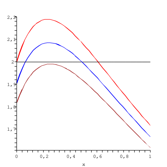
Figure 4: The loss of violation as decoherence increases. The function is normalized to its maximal classical value $=2$. The variable $x$ gives the square field amplitude. The occupation number is $n=100$, and the three values of $\delta$ are $0$ (red, upper), the pure state, $0.05$ (blue, middle), and $0.1$ (brown, lower), the border regime. It is also worth to point out that the function $(n+1){\cal C}(x)$ is independent of $n$ in the large $n$ limit as what is found in Figs. 3, 5, and 6.

D.7 Entropy of partially decohered distributions

     

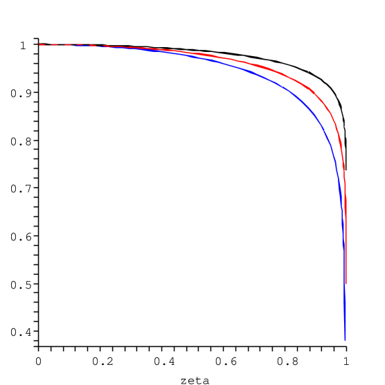
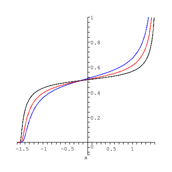
Figure 5: Entropy as a function degree of coherence for three values of $n$. The function is normalized to it maximal value. The occupation number is $n=10^{2}$ (lower, blue), $n=10^{3}$ (middle, red), and $n=10^{5}$ (upper, black). On the left panel, as a function of the ratio $\zeta=\mbox{$|c|$}/(n+1/2)$, one clearly see the sensitivity for $\zeta\to 1^{-}$. On the right panel, as a function of $x=\arctan(\ln(\delta))$, one verifies that the critical value $S_{max}/2$ corresponds to $\delta=1$ for all $n$.

To characterize the entropy of the general distribution (137), we write $\delta=An^{\gamma},\,A>0,\,1\geq\gamma\geq 0$. As we shall see, in the high occupation number limit, $\gamma$ is tightly constrained.

The thermal occupation number defined in Eq. (65) and the entropy respectively scale as

$$\bar{n}=\sqrt{A}n^{(1+\gamma)/2}+O(n^{-(1+\gamma)/2})\,,$$ (160)

and

$$S^{(\gamma,A)}_{{\bf k},\,-{\bf k}}=(1+\gamma)2r+\left(2+\ln A\right)+O(n^{-(1+\gamma)/2})\,.$$ (161)

We have used the squeezing parameter $n=\mbox{sh}^{2}(r)$. From this analysis we see that the uncertainty in the definition of the quantum distributions which gives rise to the entropy of the effective distribution of sine functions of (39) is very limited. (The entropy of that distribution is $S_{{\bf k},\,-{\bf k}}=2r$, see Eq. (67) and the discussion in the following paragraphs.) Indeed, the linear dependence of the entropy in $r$ implies that the distributions with entropy $=2r$ all have

$$\gamma\ll\frac{1}{\ln n}\,.$$ (162)

When refining the analysis by taking into account the term in $\ln A$, and requiring that $|S_{{\bf k},\,-{\bf k}}-2(r+1)|\leq B$, one gets $|\ln\delta|\simeq\delta-1\leq B$, independently of $n$. In the large $n$ limit, this fixes the value of the coherence term $c$ with a precision $B/n$, thereby tightly restricting the quantum density matrices which can be put in correspondence with Eq. (39).

Nevertheless, the criterium $S_{{\bf k},\,-{\bf k}}=2r+O(1)$ does not discriminate between the distribution of Eq. (58) ($\delta=2$) and that of Eq. (61) ($\delta=1$). Hence the distribution (58) should be conceived as minimal only as being a member of the equivalent class of minimally decohered matrices, i.e. those which have lost their quantum properties ($\delta>1$) and which possess an entropy equal to $2r$.

     

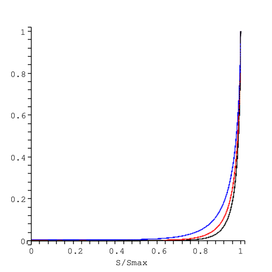
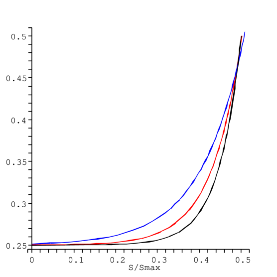
Figure 6: Parametric curves We plot the product $\sigma^{2}_{v}\langle\{\Pi_{\bf k},\,\Pi_{-{\bf k}}\}\rangle$ versus the entropy. The latter (horizontal axis) has been normalized to its maximum value $S_{max}$. The occupation number is $n=10^{2}$ (upper, blue), $n=10^{3}$ (middle, red), and $n=10^{5}$ (lower, black). On the left panel, $\delta$ goes from $0$ to $n$ and the product $\sigma^{2}_{v}\langle\{\Pi_{\bf k},\,\Pi_{-{\bf k}}\}\rangle$ has been normalized to its maximum value $n$. On the right panel, we show a zoom on the region $\delta\leq 1$, and the product is not normalized. One sees the two regimes. First as long as the entropy has not reached half its maximum value, the product stays nearly constant. On the contrary, for $S>S_{max}/2$, the product explodes and reaches $n$. One can also admire the fact that the curves meet near $(1/2,1/2)$ irrespectively of the value of $n$. Moreover in the limit $n\to\infty$ the curve becomes an Heavyside function, thereby cleary separating the two regimes: the first one where quantum properties are progressively lost, and the second one where the power of the decaying mode linearly grows with $\delta$.

D.8 Partial randomization of the phase

To complete the analysis we now assume that the phase of the squeezed vacuum state is randomly scattered. The density matrix $\hat{\rho}_{in}$ is then replaced by the statistical mixture

$$\hat{\rho}(r,\varphi_{0})=\int_{0}^{2\pi}\!\!d\varphi\,f(\varphi;\,\varphi_{0},\,\sigma)\hat{\rho}_{in}(r,\,\varphi)\,,$$ (163)

where each pure state $\hat{\rho}_{in}(r,\,\varphi)$ is parameterized by the squeezing parameters $r$ and $\varphi$, and $f(\varphi;\,\varphi_{0},\,\sigma)$ is the PDF of $\varphi$ centered at $\varphi_{0}$ with a spread $\sigma$. We assume that the mean phase shift vanishes. Therefore the mean value of $\varphi$ is the phase of the original distribution (18), namely $\varphi_{0}=\pi+2k\eta_{r}$.

Since all the states in the ensemble (163) have the same value of $r$, the expectation value of the occupation number is still $\langle\hat{a}_{\pm{\bf k}}^{\dagger}\hat{a}_{\pm{\bf k}}\rangle=\mbox{sh}^{2}r=n$. However the effective coherence term is reduced since it is affected by averaging over the phase :

$$\langle\!\langle\,c\,\rangle\!\rangle_{\varphi}={\rm Tr}\left(\hat{a}_{{\bf k}}\hat{a}_{-{\bf k}}\hat{\rho}(r,\varphi_{0})\right)=\sqrt{n(n+1)}\int_{0}^{2\pi}\!\!d\varphi\,f(\varphi)e^{i\varphi}\,.$$ (164)

Let us assume that the function $f(\varphi)$ is sharply peaked. Then we can extend the bounds of integration to infinity. Let us choose for instance a Gaussian PDF, $f(\varphi)=(2\pi\sigma^{2})^{-1/2}\exp\left(-(\varphi-\varphi_{0})^{2}/2\sigma^{2}\right)$. One gets

$$\langle\!\langle\,c\,\rangle\!\rangle_{\varphi}=\sqrt{n(n+1)}e^{i\varphi_{0}}e^{-\sigma^{2}/2}\,.$$ (165)

Hence, we have that $\mbox{$|\langle\!\langle\,c\,\rangle\!\rangle_{\varphi}|$}=\mbox{$|c_{sq}(r)|$}e^{-\sigma^{2}/2}<\mbox{$|c_{sq}(r)|$}$, i.e. the norm of the effective coherence term is smaller, as expected. A value $\delta_{cr}=1$ corresponds to an extremely narrow distribution: $\sigma_{cr}^{2}=1/(n+1)=4(k\eta_{r})^{4}\sim 10^{-100}$. It should be noticed that these changes affecting the coherence are much smaller than those obtained when considering the trans-Planckian problem, see NP ; NPC ; MB , which concerned modifications of the power $n(k)$.

References

- (1) V. Mukhanov, C. Chibisov, JETP Lett. , No. 10, 532 (1981), astro-ph/0303077.
- (2) A.A. Starobinsky, JETP Lett. , 682 (1979), and Phys.Lett. B , 175 (1982).
- (3) S. Hawking, Phys.Lett. B , 295 (1982).
- (4) A. Guth and S.Y. Pi, Phys.Rev.Lett. , 1110 (1982).
- (5) J.M. Bardeen, P.J. Steinhardt, M.S. Turner, Phys.Rev. D, 679 (1983).
- (6) L.P. Grishchuk and Yu.V. Sidorov, Phys. Rev. D, 3413 (1990).
- (7) A.R. Liddle, D.H. Lyth, Phys.Rept. 231, 1 (1993).
- (8) A. Albrecht, Presented at NATO Advanced Study Institute: Structure Formation in the Universe, Cambridge, England, 26 Jul - 6 Aug 1999, astro-ph/0007247.
- (9) R.F. Werner, Phys.Rev.A , 4277 (1989).
- (10) K.E. Cahill and R.J. Glauber, Phys. Rev.177, 1882 (1969).
- (11) W.H. Zurek, in The Physics of Time Asymmetry, edited by J.J. Halliwell, J. Perez-Mercader, and W.H. Zurek, (Cambridge University Press, Cambridge, UK, 1993): Theor. Phys.
- (12) W.H. Zurek, S. Habib, J. P. Paz, Phys.Rev.Lett. , 1187 (1993).
- (13) J. Maldacena, JHEP , 013 (2003).
- (14) K. Gottfried, Chap. IV in Quantum Mechanics, Vol. I, Benjamin, New York, 1966.
- (15) U. Seljak, M. Zaldarriaga, Astrophys.J. 469, 437 (1996).
- (16) R. Brandenberger, V. Mukhanov, and T. Prokopec, Phys.Rev.Lett. , 3606 (1992); and Phys.Rev. D, 2443(1993).
- (17) T. Prokopec, Class. Quant. Grav. 10 229 (1993); and A. Albrecht, P. Ferreira, M. Joyce, and T. Prokopec, Phys.Rev. D , 4807 (1994).
- (18) A.L. Matacz, Phys.Rev. D, 788 (1994).
- (19) M.Gasperini and M.Giovannini, Phys. Lett. B, 334 (1993); and Class. Quant. Grav. , L133 (1993); and ’String Theory in Curved space Times’, (World Scientific, Singapore, 1998), p.249.
- (20) D. Polarski and A.A. Starobinsky, Class. Quant. Grav. , 377 (1996).
- (21) C. Kiefer, D. Polarski, and A.A. Starobinsky, Int.J.Mod.Phys. D, 455 (1998); and C. Kiefer and D. Polarski, Annalen Phys. , 137 (1998).
- (22) C. Kiefer, D. Polarski, and A.A. Starobinsky, Phys.Rev. D, 043518 (2000).
- (23) D. Campo and R. Parentani, Inflationary spectra, decoherence, and two-mode coherent states, astro-ph/.
- (24) V. Mukhanov, H. Feldman, and R. Brandenberger, Phys.Rep. , 203 (1992).
- (25) V. Mukhanov, astro-ph/0303072.
- (26) N.D. Birrel and P.C.W. Davis, in Quantum Fields in Curved Space (Cambridge University Press, Cambridge, UK, 1984).
- (27) J.C. Niemeyer, R. Parentani, and D. Campo, Phys.Rev. D, 0083510 (2002).
- (28) R. Parentani, C.R. Physique , 935 (2003).
- (29) R. Brout, S. Massar, R. Parentani, and Ph. Spindel, Phys.Rept. , 329 (1995).
- (30) H.V. Peiris & al., Astrophys.J.Suppl.148 213 (2003).
- (31) B. Allen, E. E. Flanagan, and M. A. Papa, Phys.Rev. D, 024024 (2000).
- (32) N. Bartolo, E. Komatsu, S. Matarrese, and A. Riotto, Phys.Rept. , 103 (2004).
- (33) D. Campo and R. Parentani, Phys.Rev. D, 105020 (2004).
- (34) H. Jeong, J. Lee, and M. S. Kim, Phys.Rev. A, 052101 (2000).
- (35) W.H. Zurek, Phys.Rev. D, 1516 (1981).
- (36) W.H. Zurek, Phys.Rev. D, 1862 (1982).
- (37) E. Joss and H. Zeh, Z. Phys. B,223 (1985).
- (38) A. Serafini, F. Illuminati, and S. De Siena, J.Phys. B,L21 (2004).
- (39) J. Martin and R. Brandenberger, Phys. Rev. D, 123501 (2001), ibid , 063513 (2003).
- (40) J.C. Niemeyer and R. Parentani, Phys.Rev. D, 101301(R) (2001).
- (41) M. Morikawa, Phys.Rev. D, 2929 (1990).
- (42) K. Banaszek and K. Wódkiewicz, Acta Phys.Slov. , 491 (1999).
- (43) D. Campo and R. Parentani, Inflationary spectra and violations of Bell’s inequalities, astro-ph/0505376; Quantum correlations in inflationary spectra and violation of Bell inequalities, Proceedings of the conference ”100 years in relativity”, Sao Paulo, August 22-24, to appear in a special issue of the Brazilian Journal of Physics (BJP), astro-ph/0510445,
- (44) E. Calzetta and B.L. Hu, Phys.Rev. D, 6770 (1995).
- (45) R.J. Glauber, Phys.Rev. , 2529 (1963).
- (46) R.J. Glauber, Phys.Rev. , 2766 (1963).
- (47) W.M. Zhang, D.H. Feng, and R. Gilmore, Rev.Mod.Phys. , 867 (1990).
- (48) B. Schumaker and C. Caves, Phys. Rev. , 3068; 3093 (1985).
- (49) R. Simon, Phys.Rev.Lett. , 2726 (2000); L-M. Duan, G. Giedke, J.I. Cirac, and P. Zoller, Phys.Rev.Lett. , 2722 (2000); B-G. Englert, and K. Wódkiewicz, Phys.Rev.A , 054303 (2002).
- (50) B-G. Englert, and K. Wódkiewicz, International Journal of Quantum Information 11, No. 2, 153 (2003).
- (51) H.M. Nussenzveig, Introduction to Quantum Optics, Gordon and Breach Science Publishers, New York, N.Y. (1973).
- (52) K.E. Cahill, Phys.Rev. , 1566 (1965).