Inflationary spectra and violations of Bell inequalities

Abstract

In spite of the macroscopic character of the primordial fluctuations, the standard inflationary distribution (that obtained using linear mode equations) exhibits inherently quantum properties, that is, properties which cannot be mimicked by any stochastic distribution. This is demonstrated by a Gedanken experiment for which certain Bell inequalities are violated. These violations are in principle measurable because, unlike for Hawking radiation from black holes, in inflationary cosmology we can have access to both members of correlated pairs of modes delivered in the same state. We then compute the effect of decoherence and show that the violations persist provided the decoherence level (and thus the entropy) lies below a certain non-vanishing threshold. Moreover, there exists a higher threshold above which no violation of any Bell inequality can occur. In this regime, the distributions are “separable” and can be interpreted as stochastic ensembles of fluctuations. Unfortunately, the precision which is required to have access to the quantum properties is so high that, in practice, an observational verification seems excluded.

The inflationary paradigm inflation0 successfully accounts for the properties of primordial spectra revealed by the combined analysis of CMBR temperature anisotropy and Large Scale Structure spectra WMAP . In particular, it predicts that the distribution of primordial fluctuations is homogeneous, isotropic and Gaussian, and that the power spectrum is nearly scale invariant (simply because the Hubble radius was slowly varying during inflation).

Surprisingly, inflation implies that density fluctuations arise from the amplification of vacuum fluctuations inflation ; because of backreaction effects, the vacuum is indeed the only possible initial state RenaudCMB . In addition of being amplified, the modes of opposite wave-vectors $\bf k$ and $-\bf k$ end up highly correlated. More precisely, using linear mode equations, the vacuum evolves into a product of two-mode squeezed states squeezing ; squeezing2 ; CaveSchumaker ; AllenFlanagan . The highly squeezed character of the distribution implies the vanishing of the variance in one direction in phase space. This direction is that of the decaying mode squeezing2 . The observational consequence of this squeezing are the acoustic peaks in the temperature anisotropy spectrum Albrecht ; Staroentropy .

In spite of the macroscopic character of the mode amplitudes, we shall show that the inflationary distribution is still entangled in a quantum mechanical sense. To prove this, we shall provide observables able to distinguish quantum correlations from stochastic correlations. At this point, it is important to notice that, unlike for Hawking radiation from black holes, we have in principle access to the purity of the state since, both members of two-mode sectors in the same state can be simultaneously observed on the last scattering surface CP2 .

Another important element should now be discussed: the linear mode equation is only approximate. Indeed, even in the simplest inflationary models there exists gravitational interactions which couple sectors with different $\bf k$’s, and induce non-Gaussianities Maldacena03 . However, as in the $BCS$ description of super-conductivity BCS , the weakness of the interactions allows to approximate the distribution by a product of Gaussian two-mode distributions Staroentropy ; CPfat . The non-linearities will then affect the power spectrum as if some decoherence effectively occurred. In this sense, inflationary distributions belong to the class of Gaussian homogeneous distributions obtained by slightly decohering the standard distribution derived with linear mode equations. Notice also that in general, we have an experimental access to the state of a system only through a truncated hierarchy of it’s Green functions, the Gaussian ansatz being the lowest order (Hartree) approximation.

In the absence of a clear evaluation of the importance of non-linearities , it is of value to phenomenologically analyze the above class. It is characterized by three $k$-dependent parameters. The first governs the power, see $n_{k}$ in (2). The second gives the orientation of the squeezed direction in phase space, whereas the third controls the strength of the correlations between modes with opposite momenta. The latter is strongly affected by decoherence effects, and shall be used to parameterize the decoherence level. It has been understood Albrecht ; Staroentropy that this level cannot be too high so as to preserve the well defined character of the acoustic peaks. However what is lacking in the literature concerning the quantum-to-classical transition is an operational identification of the subset of distributions exhibiting quantum correlations.

To fill the gap, we propose a Gedanken experiment which shows that certain Bell inequalities are violated when using the standard distribution. We then show that the violation persists provided that the decoherence level lies below a certain threshold. Finally we point that there exists a higher threshold above which no violation of any Bell inequality can occur. The corresponding distributions are separable (see below for the definition) and can be interpreted as stochastic ensembles.

In inflationary models based on one inflaton field, the linear metric (scalar and tensor) perturbations around the homogeneous background are governed by massless minimally coupled scalar fields obeying canonical commutation relations MukhaPhysRep . The scalar metric perturbations are driven by the inflaton fluctuations and correspond to perturbations along the background trajectory, called adiabatic perturbations Wands . At the end of inflation, the homogeneous inflaton condensate decays and heats up matter fields. After inflation, during the radiation dominated era, the adiabatic perturbations correspond to density perturbations of the matter fields (radiation, dark matter, …) which all start to oscillate in phase. The fluctuations orthogonal to these, called iso-curvature, are not excited on cosmological scales in one inflaton field models. Therefore, in the linear approximation, the phase and amplitude of the ${\bf k}$-th Fourier mode of each matter density fluctuation is related, via a time dependent transfer matrix, to the value of $\phi_{\bf k}$ and its time derivative evaluated at the end of inflation ($\phi$ being the canonical field governing scalar metric fluctuations during inflation). This implies that the properties of the correlations of the density fluctuations are the same as those of $\phi_{\bf k}$.

We now briefly outline how one obtains highly squeezed two-mode states squeezing ; squeezing2 . During inflation, in the linearized treatment, each $\phi_{\bf k}$ evolves under its own Hamiltonian

$$H_{\bf k}=\frac{1}{2}\,\left[|\partial_{\eta}\phi_{\bf k}|^{2}+\left(k^{2}-\frac{\partial_{\eta}^{2}a}{a}\right)\,|\phi_{\bf k}|^{2}\right]\,,$$ (1)

where $\eta$ is the conformal time $d\eta=dt/a$ and $a$ is the scale factor. To follow the mode evolution after the reheating time $\eta_{r}$, we continuously extend the inflationary law to a radiation dominated phase wherein $a\propto\eta$. In quantum settings, the initial state of the relevant modes (i.e. today observable in the CMBR) is fixed by the kinematics of inflation RenaudCMB : these were in their ground state about $70$ e-folds before the end of inflation (the minimal duration of inflation to include today’s Hubble scale inside a causal patch). From horizon crossing $k/a=H$ till the reheating time, $(k^{2}-\partial_{\eta}^{2}a/a)$ in (1) is negative. As a result, at the end of inflation, the initial vacuum has evolved into a tensor product of highly squeezed two-mode states.

The resulting distribution belongs to the class of Gaussian homogeneous distributions, see CPfat for more details. These are characterized by their two-point functions, best expressed as

$$\langle\hat{a}_{\bf k}^{\dagger}\,\hat{a}_{\bf k^{\prime}}\rangle=n_{k}\,\delta^{3}({\bf k}-{\bf k}^{\prime})\,,\quad\langle\hat{a}_{\bf k}\,\hat{a}_{\bf k^{\prime}}\rangle=c_{k}\,\delta^{3}({\bf k}+{\bf k}^{\prime})\,.$$ (2)

The destruction operator $\hat{a}_{\bf k}$ is defined by $\hat{a}_{\bf k}\,e^{-ik\eta_{r}}=\sqrt{k/2}(\hat{\phi}_{\bf k}+i\partial_{\eta}\hat{\phi}_{\bf k}/k)$ where $\hat{\phi}_{\bf k}$ is evaluated at $\eta_{r}$. The mean occupation number governs the power spectrum, as shall be explained after Eq. (Inflationary spectra and violations of Bell inequalities). To meet the observed r.m.s. amplitude of the order of $10^{-5}$, one needs $n_{k}\sim 10^{100}$, i.e. highly excited states. The phase $\arg(c_{k})$ gives the orientation of the squeezed direction in phase space at $\eta_{r}$. In inflation, using the above phase conventions, one gets $\arg(c_{k})=\pi+O(n_{k}^{-3/4})$. Finally, the norm of ${c_{k}}$ governs the strength of the correlations between partner modes ${\bf k},{-\bf k}$, i.e., the level of the coherence of the distribution. To parameterize the (de)coherence level, we shall work at fixed $n$ and $\arg(c)$ (in the sequel we drop the $k$ indexes), and write the norm $|c|$ as

$$\mbox{$|c|$}^{2}=(n+1)(n-\delta)\,.$$ (3)

The standard distribution obtained in the linear treatment is maximally coherent and corresponds to $\delta=0$. The least coherent distribution, a product of two thermal density matrices, corresponds to $\delta=n$.

The physical meaning of $\delta$ is revealed by decomposing the adiabatic modes in terms of the amplitudes ($g,d$) of the growing and decaying solutions. Taking into account the time dependence of the corresponding transfer matrix, any matter density fluctuation can be used. For simplicity, we shall use the massless field $\phi$ extended in the radiation dominated era. In this case, the transfer matrix of $\hat{a}_{\bf k}$ is simply $e^{-ik\eta}$. Decomposing

$$\hat{\phi}_{\bf k}(\eta)=\hat{g}_{\bf k}\frac{\sin(k\eta)}{\sqrt{k}}+\hat{d}_{\bf k}\frac{\cos(k\eta)}{\sqrt{k}}\,,$$ (4)

Eqs. (2) give

$$\langle\hat{g}_{\bf k}\hat{g}_{\bf k}^{\dagger}\rangle = n+\frac{1}{2}-Re(c)=2n\,\left(1+O(\frac{\delta}{n})\right)\,,$$

$$\langle\hat{d}_{\bf k}\hat{d}_{\bf k}^{\dagger}\rangle = n+\frac{1}{2}+Re(c)=\frac{\delta}{2}+O(n^{-1/2})\,.$$ (5)

The last expression in each line is valid when the decoherence is weak, i.e. $\delta\ll n$. In this regime, the power spectrum $P_{k}=k^{3}\langle\hat{\phi}_{\bf k}(\eta)\hat{\phi}_{-{\bf k}}(\eta)\rangle\simeq k^{2}n_{k}\sin^{2}(k\eta)$ is dominated by the growing mode. At fixed $\eta$, it therefore displays peaks and zeros as $k$ varies. From the last equation (Inflationary spectra and violations of Bell inequalities), one sees that the decoherence level $\delta$ fixes the power of the decaying mode. (The same conclusions would have been reached had we considered dark matter or temperature perturbations.)

Even though Eqs. (2) univocally determine the corresponding (Gaussian) distribution, they are unable to sort out the distributions possessing quantum properties from those which have lost them, or in other words, to determine the ranges of $\delta$ characterizing these two classes. To operationally do so, it is necessary to introduce operators which are not polynomial in $\hat{g}_{\bf k}$ and $\hat{d}_{\bf k}$ .

In what follows, we shall use operators based on coherent states. These obey $\hat{a}_{\bf k}\mbox{$|v,{\bf k}\rangle$}=v\mbox{$|v,{\bf k}\rangle$}$ and $\hat{a}_{\bf-k}\mbox{$|w,{\bf-k}\rangle$}=w\mbox{$|w,{\bf-k}\rangle$}$. They are minimal uncertainty states and each of them can be considered as the quantum counterpart of a point in phase space, here a classical fluctuation with definite phase and amplitude. This correspondence is excellent in the regime $n\gg 1$. Moreover, they play a key role when considering decoherence: when modes are weakly coupled to an environment, the reduced density matrix becomes diagonal in the basis of coherent states Zu , or other minimal uncertainty states E .

Coherent states are particularly useful in our context because they will allow us to sort out entangled quantum distributions from stochastic ones. The reason is that coherent states can probe the detailed properties of the distribution. In particular, the probability to find a particular classical fluctuation is given by the expectation value of the projector on the corresponding (two-mode) coherent state, namely

$$\Pi(v,w)=\mbox{$|v,{\bf k}\rangle$}\mbox{$\langle v,{\bf k}|$}\otimes\mbox{$|w,{\bf-k}\rangle$}\mbox{$\langle w,-{\bf k}|$}\,.$$ (6)

The probability is

$$Q(v,w;\delta) = {\rm Tr}[\rho_{2}(\delta)\,\Pi(v,w)]\,,$$ (7)

$$= \frac{1}{n+1}\exp\left[-\frac{\mbox{$|v|$}^{2}}{(n+1)}\right]\times$$

$$\quad\frac{1}{1+\delta}\exp\left[-\frac{\mbox{$|w-\bar{w}(v)|$}^{2}}{1+\delta}\right]\,,\quad$$

where $\rho_{2}(\delta)$ is the matrix density of the two-mode system. We have written $Q(v,w;\delta)$ in an asymmetric form to make explicit the power of the growing mode ($=n+1$), and the much smaller width ($={1+\delta}$) governing the dispersion of the values of $w$ around $\bar{w}(v)=v^{*}c/(n+1)$, the conditional amplitude of the partner mode, given $v$. Had we used a projector on a one-mode coherent state, we would have gotten only the first Gaussian. In fact, as we shall see, to have access to the (residual) quantum properties of the distribution, one must use the two-mode projectors (6). As explained in CP2 , these projectors also allow to compute conditional values which cannot be expressed in terms of mean values. For instance, ${\rm Tr}[\Pi\rho\Pi\,\hat{\phi}(\eta,{\bf x})]$ gives the space-time pattern of fluctuations when the set of configurations specified by the projector $\Pi$ is realized.

Given the macroscopic character of mode amplitudes in inflationary cosmology, it is remarkable that the projectors (6) can violate Bell inequalities. To understand the origin of this possibility, it is necessary to define the class of separable states Werner . A two-mode state is said separable if it can be written as a positive sum of products of one-mode density matrices Separable Gaussian states can all be written in terms of the projectors (6) as CPfat

$$\rho_{2}^{\rm sep.}(\delta)=\int\!\!\frac{d^{2}v}{\pi}\frac{d^{2}w}{\pi}\,P(v,w;\delta)\,\Pi(v,w)\,.$$ (8)

The function $P$ is given by

$$P(v,w;\delta) = \frac{1}{\Delta^{\prime}}\exp\left[-\frac{\mbox{$|v|$}^{2}}{n}\right]\times\exp\left[-\frac{\mbox{$|w-\tilde{w}|$}^{2}}{\Delta^{\prime}/n}\right]\,,\quad$$ (9)

with $\tilde{w}=cv^{*}/n$ and $\Delta^{\prime}=n^{2}-\mbox{$|c|$}^{2}\geq 0$. The latter implies $\mbox{$|c|$}\leq n$, or $\delta\geq n/(n+1)\simeq 1$ for $n\gg 1$. (The limiting case $\mbox{$|c|$}=n$, $\delta=n/(n+1)$ is interesting: the second exponential becomes a double Dirac delta which enforces $w=cv^{*}/n=-v^{*}$ in phase and amplitude. In other words, for each two-mode sector, there is only one fluctuating quantity, since the second mode is completely fixed by its partner. In inflationary cosmology, the corresponding density matrix can be viewed as the quantum analogue of the usual stochastic distribution of growing modes. Indeed, the entropy of this quantum distribution is $\ln(n)$ per two-mode, and this is the entropy of the stochastic distribution for each growing mode CPfat . This quantum-to-classical correspondence is corroborated by the fact that off-diagonal matrix elements of $\rho(\delta)$ in the coherent state basis vanish precisely when $\delta>1$.

The physical meaning of separable states comes from the fact that all states of the form (8) can be obtained by the following classical protocol Werner : when a random generator produces the four real numbers encoded in $(v,w)$ with probability $P$, two space-like separated observers performing separate measurements on the subsystems $\bf k$ and $-{\bf k}$ respectively, prepare them into the two-mode coherent state $|v\rangle$$|w\rangle$. Non-separable states can only be produced by letting the two parts of the system interact. Only these are quantum mechanically entangled.

By construction, the statistical properties of separable states can be interpreted classically. In particular, they cannot violate Bell inequalities Werner . In what follows we shall study the “Clauser-Horne” inequality CH ; Wodkievicz98 because it is based on $Q$ of (7). It reads

$${\cal C}(v,w;\delta) = [Q(0,0;\delta)+Q(v,0;\delta)$$

$$+\,Q(0,w;\delta)-Q(v,w;\delta)]\times\left(\frac{n+1}{2}\right)\leq 1\,.$$

We can now search for distributions, i.e. values of $\delta$, and for configurations $v$ and $w$ which maximize ${\cal C}$. The maximization with respect to $w$ gives $\arg(c^{*}vw)=\pi$ and $\mbox{$|w|$}=\mbox{$|v|$}$. We fix the arbitrary phase of $v$ by $2\arg(v)=\arg(c)$, so that ${\cal C}$ is maximum along the ’line’ $w=-v$. In Fig. 1 we have plotted ${\cal C}(v,-v,\delta)$ for three values of $\delta$.

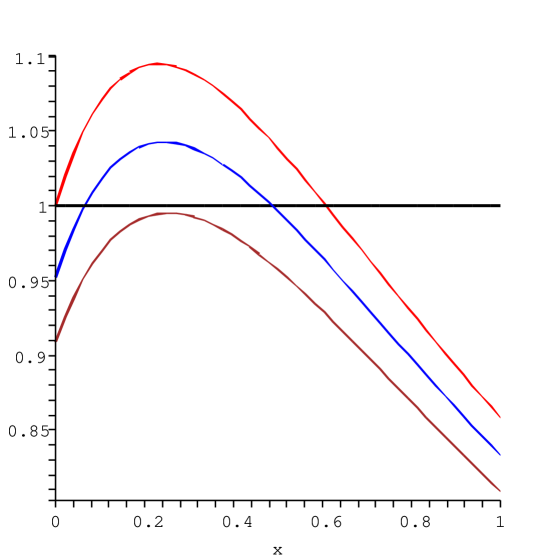
Figure 1: The loss of violation as decoherence increases. We have represented ${\cal C}(v,-v,\delta)$ as a function of $x=\mbox{$|v|$}^{2}$ for $n=100$ and for three values of $\delta$: $0$ (upper), $0.05$ (middle), and $0.1$ (lower). The horizontal line (${\cal C}=1$) is the maximal value allowed by classically correlated states.

The maximum with respect to the norm of $v$ is reached for

$$\frac{\mbox{$|v_{M}(\delta)|$}^{2}}{1+\delta} = \frac{\ln\left[1+\sqrt{\frac{n-\delta}{n+1}}\right]}{1+2\sqrt{\frac{n-\delta}{n+1}}}=\frac{\ln 2}{3}\left[1+O(\delta/n)\right]\,.\quad$$ (11)

The maximal value is

$${\cal C}_{M}(\delta) = \frac{1}{2(1+\delta)}\times\left[1+\frac{3}{2^{4/3}}+O\left(\frac{1+\delta}{n}\right)\right]\,.\quad\quad$$ (12)

The inequality (Inflationary spectra and violations of Bell inequalities) is thus violated for

$$\delta<\frac{-1+3/2^{4/3}}{2}\simeq 0.095\,,$$ (13)

irrespectively of the value of $n$ when $n\gg 1$.

From the last two equations we learn that Bell inequality (Inflationary spectra and violations of Bell inequalities) is violated by the standard inflationary distribution ($\delta=0$). Notice that this violation is maximal, as one might have expected, since the two-mode correlations are the strongest in this state. More importantly, if $\delta$ obeys (13), the violation persists in the regime of highly amplified modes obtained in inflationary cosmology.

In conclusion, the principle results of this Rapid Communication are the following. First, in spite of the macroscopic character of adiabatic fluctuations, the standard inflationary distribution possesses quantum features which cannot be mimicked by any stochastic distribution. Second, these features are operationally revealed by a well defined procedure based on the violation of the Bell inequality (Inflationary spectra and violations of Bell inequalities). Third, the projectors used in this inequality have a clear meaning in cosmology: they give the probability that a particular semi-classical fluctuation be realized. Fourth, the mere existence of decoherence effects is not sufficient to eliminate the quantum properties. To do so, decoherence should be strong enough so as to induce $\delta\geq 1$, that is, so that the distribution becomes separable.

The threshold value $\delta=1$ therefore plays a double role. First, as previously noticed, the distribution with $\delta=1$ possesses an entropy ($=\ln n$ per two-mode) which is equal to that of the classical distribution of growing modes. Second, separability is the condition for distinguishing quantum from classical distributions, see e.g. Halliwell where it was used to define the time of decoherence. To our knowledge, besides the present work, this criterion of the study of the quantum-to-classical transition has not been used in inflationary cosmology.

Let us now briefly address two additional questions. Firstly, to what extend the violation of the inequality (Inflationary spectra and violations of Bell inequalities) is verifiable ? We start by pointing out that there is no physical principle which prevents evaluating the four terms in Eq. (Inflationary spectra and violations of Bell inequalities). Because of isotropy, in a given comoving volume (e.g. a sphere of radius $R$), we have, for a given wave vector norm $k=|{\bf k}|$, about $(kR)^{2}$ adiabatic modes all characterized by the same two-mode density matrix. This is true before and after the reheating, and also irrespectively of the decoherence level. Finally this is still true when considering the projection of the adiabatic modes on the last scattering surface. Indeed, for sufficiently high angular momentum, there exist an ensemble of well aligned two-modes with both members living on the last scattering surface CP2 . One can thus accumulate statistics to measure the four observables of Eq. (Inflationary spectra and violations of Bell inequalities). Unfortunately, an observational verification of the inequality Eq. (Inflationary spectra and violations of Bell inequalities) seems excluded. Indeed the cosmic variance, which is of the order of the mean amplitude (hence proportional to $n\sim 10^{100}$), is much larger than the required precision, which is given by the spread of the coherent states ($=1$)

The second question concerns the value of $\delta$ in realistic inflationary models. This interesting question deserves further study, see the Added Note. Let us here simply compare the critical value $\delta=1$ separating quantum from stochastic distributions to the expected level of non-Gaussianities. At the end of inflation, the two-point function of the gravitational potential $\Psi$ is conventionally Komatsu parameterized by the coefficient $f_{N\!L}$ entering the field redefinition $\Psi=\left[\phi+f_{N\!L}\,\phi^{2}/(aM)\right]/(\sqrt{\epsilon}Ma)$ where $\phi$ is our Gaussian field during inflation, $M$ is Planck mass, and $\epsilon$ the slow roll parameter. It has been observationally limited to $-58<f_{N\!L}<134$ WMAP , while theoretical calculations give $f_{N\!L}=O(10^{-2})$ for the inflationary phase. On one hand, the variation of the power spectrum of $\Psi$ is therefore $\Delta P/P\simeq f_{N\!L}^{2}P$ where $P$ is the power spectrum in the linear approximation ($\simeq 10^{-10}$). On the other hand, using (Inflationary spectra and violations of Bell inequalities), one gets $\Delta P/P=\delta/n$. Therefore $f_{N\!L}=10^{-2}$ corresponds t $\delta\simeq nPf_{N\!L}^{2}\simeq 10^{86}$. This indicates that the minimal source of decoherence, the non-linear interactions during inflation, should be strong enough to give rise to separable distributions.

Acknowledgements: We would like to thank Ulf Leonhardt and Serge Massar for interesting discussions and suggestions.

References

- (1) V. Mukhanov, Physical Foundations of Cosmology (Cambridge University Press, New York, 2005).
- (2) C. L. Bennett et al., Astrophys. J. Suppl. 148 (2003) 1.
- (3) V. Mukhanov, C. Chibisov, JETP Lett. , No. 10, 532 (1981); A.A. Starobinsky, JETP Lett. , 682 (1979), and Phys. Lett. B (1982) 175; S. Hawking, Phys. Lett. B (1982) 295; A. Guth and S.Y. Pi, Phys. Rev. Lett. (1982) 1110; J.M. Bardeen, P.J. Steinhardt, M.S. Turner, Phys. Rev. D (1983) 679.
- (4) R. Parentani, C. R. Physique , 935 (2003).
- (5) L. Parker, Phys. Rev. , 1057 (1969); L.P. Grishchuk and Yu.V. Sidorov, Phys. Rev. D , 3413 (1990).
- (6) C.M. Caves and B.L. Schumaker, Phys. Rev. A , 3068 (1985); ibid. 3093.
- (7) A. Albrecht, P. Ferreira, M. Joyce, and T. Prokopec, Phys. Rev. D , 4807 (1994); D. Polarski and A. A. Starobinsky, Class. Quant. Grav. , 377 (1996).
- (8) B. Allen, E.E. Flanagan, and M.A. Papa Phys. Rev. D 61, 024024 (2000).
- (9) A. Albrecht, D. Coulson, P. Ferreira, and J. Magueijo, Phys. Rev. Lett. , 1413 (1996).
- (10) C. Kiefer, D. Polarski, and A.A. Starobinsky, Phys. Rev. D , 043518 (2000).
- (11) D. Campo and R. Parentani, Phys. Rev. D , 105020 (2004).
- (12) J. Maldacena, JHEP , 013 (2003).
- (13) J. Bardeen, L.N. Cooper, and J.R. Schrieffer Phys. Rev. , 1175 (1957).
- (14) D. Campo and R. Parentani, Phys. Rev. D , 045015 (2005).
- (15) P. Martineau, astro-ph/0601134; C.P. Burgess, R. Holman and D. Hoover, astro-ph/0601646.
- (16) V. Mukhanov, H. Feldman, and R. Brandenberger, Phys. Rep. , 203 (1992).
- (17) Ch. Gordon, D. Wands, B.A. Basset, and R. Maartens, Phys. Rev. D , 023506 (2000).
- (18) W.H. Zurek, S. Habib, and J. P. Paz, Phys. Rev. Lett. , 1187 (1993).
- (19) J. Eisert, Phys. Rev. Lett. , 210401 (2004).
- (20) R.F. Werner, Phys. Rev. A , 4277 (1989).
- (21) J.F. Clauser and M.A. Horne, Phys. Rev. D , 526 (1974).
- (22) K. Banaszek and K. Wódkiewicz, Phys. Rev. A , 4345 (1998); Acta. Phys. Slov. , 491 (1999).
- (23) P.J. Dodd and J.J. Halliwell, Phys. Rev. A , 052105 (2004).
- (24) E. Komatsu, Ph.D. thesis, astro-ph/0206039.