Large-Scale Velocity Structures in the Horologium-Reticulum Supercluster

Abstract

We present 547 optical redshifts obtained for galaxies in the region of the Horologium-Reticulum Supercluster (HRS) using the 6dF multi-fiber spectrograph on the UK Schmidt Telescope at the Anglo Australian Observatory. The HRS covers an area of more than $12\arcdeg$ $\times$ $12\arcdeg$ on the sky centered at approximately $\alpha=03^{h}19^{m},\delta=$ $-$50°02′. Our 6dF observations concentrate upon the inter-cluster regions of the HRS, from which we describe four primary results. First, the HRS spans at least the redshift range from 17,000 to 22,500 km s^-1. Second, the overdensity of galaxies in the inter-cluster regions of the HRS in this redshift range is estimated to be 2.4, or $\delta\rho/\bar{\rho}\sim$ 1.4. Third, we find a systematic trend of increasing redshift along a Southeast-Northwest (SE$-$NW) spatial axis in the HRS, in that the mean redshift of HRS members increases by more than 1500 km s^-1 from SE to NW over a 12° region. Fourth, the HRS is bi-modal in redshift with a separation of $\sim$2500 km s^-1 (35 Mpc) between the higher and lower redshift peaks. This fact is particularly evident if the above spatial-redshift trend is fitted and removed. In short, the HRS appears to consist of two components in redshift space, each one exhibiting a similar systematic spatial-redshift trend along a SE$-$NW axis. Lastly, we compare these results from the HRS with the Shapley supercluster and find similar properties and large-scale features.

1 Introduction

Superclusters of galaxies represent the largest known conglomerations of both visible and dark matter in the universe (Kalinkov et al., 1998). Given the complex morphologies of superclusters (e.g., de Lapparent, Geller, & Huchra, 1986; Haynes & Giovanelli, 1986; West, Jones, & Forman, 1995; Barmby & Huchra, 1998; Bardelli et al., 2000; Drinkwater et al., 2004), as well as their huge scale (e.g., Zucca et al., 1993; Einasto et al., 2001) and potential alignment within the local universe (Tully et al., 1992), superclusters pose unique challenges for scenarios of the growth of and inter-relationship between structures on all scales, such as the hierarchical structure formation picture (Baugh et al., 2000; Motl et al., 2004). Detailed studies of the supercluster environment require extensive redshift information over large areas of the sky, sampling both the intra- and inter-cluster regions (Bardelli et al., 2000). Wide-field, multi-fiber spectrographs are ideally suited to this task, as they permit three-dimensional probing of structures on megaparsec scales.

The range of structures identified as superclusters varies widely in terms of morphology and size. On the one hand there are superclusters containing just a few major galaxy clusters connected by long spiral-rich galaxy filaments. Two such examples are the Coma Supercluster (Gregory & Thompson, 1978; de Lapparent, Geller, & Huchra, 1986; West, Jones, & Forman, 1995) and the nearby Pisces-Perseus Supercluster (Haynes & Giovanelli, 1986; Chamaraux et al., 1990). In contrast, other structures are perhaps more readily characterized by the presence of rich clusters, from the few in the Hercules Supercluster (Barmby & Huchra, 1998) to those containing on the order of twenty major clusters, as in the case of the Shapley supercluster (e.g., Bardelli et al., 2000; Quintana et al., 2000; Drinkwater et al., 1999, 2004). In these latter cases, there is evidently a rich variety of substructure present in these large-scale entities. Finally, Tully et al. (1992) have found that the superclusters within the local universe exhibit a pronounced tendency to align within the preferred plane of the Virgo Supercluster, representing a structure on the scale of $\sim$0.1c.

Originally noted by Shapley (1935) as exhibiting “a considerable departure from uniform distribution,” the Horologium-Reticulum Supercluster (HRS) is now recognized as one of the largest superclusters in the local universe (Lucey et al., 1983; Zucca et al., 1993; Einasto et al., 2001), containing more than twenty Abell clusters (Abell, Corwin & Olowin, 1989, hereafter ACO). The HRS covers an area of the sky in excess of 100 square degrees, centered at approximately $\alpha=03^{h}19^{m},\delta=$ $-$50°02′ (Zucca et al., 1993). In fact, in terms of mass concentrations within 200 Mpc, the HRS stands as second only to the Shapley supercluster (Hudson et al., 1999; Einasto et al., 2001). It is of interest to note that while the Shapley supercluster lies within the preferred plane discussed by Tully et al. (1992), the HRS lies more than 150 Mpc outside of that plane.

Recent studies in the HRS have focused exclusively upon the rich clusters in the region. Katgert et al. (1998) summarize the redshift information from the ESO Nearby Abell Clusters Survey (ENACS), which investigated ACO cluster cores throughout the HRS (specifically A3093, A3108, A3111, A3112, A3128, A3144, and A3158). Rose et al. (2002) examined the merging double-cluster system A3125/A3128, which is located in the Southeast portion of the HRS. This multi-wavelength study revealed a number of rapidly infalling groups and filaments, which were accelerated by the HRS potential. The results from their observations imply that the HRS contains evolving substructures on a wide range of mass scales.

To date, no studies have been carried out that concentrate upon the dynamical state of the HRS environment outside of the rich clusters. To remedy this situation for the HRS, we have initiated a wide-field, spectroscopic study of the inter-cluster regions, and the initial results of our study are presented here. Specifically, we report here on the largest scale spatial-kinematic features found in our data. In § 2, we describe the redshift sample, from the galaxy selection to the determination of optical redshifts. The four primary results of the study, all relating to large-scale kinematic features in the HRS, are presented in § 3. In § 4 we compare our results from the HRS with studies of the Shapley Supercluster, the largest mass concentration in the local universe. Throughout, the following cosmological parameters are adopted: $\Omega_{m}=0.3$, $\Omega_{\Lambda}=0.7$, and $H_{o}=100h=70$ km s^-1 Mpc^-1, which implies a scale of 4.6 Mpc degree^-1 (77 kpc arcmin^-1) at the $\sim$20,000 km s^-1 mean redshift of the HRS.

2 DATA

2.1 Selection

The UK Schmidt Telescope (UKST) six-degree field (6dF), multi-fiber system is uniquely suited to survey large supercluster regions in the nearby universe. 6dF deploys 150 fibers over a circular field of diameter 6° with a minimum required spacing between fibers of 6$\farcm$7, set by the magnetic prism buttons. Light is fed from the fibers into a fast f/0.9 CCD spectrograph (Parker et al., 1998). Two interchangeable field plate units allow for the simultaneous observation of the current field and configuration of the next. A practical limiting magnitude for the system is b_J = 17.5. All of these attributes taken together imply that the 6dF is most effectively used to probe the large-scale inter-cluster environments of local superclusters, while avoiding the more densely crowded cluster members. Consequently, in studying the HRS our goal was to produce a catalog of galaxies in the inter-cluster region.

Galaxy selection took place in the following manner. A 12°  $\times$ 12° area of the sky centered upon $\alpha=3^{h}19^{m},\delta=-$50°02′ was chosen for the region of observation based upon previously published literature (Zucca et al., 1993). A complete catalog of all galaxies down to a b_J magnitude of 17.5 was extracted in four equivalent (6°$\times$ 6°) regions from the UKST survey plates previously scanned by the SuperCOSMOS machine (Hambly et al., 2001). There was also the addition of a fifth rectangular region (3°$\times$ 6°) in the far Southern portion to incorporate the field surrounding ACO clusters 3106 and 3164. The galaxy classification flag assigned by SuperCOSMOS was used for the initial sample selection. The b${}_{J}=17.5$ magnitude limit was adopted as a practical limiting magnitude for the 1.2-m aperture UKST. To avoid expending fibers on galaxies within clusters, our original intention was to excise from the catalog all galaxies within a 1^∘ radius circle of sixteen ACO clusters listed by Zucca et al. (1993) as members of the HRS and intersecting our observing region. The 1^∘ radius exclusion corresponds to $\sim$2 Abell radii (where 1 R${}_{A}=$ 2 Mpc) at the mean redshift of the HRS. This would ensure that new spectroscopic information relates only to the inter-cluster regions of the HRS. However, a coding error was discovered in the program that excises galaxies from the cluster regions only after the observations were made. The $\cos$($\delta$) conversion factor in the Right Ascension (RA) coordinate, when expressed in degrees, was not included in the calculation of angular distances of galaxies from cluster centers. As a result, the actual excision regions are flattened in the RA coordinate and correspondingly more flattened at higher Declination. The typical flattening is a factor of 1.6. Nevertheless, the result remains that we have generated a sample that is almost entirely comprised of inter-cluster galaxies.

After the above constraints were applied, there remained 2848 galaxies (Figure 1). The maximum number of optical galaxy redshifts that could be obtained under optimal observing conditions was estimated at 1500. Consequently, we produced a subcatalog of 1500 targets from the original list of 2848. This was accomplished as follows. Galaxies in each 6°$\times$ 6° region were assigned a random number and then arranged in ascending order. This ordering provides a basis for selecting an unbiased subsample from the larger complete sample. The numbering schemes from the individual 6°$\times$ 6° regions were merged into a final catalog of 1500 objects with each region weighted according to the fraction of galaxies found in that region. That is, if 25% of the galaxies in the original catalog came from a particular region, the subcatalog of 1500 galaxies also contained 25% from that region. Hence the method preserves natural galaxy overdensities while randomly sampling the entire extracted region. Finally, a Digitized Sky Survey (DSS) image of each target was examined to further reduce the number of misclassified galaxies in the sample.

2.2 Observations

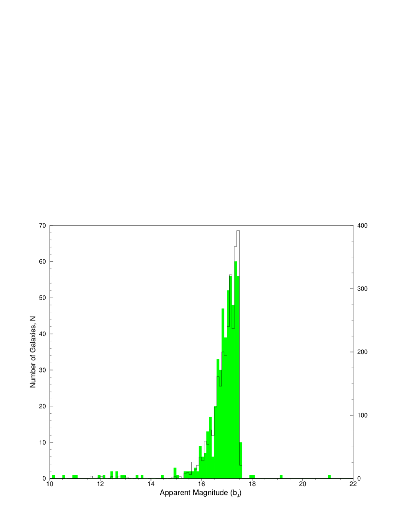
Figure 2: Histogram showing the magnitude distribution for the 6dF observations compared to the SuperCosmos inter-cluster galaxy list with limiting magnitude b${}_{J}=$ 17.5. Filled histogram shows the magnitude distribution of the observed objects (547) and correlates with the y-axis labeled on the left-hand side. Outlined histogram shows the original list of galaxies (2848) after the cluster galaxies were removed and correlates with the labels on the right-hand side.

Observations covering the 12°$\times$ 14° area in the HRS were carried out on the 1.2m UKST of the Anglo-Australian Observatory (AAO) in 2002 October/November. All observations were carried out as part of the 6dF Galaxy Survey (6dFGS) program being undertaken by the AAO (Wakamatsu et al., 2003). Specifically, the 6dFGS and our HRS program observations were folded together to allow for joint execution of both programs. When allocating fibers, the 1500 galaxies in the study were given highest priority within the 6dFGS for the selected fields of observation. However, whenever a 6dF fiber became unassigned due to a conflict with the fiber selection from another target galaxy, the fiber was then reassigned to a target from the 6dFGS lists. The blue magnitude limit for the 6dFGS is 16.75 (i.e., b${}_{J}<$ 16.75), hence there is considerable overlap between our target lists and the 6dFGS. Over all the observed fields, approximately 70% of all targets were taken from our original list of 1500 galaxies. Noticeable from Figure 2, our observed galaxy magnitude distribution closely follows the magnitude distribution of the post-extraction HRS area of 2848 galaxies. Due to the brighter limiting magnitude of 6dFGS, we have slightly less proportional coverage at our faint limit. In addition, a few very faint objects were included as part of the 6dFGS, which again can be seen in Figure 2. Finally, a small number of 6dFGS objects lie within our 1° excision radii around clusters, which is evident in Figure 1.

Observations and reductions were carried out along standard 6dFGS procedures, which are briefly summarized in the next section. Eight nights were allocated to this project by the 6dFGS team, but three were adversely affected by weather (Table 1). We used a combination of the 580V and 425R volume-phase holographic transmission gratings to optimize spectral coverage. This procedure yielded an instrumental resolution of 4.9 Å (580V) and 6.6 Å (425R), while covering the wavelength range 3900 $-$ 7600 Å, i.e., from [OII]$\lambda$3727 through H$\alpha$ over the HRS redshift range. Exposure times for each grating are listed in Table 1. HgCdNe arc and quartz flat exposures were carried out before and after primary fields.

2.3 Reductions

547 usable galaxy spectra were obtained from the eight nights allocated (Table 2). In Figure 1, individual field centers are labeled and shown in reference to the survey area. Altogether, 100 fibers were operational during our sequence of observations. With 9 fibers donated to sky, this leaves a total of 91 possible galaxy redshifts per imaged field. Night 7 with the 580V grating was not reduced due to a telescope focus error, so redshifts were obtained for only 25% of the 0811 field (Table 1). Although the signal-to-noise ratio was relatively low in many of our spectra ($<$ 10), over 95% yielded reliable redshifts (excluding 0811). Due to 6dFGS priorities and galaxy overcrowding, redshifts were obtained for some galaxies not originally included in our source lists. There remained 3 Galactic stars and 27 objects with unusable spectra in the sample.

The automatic 6dF data reduction (6DFDR) package completes the following steps directly after observation: debiasing, fiber extraction, cosmic-ray removal, flat fielding, sky subtraction, and wavelength calibration (Jones et al., 2004). As a final step, the post-6DFDR files from each exposure were co-added into single spectra.

2.4 Redshift Determination

Methods for the determination of galaxy redshifts fit into three basic categories depending on their spectral characteristics: absorption, emission, and those spectra containing both absorption and emission features. For spectra exhibiting absorption features, the IRAF based cross-correlation package, rvsao, was utilized to determine radial velocities against four template spectra: two stellar spectra obtained from the Coudé Feed spectral library (Jones, 1999) and two spectra obtained from the sample (a Galactic star and a nearby galaxy whose redshift was also determined by rvsao).

The method of determining redshifts for emission-dominated galaxy spectra was completed in two steps. First, JAR and MCF independently measured wavelength centers for each detectable spectral line via Gaussian fitting then determined its redshift. Second, each emission line was assigned a weight by MCF based upon the sharpness of the line and the surrounding noise level. The assigned weight was based upon a 5 point scale, where a “5” denoted a peak height greater than three times the FWHM with minimal background. For expected emission lines that were faintly detectable from the background, a weighting of “1” was assigned. This appropriately distinguished between emission lines with robust redshift determinations from those compromised by noise. Redshifts were averaged for galaxy spectra exhibiting both strong emission and absorption features. Whenever there was a discrepancy of $\Delta cz>100$ km s^-1 between the two methods, preference was given to the emission line value. As a last step, heliocentric corrections were applied to all redshifts.

2.5 Coverage

Outside the previously determined cluster areas that were excised, there were 2848 potential targets selected by SuperCOSMOS (galaxies with b${}_{J}<$ 17.5). It was determined from a comparable sub-sample selection that $\sim$15% of the targets labeled as ‘galaxies’ by SuperCOSMOS were actually stars. Therefore, the completeness of the survey is 547/2420, or 23%. The optical redshifts obtained in this survey more than double the previously published information regarding the proposed supercluster field (Figure 3). Previous inter-cluster observations were limited both spatially (primarily focused in the Southeast portion of the supercluster) and also by magnitude. Overlap with previously observed galaxies was not intended, but in general, most of the 6dF redshifts are consistent with previous estimates within the combined errors.

It is noticeable from Figure 1 that the coverage is not uniform over the original 12°$\times$ 14° area. In fact, the total area covered by the observations is more accurately 9°$\times$ 14°. Furthermore, the galaxies in the Western portion are more heavily sampled than those in the East. This non-uniformity is primarily a result of the weather problems coupled with the competing demands of both HRS and 6dFGS surveys when selecting field centers for the observations. Although the mean completeness is 23%, the field centers in the Western portion are sampled closer to 28% completeness, while the Eastern field centers are at $\sim$22%.

3 RESULTS

3.1 Kinematic Extent of the HRS

We begin by briefly considering the kinematic extent of the HRS. While a supercluster clearly will not be in a state of dynamical equilibrium with well-defined boundaries, we establish provisional kinematic limits from previous studies of the Horologium-Reticulum (HR) cluster population. Specifically, two separate studies applied a friends-of-friends analysis to the ACO clusters within the HR region and identified between 18 and 24 clusters as related to the HRS (Zucca et al., 1993; Einasto et al., 2001). Within our region of observation, seventeen ACO clusters were combined from these two catalogs (column 4, Table 3). The mean redshift of these clusters is 19,900 km s^-1, with a dispersion $\sigma$ of 2300 km s^-1. We define the “kinematic core” of the HRS to be roughly bounded by the FWHM of the observed redshift distribution of ACO clusters, namely 5400 km s^-1. When rounded to the nearest 500 km s^-1, we determine the core of the HRS to be between $cz$ of 17,000 and 22,500 km s^-1.

The above kinematic extent of $\sim$5500 km s^-1 is basically consistent with the fact that the Zucca et al. (1993) and Einasto et al. (2001) analyses find the HRS to contain $\sim$20 major galaxy clusters. Assuming a mean cluster mass of 10${}^{15}\,M_{\sun}$ and the cosmological parameters stated in §1, we calculate the spherical Hubble Flow volume required to contain a mass of 20 such clusters. The calculated diameter of that volume (95 Mpc) does indeed correspond to a velocity spread of $\sim$6500 km s^-1, i.e., similar to our defined kinematic limits.

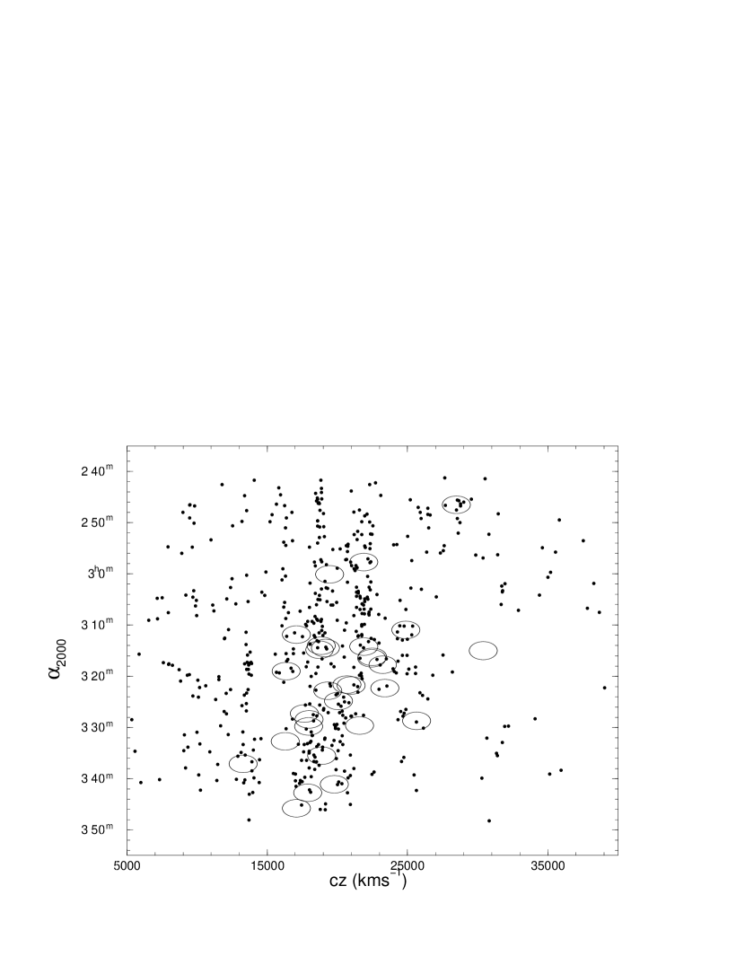
Figure 5: Coordinate-redshift plots for the 6dF galaxies. Left panel: $\alpha-cz$. Right panel: $\delta-cz$. Clusters in Figure 2 are shown as ellipses with an estimated velocity dispersion of 1000 km s^-1 (horizontal axis) and a vertical axis of 4 Mpc (2 R_A) at the mean HRS redshift (20,000 km s^-1).

The adopted boundaries for the HRS are examined with respect to both the distribution of cluster redshifts and the distribution of 6dF inter-cluster galaxy redshifts in Figure 4. For inset (a), all galaxy clusters with known redshifts in the region (Table 3) are plotted, including the seventeen ACO clusters considered above. Although the redshift histogram for the inter-cluster galaxies is clearly clumped into several redshift concentrations, the main concentration of galaxies ($\sim$48% of the sample) lies within the selected HRS kinematic boundaries. As shown in Figure 4(b), the HRS kinematic core is bordered by a depletion in galaxy numbers both at lower (14,000 $-$ 16,000 km s^-1) and higher (22,500 $-$ 24,000 km s^-1) redshift ranges. While the higher redshift limit to the HRS near cz = 22,500 km s^-1 is quite well defined, the lower redshift limit is less clearly defined. Specifically, there is a clump of galaxies present between 16,000 and 17,000 km s^-1, which is not included in our definition of the HRS “core”. The nature of the inter-cluster galaxies in this redshift regime is further clarified in Figure 5, where we plot coordinate versus redshift in both $\alpha$ and $\delta$. Note that the galaxies between 16,000 and 17,000 km s^-1 in redshift are highly concentrated in $\delta$ at $\sim-$54°. These same galaxies are more substantially spread in $\alpha$, although confined to the Western side of the HRS. We return to this component of the HRS in subsequent sections.

3.2 Inter-cluster Galaxy Overdensity

Our extensive new redshift database allows us to calculate the mean galaxy overdensity in the inter-cluster regions of the HRS. The expected galaxy counts for a uniform distribution are based on estimates of the local galaxy luminosity function (LF). To facilitate the comparison between the HRS and the SSC, we follow as closely as possible the methods described by Drinkwater et al. (2004). Specifically, the expected number of galaxy counts as a function of redshift and limiting magnitude are calculated from the same Metcalfe et al. (1991) galaxy LF as used by Drinkwater et al. (2004) in their calculation of the overdensity in the SSC. The resulting function is plotted as a solid curve in Figure 4, with an assumed limiting magnitude of b_J = 17.5. To calculate the expected number of galaxies within the HRS redshift and angular limits, we adopted the previously established redshift limits of 17000 $-$ 22500 km s^-1, and assumed the 9° $\times$ 14° = 126 deg² areal coverage of our survey. However, the latter figure required reduction to 107 deg², due to the areas excised around clusters. Finally, we observed only 23% of the total number of galaxies brighter than b_J of 17.5 within the 107 deg². Of the observed galaxies, $\sim$48% fall within the redshift limits of the HRS. Taking these factors into account, we arrive at a mean density of 2.4:1 for the inter-cluster regions of the HRS (assuming that light traces mass). In following a common definition of the galaxy overdensity, we find that $\bar{\delta}=$ 1.4, where $\bar{\delta}=(\rho_{HRS}-\bar{\rho})/{\bar{\rho}}$. Given the rather uncertain redshift and angular boundaries of the HRS, as well as uncertainty in the shape and normalization of the local LF, we estimate an uncertainty of $\sim$25% in the overdensity.

3.3 Large-Scale Redshift Trend

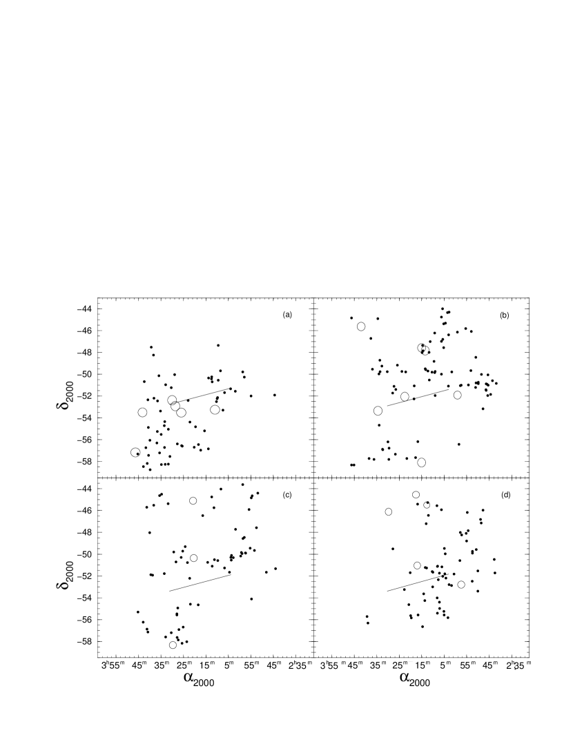
Figure 6: Redshift slices are plotted for the 6dF data in the range of the HRS. Each panel covers a 1500 km s^-1 redshift slice. Individual galaxies are plotted as small filled circles. Clusters from Figure 2 are also included in their respective redshift ranges. The short solid lines in each panel show the best-fit axis from the spatial-cz correlation analysis (PA$=-$80°). Only a short line is drawn because of the curvature produced by the non-equal area of the conventional $\alpha-\delta$ coordinate projection. Panel (a) 17,000 $-$ 18,500 km s^-1, Panel (b) 18,500 $-$ 20,000 km s^-1, Panel (c) 20,000 $-$ 21,500 km s^-1, Panel (d) 21,500 $-$ 23,000 km s^-1.

Having examined the overall redshift histograms for both clusters and inter-cluster galaxies, we now utilize two-dimensional redshift slices of our 6dF data as a further means of assessing the dynamical state of the HRS. In Figure 6, we present a sequence of redshift cuts through the kinematic extent of the HRS, each cut containing a redshift bin size of 1500 km s^-1. An examination of Figure 6 gives the impression of a systematic trend between spatial position in the HRS and redshift. Specifically, we note that galaxies in panel (a) (17,000 $-$ 18,500 km s^-1) appear preferentially located in the South and East, while the galaxies in panel (d) (21,500 $-$ 23,000 km s^-1) preferentially populate the West and North. In other words, there appears to be a trend of systematically increasing redshift along a principal axis in the HRS that extends from the Southeast to the Northwest end of the supercluster.

To quantify the significance of a large-scale redshift trend with spatial position in the HRS, we conducted a correlation analysis as a function of position angle (PA) on the sky. To begin, we selected the center of the HRS to be at ($\alpha=3^{h}16^{m},\delta=-52\arcdeg$) and assumed the principal axis of the HRS to be aligned along the West-East direction. Each galaxy was projected onto this principal axis, and we defined the S-coordinate to be the projected angular position of the galaxy along the assumed principal axis. Furthermore, the S-coordinate was defined to run negative to positive from West to East. A linear regression analysis was carried out between the redshift and the S-coordinate, which yields both the correlation coefficient, R, and the likelihood that the null hypothesis (no correlation between redshift and projected S position) is correct (Bevington 1969). We repeated the correlation analysis at 5° increments in position angle (PA) of the assumed principal axis over the full 180° range. When the assumed principal axis is running from SE to NW, positive S values are in the NW. In the same way, when the assumed principal axis is running from SW to NE, positive S values in the NE. The correlation analysis was completed both for the 263 6dF inter-cluster galaxies with redshifts between 17,000 and 22,500 km s^-1 and for the 21 clusters with mean redshifts over the same interval.

For both clusters and inter-cluster galaxies, we find that the null hypothesis is rejected at probability (P) levels of P$<1\%$. At certain PAs, the plots of $R$ versus PA show a broad peak over an interval of 20 $-$ 40°. 6dF galaxies show the highest correlation coefficient (R = 0.3) and lowest probability for the null hypothesis (P$<$10^-6) at a PA $\approx$ $-$80° (as measured East from North). The clusters also show a significant correlation, with a peak at a PA of $-$50°. In Figure 7, we show the projected S position plotted versus redshift for all inter-cluster galaxies and clusters with redshift between 17,000 and 22,500 km s^-1 at a PA of $-$80°. The expected cluster peculiar velocities are suppressed for clarity of the inter-cluster galaxy distribution. The linear regression fit for the inter-cluster galaxies is plotted as a solid line. Note that the best fit line actually passes through a zone of low galaxy density; this is examined further in §3.4.

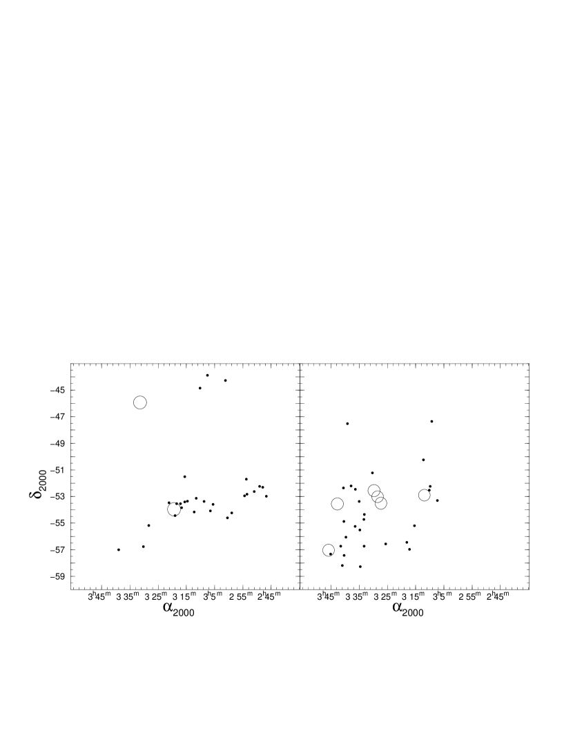
Figure 8: Separation of the 16000-18000 km s^-1 redshift slice into low- and high-redshift bins. The 16,000 $-$ 17,000 km s^-1 and 17,000 $-$ 18,000 km s^-1 galaxy populations are plotted in the left and right panels, respectively. Symbols as in Figure 3.

We are now in a position to revisit the substantial population of galaxies from 16,000 to 17,000 km s^-1. To determine whether or not these galaxies are associated with the large-scale redshift trend, we repeat the correlation analysis as a function of PA now expanding the redshift range to 16,000 $-$ 22,500 km s^-1. When the galaxies between 16,000 and 17,000 km s^-1 are included, the correlation coefficient is weakened (R = 0.2), and the probability of no correlation increases to P$\sim$10^-3. The deviation of the 16,000 $-$ 17,000 km s^-1 galaxies from the redshift trend is evident in their spatial segregation (especially in $\delta$). We display the spatial location of these galaxies on the sky in Figure 8, where the galaxies from 16,000 $-$18,000 km s^-1 are separated into 1000 km s^-1 slices. Although the galaxies from 16,000 $-$17,000 km s^-1 only represent $\sim$5% of the total population, the spatial segregation of this clump does not follow the overall trend of the higher redshift galaxies in the HRS and provides a significant lever arm by which the best fit correlation axis is altered. In short, while the spatially-localized galaxies from 16,000 $-$ 17,000 km s^-1 may reside within the HRS, they do not appear to follow the large-scale redshift trend established by the clusters and inter-cluster galaxies over the range 17,000 $-$ 22,500 km s^-1.

3.4 Bi-Modal Kinematics of the HRS

As noted above, the best linear fit between projected S coordinate and redshift actually runs through a zone of low galaxy density (Figure 7). The implication is that the HRS has a bi-modal redshift distribution, i.e., the HRS kinematic extent consists of two major components in redshift. The redshift bi-modality of the HRS is most clearly observed by fitting and removing the systematic spatial-redshift trend at PA $=-$80°, then plotting the histogram of residual redshifts, as shown in Figure 9. Fitting each component of the histogram with a Gaussian reveals that the overall number of galaxies is roughly equal in the two components, which are separated by $\sim$2500 km s^-1 (35 Mpc). However, the FWHM of the higher-redshift component (i.e., corresponding to the galaxies with original redshift centered at $\sim$21,000 km s^-1) is approximately twice as large as for the lower redshift component, 2200 and 1100 km s^-1, respectively. Furthermore, the two components show no spatial distinction from each other and are spread throughout the entire observed region of the HRS.

To quantify the likelihood of bi-modality in the redshift distribution, we first assess the likelihood that a single Gaussian provides an adequate fit to the data. At each PA, we determine the residual redshift of all galaxies from the systematic position-redshift trend, and then we employ KMM statistics to assess the likelihood of a two-Gaussian versus a single-Gaussian fit (Ashman et al., 1994). For all position angles, a common covariance, two-Gaussian fit is preferred to a single Gaussian with a high degree of confidence ($>$ 99%). The average peak-to-peak separation of the two components over the entire PA range is 3014 $\pm$ 712 km s^-1, with the separation along the best-fit line (PA$=-$80°) being 3003 $\pm$ 174 km s^-1. Next, we utilize $\chi^{2}$ statistics to test the goodness-of-fit for two Gaussian distributions with differing FWHM as a function of PA. The reduced $\chi^{2}$ values range from 0.95 to 4.91 with the best fit value at PA$=-$60°. In summary, the statistical tests confirm the bi-modal nature of the HRS redshift distribution, with the clearest distinction between the two redshift components occurring along the principal spatial-redshift axis of the supercluster.

Finally, we have utilized the same KMM statistical methods to assess the redshift distribution of clusters in the HRS with known redshift. For the clusters, the best fit correlation axis was found at PA$=-$50°. However when considering the broad nature of the correlation$-$PA relationship for clusters, we used the best fit line from the inter-cluster galaxies at a PA of $-$80° (cf., Figure 7). We fitted the systematic position-redshift trend of the galaxies and found the residual mean redshift for each cluster from that trend. The resulting histogram of cluster residual redshift was plotted in Figure 9 (right). We then applied KMM statistics to the cluster histogram. Unlike the test on the galaxies, the cluster histogram showed no clear signature of a bi-modal redshift distribution. Specifically, the cluster redshifts fitted a bi-modal distribution with $\sim$75% confidence as compared to a single Gaussian distribution. However, as can be seen in Figure 9 (right), the cluster redshift data were sparse and little could be concluded from their redshift distribution.

4 Comparisons with the Shapley Concentration

The HRS is generally referred to as the second largest supercluster within 200 Mpc, second only in mass to the Shapley Supercluster (SSC) (Hudson et al., 1999). Since the SSC is both well-studied and the most comparable supercluster in the local universe, we use it as a benchmark for assessing the properties of the HRS. The comparison between these two largest structures is somewhat hindered by the fact that most of the SSC studies combine inter-cluster and cluster galaxies, while our 6dF data for the HRS samples only the inter-cluster galaxies.

4.1 Extent and Overdensity

We begin by comparing the kinematic extent of the HRS (from 17,000 to 22,500 km s^-1) with that of the SSC. The velocity boundaries of the entire SSC are generally cited as extending from 8,000 to 18,000 km s^-1 (Quintana et al., 2000; Drinkwater et al., 2004). To put the SSC on the same quantitative footing as the HRS, we compare the cluster populations of the two superclusters. Specifically, when compared with the 18 ACO clusters found in the HRS by Zucca et al. (1993), the same authors find 24 ACO clusters in the SSC, while Einasto et al. (2001) find 25. Hence the numbers of clusters in the SSC are comparable to, perhaps slightly larger than, those in the HRS. For the 24 ACO clusters combined from these studies, we used published mean redshift data from Quintana et al. (2000) to calculate a comparative kinematic extent for the SSC. We determine the FWHM of the redshift distribution of the SSC clusters to be $\sim$6000 km s^-1, very similar to the $\sim$5500 km s^-1 found for the HRS. As is discussed below, the redshift distribution of the SSC clusters is distinctly bi-modal, thus the FWHM metric is rather an oversimplification of a complex environment. However, the basic result is that the HRS and SSC are similar in regard to their total number of ACO clusters and overall kinematic extent.

Next, we seek to make a valid comparison between the inter-cluster overdensities of the SSC and the HRS. Three studies have examined in detail the inter-cluster overdensity of the SSC (Drinkwater et al., 1999; Bardelli et al., 2000; Drinkwater et al., 2004). Of these, only Drinkwater et al. (2004) considers a similar area on the sky, so we draw a comparison with this study. The SSC inter-cluster overdensity is 3.3 $\pm$ 0.1 over 151 deg², as compared with an overdensity of 2.4 that we find for the HRS. A radius of 0.5° ($\sim$ 2 Mpc at SSC mean redshift) was excised around ACO clusters within the survey area. This radius in the SSC corresponds to 0.35° at the HRS redshift. Consequently, the HRS sample is slightly more restrictive in selecting only inter-cluster galaxies, but this is likely a small difference. Overall, we find a somewhat smaller, but similar, overdensity in the HRS compared to that in the SSC.

In addition, we compare the total mass in the HRS inter-cluster galaxies to that in the SSC. Given the differences between the HRS and SSC studies in overdensity (2.4/3.3), angular survey region (107/151 deg²), and relative distance ($\sim$ 20,000/15,000 km s^-1), we conclude that the total masses of the inter-cluster regions of the HRS and SSC are virtually identical. Thus our data indeed support the conclusion of previous studies of the distribution of galaxy clusters (Zucca et al., 1993; Hudson et al., 1999; Einasto et al., 2001) that the SSC and HRS constitute the two largest mass concentrations in the local universe.

4.2 Morphological Considerations

In §3.2, we found an overall spatial-redshift trend in the HRS, in that a systematic increase in redshift is present with increasing position along a SE$-$NW axis. Bardelli et al. (2000) have fitted a plane in ($\alpha$, $\delta$, $cz$) space to their inter-cluster observations in the SSC. They note a $\sim$3000 km s^-1 increase in average galaxy velocity along the best fit plane over the 8° (40 Mpc) region, a result reminiscent of the position-redshift tilt in the HRS. However, when the area on the sky is expanded (cf., Figure 4 of Bardelli et al., 2000) to include the inter-cluster galaxies in Drinkwater et al. (1999), the main peak of the galaxy distribution shifts by 7 Mpc, and the entire distribution is broadened. In short, while there appears to be a kinematic gradient in the SSC, it is not clear whether that feature extends over the entire region of the supercluster.

As is discussed in §3.3, when the spatial-redshift trend along the PA=$-$80° axis in the HRS is fitted and removed, the redshift distribution is bi-modal (Figure 9). In fact, the bi-modal signature is observed even in the original redshift histogram in Figure 4. Redshift bi-modality is also strikingly evident in the SSC (cf., Figure 6 of Drinkwater et al., 2004; Quintana et al., 2000, Figure 5). There is a lower redshift component to the SSC (at $\sim$8,000 $-$ 12,000 km s^-1) that is quite distinct from the higher component at $\sim$14,000 $-$ 18,000 km s^-1. While it was originally thought that the SSC redshift components are substantially different in size, an extensive follow-up study by Drinkwater et al. (2004) reveals the inter-cluster populations of the two components to be roughly equal (cf., Figure 5 of Drinkwater et al., 2004). On the other hand, the distribution of the clusters within the SSC is also bi-modal and more heavily weighted to the higher redshift component at 13,000 $-$ 18,000 km s^-1. Specifically, 16 clusters have redshifts above 13,500 km s^-1, while only 6 have redshifts below 12,500 km s^-1. The higher redshift component coincides with what is designated by Reisenegger et al. (2000) as the collapsing “Central Region,” centered on the cluster A3558. As a result, the higher redshift component dominates when both the cluster and inter-cluster galaxies are considered. More reliable redshift data for the clusters in the HRS is probably required before a definitive statement can be made about their redshift distribution, but the available data (cf., Figure 9, Right panel) indicate that such a 3:1 imbalance in cluster numbers between lower and higher redshift components is not present.

Although our observations reveal a distinct arrangement of field galaxies marking the HRS, the extent and/or boundaries of the supercluster are not easily determined. In fact, percolation and friends-of-friends algorithms include other clusters in the HRS besides those listed in Table 3 (Kalinkov et al., 1998; Einasto et al., 2002). Recent studies of the SSC cover a similar area on the sky and also leave some ambiguity as to the spatial and kinematic extent of the supercluster (Quintana et al., 2000; Drinkwater et al., 2004). It is quite possible that the boundaries of the HRS extend beyond the region surveyed by us with 6dF.

5 CONCLUSIONS

We have obtained optical redshift data for 547 inter-cluster galaxies in the region of the Horologium-Reticulum Supercluster (HRS). This extensive coverage of the inter-cluster galaxies provides an opportunity to define large-scale kinematic structures within the HRS. Our initial result is the detection of a main concentration of inter-cluster galaxies from 17,000 $-$ 22,500 km s^-1, which we refer to as the HRS kinematic extent. This was followed by the comparison of our observations with a smooth, homogeneous galaxy distribution. An overdensity of 2.4 was calculated, or $\delta\rho/\bar{\rho}\sim$ 1.4, which reveals that the HRS complex has entered the non-linear regime. Through visual inspection of redshift slices, reinforced with correlation analysis, the galaxies within the kinematic extent are found to exhibit a significant trend in redshift with position along a SE$-$NW axis in the sense that redshift increases by $\sim$1500 km s^-1 along this axis. Furthermore, the resulting position angle of the trend is closely aligned with that found in the clusters within the HRS. In addition, when the kinematic trend found above is accounted for and removed, we find a distinct bi-modality to the redshift distribution of the inter-cluster galaxies within the HRS. Thus, the HRS can be viewed as consisting of two major components in redshift space, separated by 2500 km s^-1 (35 Mpc), each with a similar position-redshift tilt at the same position angle.

We thank Fred Watson, Paul Cass, and the 6dFGS team for supervising and conducting our observations, as well as Keith Ashman for his quick response with the KMM code. We also thank Rien van de Weygaert and Saleem Zaroubi at the Kapteyn Institute, Groningen, NL for helpful discussions. We acknowledge useful comments from the referee, which led to considerable improvements in the final paper. MCF acknowledges the support of a NASA Space Grant Graduate Fellowship at the University of North Carolina-Chapel Hill. RWH acknowledges grant support from the Australian Research Council. A portion of this work was supported by NSF grants AST-9900720 and AST-0406443 to the University of North Carolina-Chapel Hill.

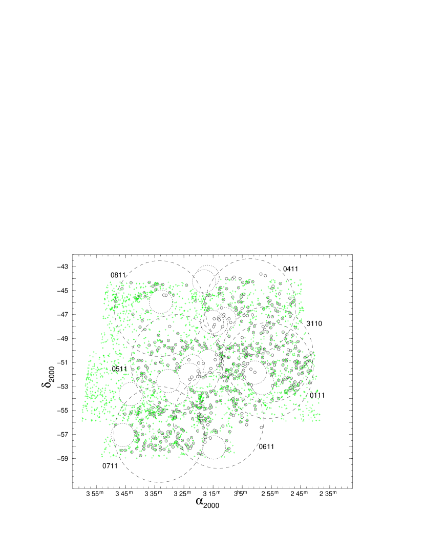
Figure 1: Observed fields in the present study as conducted by the 6dFGS team. Crosses represent all 2848 galaxies from the SuperCOSMOS catalog. Note that, as described in the text, one degree radius regions ($\sim$2 R_A) around 16 ACO clusters listed as members of the HRS by Zucca et al. (1993) are excluded from the catalog. The excised regions are shown as dotted circles. Small, open circles represent galaxies for which optical redshifts were obtained. The 6dF r$-\theta$ positioner selects a 6-degree diameter region from the UKST field plates, which are denoted by large dashed circles. Labels refer to the spectroscopic observations detailed in Table 1 (column 4).

Figure 3: The HRS region under study displaying both 6dF and previous inter-cluster redshifts. Previously observed galaxies are plotted with different symbols to show the increased amount of information with our 6dF study. Redshifts from our 2002 study are shown as filled circles. Clusters in the observing region with known redshift (Table 3) are shown as large open circles with radii of 2 Mpc (1 R_A).

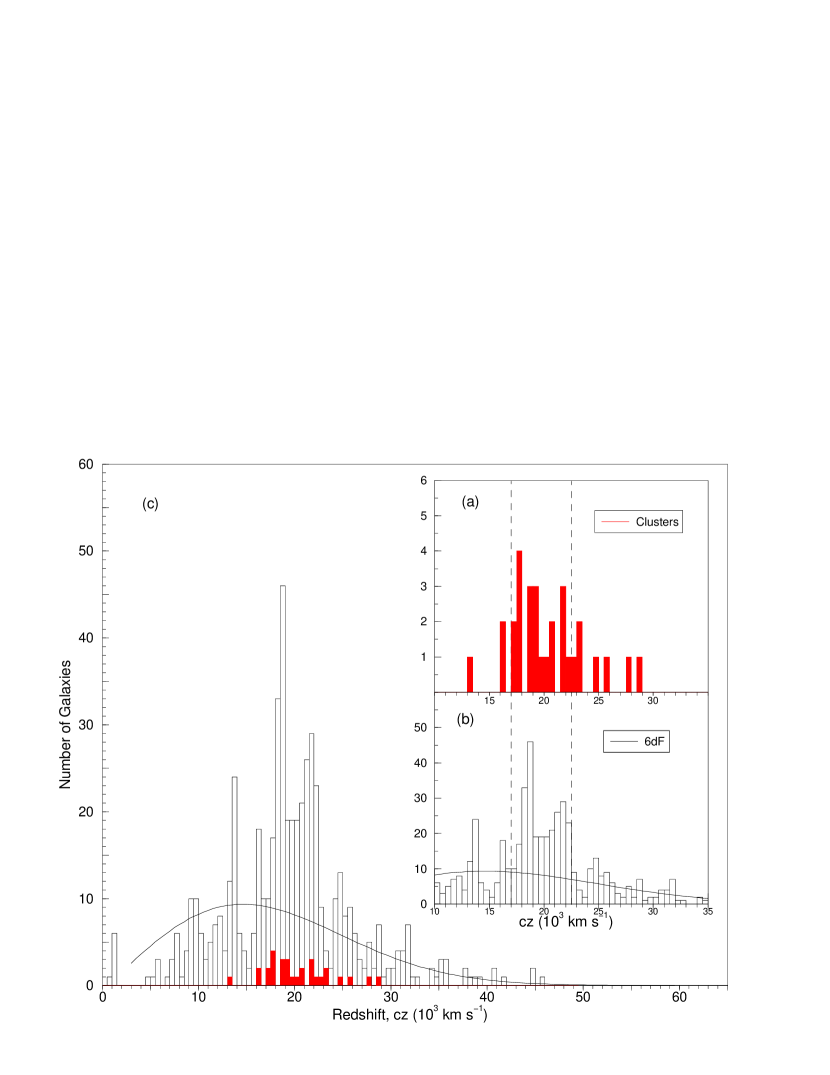
Figure 4: Redshift histograms of the 6dF inter-cluster galaxies (open) and the clusters with known redshifts (filled). Panel (a): Cluster redshifts from Table 3. Panel (b): Redshifts for inter-cluster galaxies covering the same range as clusters in panel (a). Dashed lines in both inset histograms represent the kinematic “core” discussed in the text. In panel (c), we show the entire redshift histogram for the inter-cluster galaxies with the clusters overlaid. Solid line shown in both inter-cluster galaxy histograms is the expected number of counts for a smooth, homogeneous distribution. The redshift bin size is 500 km s^-1.

Figure 7: Projected angular S-coordinate (see text) is plotted versus redshift for 6dF galaxies between 17,000 and 22,500 km s^-1. The position angle (PA) of the principal axis of projection is at $-$80° (as measured East from North), with positive S values in the NW. Individual galaxies are plotted as small filled circles, while open circles represent clusters in the region. The best fit linear regression is plotted as a solid line.

Figure 9: Residual redshift histograms for galaxies and clusters within 17,000 $-$ 22,500 km s^-1. The residual redshift is measured relative to the linear regression line that represents the best fit between projected S coordinate and redshift for an assumed principal axis oriented at PA$=-$80°, i.e., the best fit line in Figure 8. Left panel: 6dF galaxies, 250 km s^-1 bin size ; Right panel: Clusters of known redshift, 500 km s^-1 bin size.

Table 1: Spectroscopic Observations

Date	$\alpha_{2000}$	$\delta_{2000}$	ID	Field No.	Grating	texp(s)	Seeing	S/N
2002 Oct 31	02 55 57.9	$-$50 18 20	3110	198,199	580V	4$\times$1200	2$-$3″	7.5
				154	425R	4$\times$600	3$-$5″	9.0
2002 Nov 01	02 55 57.9	$-$51 38 12	0111	198,199	580V	4$\times$1200	1$-$2″	9.0
				154	425R	4$\times$600	1$-$2″	11.7
2002 Nov 03	03 02 00.4	$-$46 18 17	0411	247, 248	580V	4$\times$600	3$-$5″	4.6
2002 Nov 04	03 02 00.5	$-$46 18 15	0411	247, 248	425R	4$\times$600	2$-$3″	10.8
					580V	4$\times$1200	3$-$4″	8.7
2002 Nov 05	03 24 57.6	$-$50 58 17	0511	200	425R	4$\times$600	2$-$3″	12.6
					580V	4$\times$1200	2.2″	9.8
2002 Nov 06	03 17 55.5	$-$55 48 06	0611	155	425R	4$\times$600	2$-$3″	10.8
					580V	4$\times$1200	3$-$4″	7.8
2002 Nov 07	03 28 54.8	$-$56 58 04	0711	155, 156	425R	4$\times$600	1$-$2″	10.5
					580V	6$\times$1200	3$-$4″, cloudy	8.6
2002 Nov 08	03 33 02.2	$-$46 28 04	0811	200, 248	425R	4$\times$600	1$-$2″	5.4
				249	580V	4$\times$1200	1$-$2″	$-$

Note. — Numbers in parentheses refer to the column numbers. (1) Date of observation, (2) Right Ascension of the field center in hours, minutes, and seconds (J2000), (3) Declination of the field center in degrees, arcminutes, and arcseconds (J2000), (4) Identification number as found in Figure 1, (5) Schmidt field number, (6) Grating, (7) Exposure time, (8) Approximate seeing, (9) Average signal-to-noise.

Table 2: Velocity Data for 6dF Galaxy Spectra

ID	$\alpha_{2000}$	$\delta_{2000}$	bJ	Reference	$cz$ (km s-1)	$\sigma_{cz}$
HRS J024113$-$501154	02 41 13.42	$-$50 11 54.1	13.41	e	27662	40
HRS J024126$-$514012	02 41 26.02	$-$51 40 12.0	17.36	e	30523	86
HRS J024141$-$524151	02 41 41.38	$-$52 41 51.7	17.17	e	14078	52
HRS J024141$-$505106	02 41 41.86	$-$50 51 06.1	16.93	e	18818	47
HRS J024213$-$514333	02 42 13.22	$-$51 43 33.2	17.45	e	22710	50
…	…	…	…	…	…	…

Note. — Numbers in parentheses refer to the column numbers. (1) IAU name, (2) Right ascension in hours, minutes, and seconds (J2000), (3) Declination in degrees, arcminutes, and arcseconds (J2000), (4) b_J magnitude as listed in SuperCOSMOS, (5) “a”= absorption lines used to calculate redshift, “e”= emission lines used to calculate redshift, “ae”= both absorption and emission lines used, (6) Velocity, $cz$, (7) Velocity error. The complete version of this table is in the electronic edition of the Journal. The printed edition contains only a sample.

Table 3: Clusters of Known Redshift in the Observed Region

Cluster	$\alpha_{2000}$	$\delta_{2000}$	List	Redshift	cz (km s-1)	Source
A3047	02 45.2	$-$46 27.0		0.0950	28500	1
A3074	02 57.9	$-$52 43.0	B	0.0730	21900	1
A3078	03 00.5	$-$51 50.0	B	0.0648	19440	2
A3093	03 10.9	$-$47 23.0	B	0.0830	24900	2
M031027	03 11.9	$-$52 54.0		0.0570	17088	1
A3100	03 13.8	$-$47 47.0	B	0.0629	18870	2
A3104	03 14.3	$-$45 24.0	B	0.0730	21900	1
A3106	03 14.5	$-$58 05.0	B	0.0639	19170	2
A3108	03 15.2	$-$47 37.0	B	0.0625	18750	3
A3109	03 16.7	$-$43 51.0	B	0.0920	27580	3
A3110	03 16.5	$-$50 54.0	B	0.0749	22470	2
A3111	03 17.8	$-$45 44.0	E	0.0775	23250	4
A3112	03 17.9	$-$44 14.0	B	0.0750	22500	4
S0339	03 19.0	$-$53 57.4		0.0546	16369	1
S0345	03 21.8	$-$45 32.3		0.0700	20985	1
A3120	03 21.9	$-$51 19.0	B	0.0690	20700	2
M391	03 22.3	$-$53 11.3		0.0780	23384	1
A3123	03 23.0	$-$52 01.0	B	0.0644	19320	2
M03233	03 24.8	$-$58 35.1		0.0670	20086	1
A3125	03 27.4	$-$53 30.0	B	0.0589	17670	5
M399	03 28.4	$-$53 01.3		0.0600	17988	1
A3126	03 28.7	$-$55 42.0		0.0856	25680	4
S0356	03 29.6	$-$45 58.8		0.0720	21585	1
A3128	03 30.2	$-$52 33.0	B	0.0599	17970	4
A3133	03 32.7	$-$45 56.0	B	0.0543	16290	2
M421	03 35.5	$-$53 40.9		0.0630	18887	1
A3144	03 37.1	$-$55 01 0		0.0443	13290	2
M433	03 41.1	$-$45 41.5		0.0660	19786	1
A3158	03 43.0	$-$53 38.0	B	0.0597	17910	4
A3164	03 45.8	$-$57 02.0	B	0.0570	17100	2

Note. — Numbers in parentheses apply to column numbers. (1) A-ACO, S-poor clusters from ACO, M- APM Galaxy Survey; (2) Right Ascension in hours and minutes (J2000); (3) Declination in degrees and minutes (J2000); (4) B-HRS membership listed in both Zucca et al. (1993) and Einasto et al. (2001), E-HRS membership listed only in Einasto et al. (2001); (7) ¹Dalton et al. (1994), ²Struble & Rood (1999), ³den Hartog (1995), ⁴Katgert et al. (1998), ⁵Caldwell & Rose (1997).

References

- Abell, Corwin & Olowin (1989) Abell, G. O., Corwin, H. G., Jr., & Olowin, R. P. 1989, ApJS, 70, 1
- Ashman et al. (1994) Ashman, K. M., Bird, C. M., & Zepf, S. E. 1994, AJ, 108, 6
- Barmby & Huchra (1998) Barmby, P. & Huchra, J. P. 1998, AJ, 115, 6
- Bardelli et al. (2000) Bardelli, S., Zucca, E., Zamorani, G., Moscardini, L., & Scaramella, R. 2000, MNRAS, 312, 3
- Baugh et al. (2000) Baugh, C. M., et al. 2000, MNRAS, 351, L44
- Bevington (1969) Bevington, P. R. 1969, Data Reduction & Error Analysis for the Physical Sciences, 1st ed., New York: McGraw-Hill
- Caldwell & Rose (1997) Caldwell, N. & Rose J. A. 1997, AJ, 113, 492
- Chamaraux et al. (1990) Chamaraux, P., Cayatte, V., Balkowski, C., & Fontanelli, P. 1990, A&A, 229, 340
- Chincarini et al. (1984) Chincarini, G., Tarenghi, M., Sol, H., Crane, P., Manousoyannaki, I., & Materne, J. 1983, A&AS, 57, 1
- Dalton et al. (1994) Dalton, G. B., Efstathiou, G., Maddox, S. J., & Sutherland, W. J. 1994, MNRAS, 269, 151
- de Lapparent, Geller, & Huchra (1986) de Lapparent, V., Geller, M. J., & Huchra, J. P. 1986, ApJL, 302, L1
- den Hartog (1995) den Hartog, R. 1995, Ph.D. thesis, University of Leiden.
- Drinkwater et al. (2004) Drinkwater, M. J., Parker, Q. A., Quentin A., Proust, D., Slezak, E., & Quintana, H. 2004, PASA, 21,89
- Drinkwater et al. (1999) Drinkwater, M. J., Proust, D., Parker, Q. A., Quintana, H., & Slezak, E. 1999, PASA, 16, 2
- Einasto et al. (2001) Einasto, M., Einasto, J., Tago, E., Muller, V., & Andernach, H. 2001, 123, 51
- Einasto et al. (2002) Einasto, M., Einasto, J., Tago, E., Andernach, H., Dalton, G. B., & Muller, V. 2002, 123, 51
- Gregory & Thompson (1978) Gregory, S. A. & Thompson, L. A. 1978, ApJ, 222, 784
- Hambly et al. (2001) Hambly, N. C., et al. 2001, MNRAS, 326, 4
- Haynes & Giovanelli (1986) Haynes, M. P. & Giovanelli, R. 1986, ApJL, 306, L55
- Hudson et al. (1999) Hudson, M. J., Smith, R. J., Lucey, J. R., Schlegel, D. J., & Davies, R. L. 1999, ApJ, 512, L79
- Jones (1999) Jones, L. A. 1999, Ph.D. thesis, University of North Carolina
- Jones et al. (2004) Jones, D. H., et al. 2004, MNRAS, 355, 747
- Kalinkov et al. (1998) Kalinkov, M., Valtchanov, I., & Kuneva, I. 1998, ApJ, 506, 509
- Katgert et al. (1998) Katgert, P., et al. 1998, A&AS, 129, 399
- Loveday et al. (1996) Loveday, J., Peterson, B. A., Maddox, S. J., & Efstathiou, G. 1996, ApJS, 107, 201
- Lucey et al. (1983) Lucey, J. R., Dickens, R. J., Mitchell, R. J., & Dawe, J. A. 1983, MNRAS, 203, 545
- Metcalfe et al. (1991) Metcalfe, N., Shanks, T., Fong, R., & Jones, L. R. 1991, MNRAS, 249, 498
- Motl et al. (2004) Motl, P. M., Burns, J. O., Loken, C., Norman, M. L., & Bryan, G. 2004, ApJ, 606, 635
- Novikov et al. (1999) Novikov, D. I., Melott, A. L., Wilhite, B. C., Kaufman, M., Burns, J. O., Miller, C. J., & Batuski, D. J. 1999, MNRAS, 304, 1
- Parker et al. (1998) Parker, Q. A., Watson, F. G., & Miziarski, S. 1998, in ASP Conference Series 152, Fiber Optics in Astronomy III, ed. S. Arribas, E. Mediavilla & F. Watson, 80
- Quintana et al. (2000) Quintana, H., Carrasco, E. R., & Reisenegger, A. 2000, AJ, 120, 511
- Reisenegger et al. (2000) Reisenegger, A., Quintana, H., Carrasco, E. R., & Maze, J. 2000, AJ, 120, 523
- Rose et al. (2002) Rose, J. A., Gaba, A. E., Christiansen, W. A., Davis, D. S., Caldwell, N., Hunstead, R. W., & Johnston-Hollitt, M. 2002, AJ, 123, 3
- Shapley (1935) Shapley, H. 1935, Ann. Harvard Coll. Obs., 88, 105
- Struble & Rood (1999) Struble, M. F. & Rood, H. J., 1999, ApJS, 125, 35
- Tully et al. (1992) Tully, R. B., Scaramella, R., Vettolani, G., & Zamorani, G. 1992, ApJ, 388, 9
- Wakamatsu et al. (2003) Wakamatsu, K., Colless, M., Jarrett, T., Parker, Q., Saunders, W., & Watson, F. 2003, in ASP Conference Proceedings 289, IAU 8th Asian-Pacific Regional Meeting, 1, ed. S. Ikeuchi, J. Hearnshaw & T. Hanawa (San Francisco: ASP), 97
- West, Jones, & Forman (1995) West, M. J., Jones, C., & Forman, W. 1995, ApJL, 451, L5
- Zucca et al. (1993) Zucca, E., Zamorani, G., Scaramella, R., & Vettolani, G. 1993, ApJ, 407, 2