On the role of injection in kinetic approaches to nonlinear particle acceleration at non-relativistic shock waves

Abstract

The dynamical reaction of the particles accelerated at a shock front by the first order Fermi process can be determined within kinetic models that account for both the hydrodynamics of the shocked fluid and the transport of the accelerated particles. These models predict the appearance of multiple solutions, all physically allowed. We discuss here the role of injection in selecting the real solution, in the framework of a simple phenomenological recipe, which is a variation of what is sometimes referred to as thermal leakage. In this context we show that multiple solutions basically disappear and when they are present they are limited to rather peculiar values of the parameters. We also provide a quantitative calculation of the efficiency of particle acceleration at cosmic ray modified shocks and we identify the fraction of energy which is advected downstream and that of particles escaping the system from upstream infinity at the maximum momentum. The consequences of efficient particle acceleration for shock heating are also discussed.

1 Introduction

Diffusive particle acceleration at non-relativistic shock fronts is an extensively studied phenomenon. Detailed discussions of the current status of the investigations can be found in some excellent reviews (Drury 1983; Blandford & Eichler 1987; Berezhko & Krimsky 1988; Jones & Ellison 1991; Malkov & Drury 2001). While much is by now well understood, some issues are still subjects of much debate, for the theoretical and phenomenological implications that they may have. One of the most important of these is the reaction of the accelerated particles on the shock: the violation of the test particle approximation occurs when the acceleration process becomes sufficiently efficient that the pressure of the accelerated particles is comparable with the incoming gas kinetic pressure. Both the spectrum of the particles and the structure of the shock are changed by this phenomenon, which is therefore intrinsically nonlinear.

At present there are three viable approaches to determine the reaction of the particles upon the shock: one is based on the ever-improving numerical simulations (Jones & Ellison 1991; Bell 1987; Ellison, Möbius & Paschmann 1990; Ellison, Baring & Jones 1995, 1996; Kang & Jones 1997; Kang, Jones & Gieseler 2002; Kang & Jones 2005) that allow one to achieve a self-consistent treatment of several effects.

The second approach is based on the so-called two-fluid model, and treats cosmic rays as a relativistic second fluid. This class of models was proposed and discussed in (Drury & Völk 1980, 1981; Drury, Axford & Summers 1982; Axford, Leer & McKenzie 1982; Duffy, Drury & Völk 1994). These models allow one to obtain the thermodynamics of the modified shocks, but do not provide information about the spectrum of accelerated particles.

The third approach is semi-analytical and may be very helpful to understand the physics of the nonlinear effects in a way that sometimes is difficult to achieve through simulations, due to their intrinsic complexity and limitations in including very different spatial scales. Blandford (1980) proposed a perturbative approach in which the pressure of accelerated particles was treated as a small perturbation. By construction this method provides the description of the reaction only for weakly modified shocks.

Alternative approaches were proposed by Eichler (1984), Ellison & Eichler (1984), Eichler (1985) and Ellison & Eichler (1985), based on the assumption that the diffusion of the particles is sufficiently energy dependent that different parts of the fluid are affected by particles with different energies. The way the calculations are carried out implies a sort of separate solution of the transport equation for subrelativistic and relativistic particles, so that the two spectra must be somehow connected at $p\sim mc$ a posteriori.

In (Berezhko, Yelshin & Ksenofontov 1994; Berezhko, Ksenofontov & Yelshin 1995; Berezhko 1996) the effects of the non-linear reaction of accelerated particles on the maximum achievable energy were investigated, together with the effects of geometry. The maximum energy of the particles accelerated in supernova remnants in the presence of large acceleration efficiencies was also studied by Ptuskin & Zirakashvili (2003a,b).

The need for a practical solution of the acceleration problem in the non-linear regime was recognized by Berezhko & Ellison (1999), where a simple analytical broken-power-law approximation of the non-linear spectra was presented.

Recently, some promising analytical solutions of the problem of non-linear shock acceleration have appeared in the literature (Malkov 1997; Malkov, Diamond & Völk 2000; Blasi 2002, 2004). Blasi (2004) considered for the first time the important effect of seed pre-existing particles in the acceleration region (the linear theory of this phenomenon was first studied by Bell (1978)). In a recent work by Kang & Jones (2005) the seed particles were included in numerical simulations of the acceleration process.

Numerical simulations have been instrumental to identify the dramatic effects of the particles reaction: they showed that even when the fraction of particles injected from the thermal gas is relatively small, the energy channelled into these few particles can be an appreciable part of the kinetic energy of the unshocked fluid, making the test particle approach unsuitable. The most visible effects of the reaction of the accelerated particles on the shock appear in the spectrum of the accelerated particles, which shows a peculiar hardening at the highest energies. The analytical approaches reproduce well the basic features arising from nonlinear effects in shock acceleration.

There is an important point which is still lacking in the calculations of the non-linear particle acceleration at shock waves, namely the possible amplification of the background magnetic field, found in the numerical simulations by Lucek & Bell (2000, 2000a) and Bell & Lucek (2001) and recently described by Bell (2004). This effect is still ignored in all calculations of the reaction of cosmic rays on the shock structure. We will not include this effect in the present paper.

Nonlinear effects in shock acceleration of thermal particles result in the appearance of multiple solutions in certain regions of the parameter space. This phenomenon is very general and was found in both the two-fluid models (Drury & Völk 1980, 1981) and in the kinetic models (Malkov 1997; Malkov et al. 2001; Blasi 2004). Monte Carlo approaches do not show multiple solutions.

This behaviour resembles that of critical systems, with a bifurcation occurring when some threshold is reached in a given order parameter. In the case of shock acceleration, it is not easy to find a way of discriminating among the multiple solutions when they appear. In (Mond & Drury 1998), a two fluid approach has been used to demonstrate that when three solutions appear, the one with intermediate efficiency for particle acceleration is unstable to corrugations in the shock structure and emission of acoustic waves. Plausibility arguments may be put forward to justify that the system made of the shock plus the accelerated particles may sit at the critical point (see for instance the paper by Malkov, Diamond & Völk (2000)), but we are not aware of any real proof that this is what happens. The physical parameters that play a role in this approach to criticality are the maximum momentum achievable by the particles in the acceleration process, the Mach number of the shock, and the injection efficiency, namely the fraction of thermal particles crossing the shock that are accelerated to nonthermal energies. The last of them, the injection efficiency, hides a crucial physics problem by itself, and plays an important role in establishing the level of shock modification. This efficiency parameter in reality is determined by the microphysics of the shock and should not be a free parameter of the problem. Unfortunately, our poor knowledge of such microphysics, in particular for collisionless shocks, does not allow us to establish a clear and universal connection between the injection efficiency and the macroscopic shock properties. Put aside the possibility to have a fully self-consistent picture of this phenomenon, one can try to achieve a phenomenological description of it. Kang, Jones & Gieseler (2002) introduced a sort of weight function to determine a return probability of particles in the downstream fluid to the upstream fluid, as a function of particle momentum. Only sufficiently suprathermal particles can jump back to the upstream region and therefore take part in the acceleration process. Here we adopt an injection recipe which is similar to the thermal leakage model of Kang et al. (2002) (see also previous papers by Malkov (1998) and by Gieseler et al. (2000)) and implement it in the semi-analytical approach of Blasi (2002, 2004). We investigate then the phenomenon of multiple solutions and show that the injection recipe dramatically reduces the appearance of these situations. We also study in some detail the efficiency for particle acceleration as a function of the Mach number of the shock and the maximum momentum of the accelerated particles.

The paper is structured as follows: in section 2 we briefly describe the method proposed by Blasi (2002) for the calculation of the spectum and pressure of particles accelerated at a modified shock. We describe the appearance of multiple solutions in section 3, and the comparison with the method of Malkov (1997) in section 4. In section 5 we introduce a recipe for the injection of particles from the thermal pool. This recipe is then used in section 6 to show how the regions of parameter space where multiple solutions appear are drastically reduced by the self-regulated injection. In section 7 we discuss the efficiency of particle acceleration at modified shocks, and stress the role of escape of particles from upstream infinity. The consequences of the cosmic ray modification on the shock heating are investigated in section 8. We conclude in section 9.

2 A kinetic model for particle acceleration at modified shocks

In this section we describe the method proposed by Blasi (2002, 2004) for the calculation of the spectrum and pressure of the particles accelerated at a shock surface, when the reaction of the particles is taken into account. No seed particles are included here.

The equation that describes the diffusive transport of particles in one dimension is

$$\frac{\partial}{\partial x}\left[D\frac{\partial}{\partial x}f(x,p)\right]-u\frac{\partial f(x,p)}{\partial x}+$$

$$~{}~{}~{}~{}~{}~{}~{}~{}~{}~{}~{}~{}\frac{1}{3}\frac{du}{dx}~{}p~{}\frac{\partial f(x,p)}{\partial p}+Q(x,p)=0,$$ (1)

where we assumed stationarity ($\partial f/\partial t=0$). The $x$ axis is oriented from upstream to downstream, as in fig. 1. The pressure of the accelerated particles slows down the fluid upstream before it crosses the shock surface, therefore the gas velocity at upstream infinity, $u_{0}$, is different from $u_{1}$, the fluid speed just upstream of the shock. The injection term is taken in the form $Q(x,p)=Q_{0}(p)\delta(x)$.

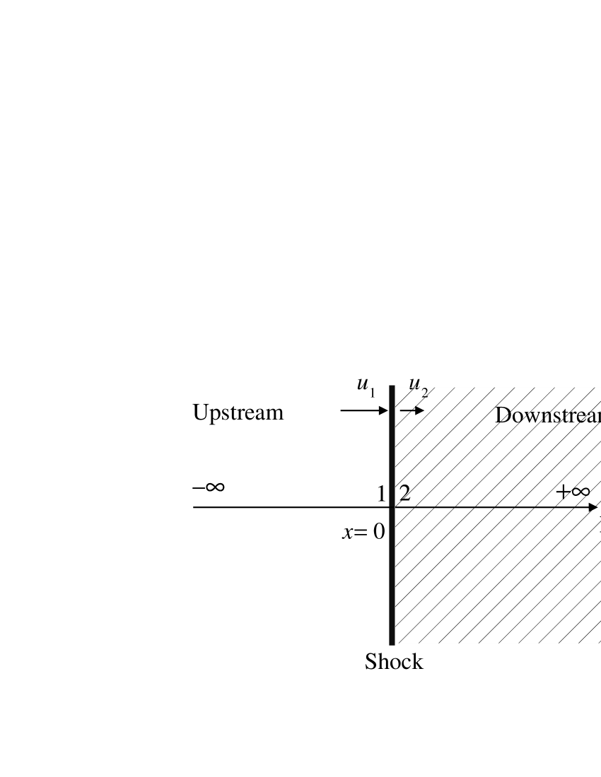
Figure 1: Schematic view of the shock region.

As a first step, we integrate Eq. 1 around $x=0$, from $x=0^{-}$ to $x=0^{+}$, denoted in fig. 1 as points “1” and “2” respectively, so that the following equation can be written:

$$\left[D\frac{\partial f}{\partial x}\right]_{2}-\left[D\frac{\partial f}{\partial x}\right]_{1}+\frac{1}{3}p\frac{df_{0}}{dp}(u_{2}-u_{1})+Q_{0}(p)=0,$$ (2)

where $u_{1}$ ($u_{2}$) is the fluid speed immediately upstream (downstream) of the shock and $f_{0}$ is the particle distribution function at the shock location. By requiring that the distribution function downstream is independent of the spatial coordinate (homogeneity), we obtain $\left[D\frac{\partial f}{\partial x}\right]_{2}=0$, so that the boundary condition at the shock can be rewritten as

$$\left[D\frac{\partial f}{\partial x}\right]_{1}=\frac{1}{3}p\frac{df_{0}}{dp}(u_{2}-u_{1})+Q_{0}(p).$$ (3)

We can now perform the integration of Eq. 1 from $x=-\infty$ to $x=0^{-}$ (point “1”), in order to take into account the boundary condition at upstream infinity. Using Eq. 3 we obtain

$$\frac{1}{3}p\frac{df_{0}}{dp}(u_{2}-u_{1})-u_{1}f_{0}+Q_{0}(p)+\int_{-\infty}^{0^{-}}dxf\frac{du}{dx}+$$

$$~{}~{}~{}~{}~{}\frac{1}{3}\int_{-\infty}^{0^{-}}dx\frac{du}{dx}p\frac{\partial f}{\partial p}=0.$$ (4)

We introduce the quantity $u_{p}$ defined as

$$u_{p}=u_{1}-\frac{1}{f_{0}}\int_{-\infty}^{0^{-}}dx\frac{du}{dx}f(x,p),$$ (5)

whose physical meaning is instrumental to understand the nonlinear reaction of particles. The function $u_{p}$ is the average fluid velocity experienced by particles with momentum $p$ while diffusing upstream away from the shock surface. In other words, the effect of the average is that, instead of a constant speed $u_{1}$ upstream, a particle with momentum $p$ experiences a spatially variable speed, due to the pressure of the accelerated particles. Since the diffusion coefficient is in general $p$-dependent, particles with different energies feel a different compression coefficient, higher at higher energies if, as expected, the diffusion coefficient is an increasing function of momentum (see (Blasi 2004) for further details on the meaning of the quantity $u_{p}$).

With the introduction of $u_{p}$, Eq. 4 becomes

$$\frac{1}{3}p\frac{df_{0}}{dp}(u_{2}-u_{p})-f_{0}\left[u_{p}+\frac{1}{3}p\frac{du_{p}}{dp}\right]+Q_{0}(p)=0,$$ (6)

where we used the fact that

$$p\frac{d}{dp}\int_{-\infty}^{0^{-}}dx\frac{du}{dx}f=p\left[\frac{df_{0}}{dp}(u_{1}-u_{p})-f_{0}\frac{du_{p}}{dp}\right].$$

The solution of Eq. 6 for a monochromatic injection at momentum $p_{inj}$ is

$$f_{0}(p)=$$

$$\int_{p_{0}}^{p}\frac{d{\bar{p}}}{{\bar{p}}}\frac{3Q_{0}({\bar{p}})}{u_{\bar{p}}-u_{2}}\exp\left\{-\int_{\bar{p}}^{p}\frac{dp^{\prime}}{p^{\prime}}\frac{3}{u_{p^{\prime}}-u_{2}}\left[u_{p^{\prime}}+\frac{1}{3}p^{\prime}\frac{du_{p^{\prime}}}{dp^{\prime}}\right]\right\}=$$

$$\frac{3R_{sub}}{R_{sub}-1}\frac{\eta n_{gas,1}}{4\pi p_{inj}^{3}}\times$$

$$\times\exp\left\{-\int_{p_{inj}}^{p}\frac{dp^{\prime}}{p^{\prime}}\frac{3}{u_{p^{\prime}}-u_{2}}\left[u_{p^{\prime}}+\frac{1}{3}p^{\prime}\frac{du_{p^{\prime}}}{dp^{\prime}}\right]\right\}.$$ (7)

Here we used $Q_{0}(p)=\frac{\eta n_{gas,1}u_{1}}{4\pi p_{inj}^{2}}\delta(p-p_{inj})$, with $n_{gas,1}$ the gas density immediately upstream ($x=0^{-}$) and $\eta$ the fraction of the particles crossing the shock which take part in the acceleration process.

Here we introduced the two quantities $R_{sub}=u_{1}/u_{2}$ and $R_{tot}=u_{0}/u_{2}$, which are respectively the compression factor at the gas subshock and the total compression factor between upstream infinity and downstream. For a modified shock, $R_{tot}$ can attain values much larger than $R_{sub}$ and more in general, much larger than $4$, which is the maximum value achievable for an ordinary strong non-relativistic shock. The increase of the total compression factor compared with the prediction for an ordinary shock is responsible for the peculiar flattening of the spectra of accelerated particles that represents a feature of nonlinear effects in shock acceleration. In terms of $R_{sub}$ and $R_{tot}$ the density immediately upstream is $n_{gas,1}=(\rho_{0}/m_{p})R_{tot}/R_{sub}$.

In Eq. 7 we can introduce a dimensionless quantity $U(p)=u_{p}/u_{0}$ so that

$$f_{0}^{inj}(p)=\left(\frac{3R_{sub}}{R_{tot}U(p)-1}\right)\frac{\eta n_{gas,1}}{4\pi p_{inj}^{3}}\times$$

$$\times\exp\left\{-\int_{p_{inj}}^{p}\frac{dp^{\prime}}{p^{\prime}}\frac{3R_{tot}U(p^{\prime})}{R_{tot}U(p^{\prime})-1}\right\}.$$ (8)

The nonlinearity of the problem reflects in the fact that $U(p)$ is in turn a function of $f_{0}$ as it is clear from the definition of $u_{p}$. In order to solve the problem we need to write the equations for the thermodynamics of the system including the gas, the cosmic rays accelerated from the thermal pool and the shock itself.

The velocity, density and thermodynamic properties of the fluid can be determined by the mass and momentum conservation equations, with the inclusion of the pressure of the accelerated particles. We write these equations between a point far upstream ($x=-\infty$), where the fluid velocity is $u_{0}$ and the density is $\rho_{0}=mn_{gas,0}$, and the point where the fluid velocity is $u_{p}$ (density $\rho_{p}$). The index $p$ denotes quantities measured at the point where the fluid velocity is $u_{p}$, namely at the point $x_{p}$ that can be reached only by particles with momentum $\geq p$ (this is clearly an approximation, but as shown in section 4 it provides a good agreement with other calculations where this approximation is not used).

The mass conservation implies:

$$\rho_{0}u_{0}=\rho_{p}u_{p}.$$ (9)

Conservation of momentum reads:

$$\rho_{0}u_{0}^{2}+P_{g,0}=\rho_{p}u_{p}^{2}+P_{g,p}+P_{CR,p},$$ (10)

where $P_{g,p}$ is the gas pressure at the point $x=x_{p}$ and $P_{CR,p}$ is the pressure of accelerated particles at the same point (we use the symbol $CR$ to mean cosmic rays, in the sense of accelerated particles). The mass and momentum escaping fluxes in the form of accelerated particles have reasonably been neglected. Note that at this point the equation for energy conservation has not been used.

Our basic assumption, similar to that used in (Eichler 1984), is that the diffusion is $p$-dependent and more specifically that the diffusion coefficient $D(p)$ is an increasing function of $p$. Therefore the typical distance that a particle with momentum $p$ travels away from the shock is approximately $\Delta x\sim D(p)/u_{p}$, larger for high energy particles than for lower energy particles. As a consequence, at each given point $x_{p}$ only particles with momentum larger than $p$ are able to affect appreciably the fluid. Strictly speaking the validity of the assumption depends on how strongly the diffusion coefficient depends on the momentum $p$ (see section 4).

Since only particles with momentum $\geq p$ can reach the point $x=x_{p}$, we can write

$$P_{CR,p}\simeq\frac{4\pi}{3}\int_{p}^{p_{max}}dpp^{3}v(p)f_{0}(p),$$ (11)

where $v(p)$ is the velocity of particles with momentum $p$, $p_{max}$ is the maximum momentum achievable in the specific situation under investigation.

From Eq. 10 we can see that there is a maximum distance, corresponding to the propagation of particles with momentum $p_{max}$ such that at larger distances the fluid is unaffected by the accelerated particles and $u_{p}=u_{0}$.

The equation for momentum conservation is:

$$\frac{dU}{dp}\left[1-\frac{1}{M_{0}^{2}}U^{-(\gamma_{g}+1)}\right]+\frac{1}{\rho_{0}u_{0}^{2}}\frac{dP_{CR}}{dp}=0.$$ (12)

Using the definition of $P_{CR}$ and multiplying by $p$, this equation becomes

$$p\frac{dU}{dp}\left[1-\frac{1}{M_{0}^{2}}U^{-(\gamma_{g}+1)}\right]=\frac{4\pi}{3\rho_{0}u_{0}^{2}}p^{4}v(p)f_{0}(p),$$ (13)

where $f_{0}$ is known once $U(p)$ is known. Eq. 13 is therefore an integral-differential nonlinear equation for $U(p)$. The solution of this equation also provides the spectrum of the accelerated particles.

The last missing piece is the connection between $R_{sub}$ and $R_{tot}$, the two compression factors appearing in Eq. 8. The compression factor at the gas shock around $x=0$ can be written in terms of the Mach number $M_{1}$ of the gas immediately upstream through the well known expression

$$R_{sub}=\frac{(\gamma_{g}+1)M_{1}^{2}}{(\gamma_{g}-1)M_{1}^{2}+2}.$$ (14)

On the other hand, if the upstream gas evolution is adiabatic, then the Mach number at $x=0^{-}$ can be written in terms of the Mach number of the fluid at upstream infinity $M_{0}$ as

$$M_{1}^{2}=M_{0}^{2}\left(\frac{u_{1}}{u_{0}}\right)^{\gamma_{g}+1}=M_{0}^{2}\left(\frac{R_{sub}}{R_{tot}}\right)^{\gamma_{g}+1},$$

so that from the expression for $R_{sub}$ we obtain

$$R_{tot}=M_{0}^{\frac{2}{\gamma_{g}+1}}\left[\frac{(\gamma_{g}+1)R_{sub}^{\gamma_{g}}-(\gamma_{g}-1)R_{sub}^{\gamma_{g}+1}}{2}\right]^{\frac{1}{\gamma_{g}+1}}.$$ (15)

Now that an expression between $R_{sub}$ and $R_{tot}$ has been found, Eq. 13 basically is an equation for $R_{sub}$, with the boundary condition that $U(p_{max})=1$. Finding the value of $R_{sub}$ (and the corresponding value for $R_{tot}$) such that $U(p_{max})=1$ also provides the whole function $U(p)$ and, through Eq. 8, the distribution function $f_{0}(p)$. If the reaction of the accelerated particles is small, the test particle solution is recovered.

3 The appearance of multiple solutions

In the problem described in the previous section there are several independent parameters. While the Mach number of the shock and the maximum momentum of the particles are fixed by the physical conditions in the environment, the injection momentum and the acceleration efficiency are free parameters. The procedure to be followed to determine the solution was defined in (Blasi 2002): the basic problem is to find the value of $R_{sub}$ (and therefore of $R_{tot}$) for which $U(p_{max})=1$. In Fig. 2 we plot $U(p_{max})$ as a function of $R_{tot}$, for $T_{0}=10^{5}K$, $p_{max}=10^{5}mc$ and $p_{inj}=10^{-2}mc$ in the left panel and $p_{inj}=10^{-3}mc$ in the right panel ($m$ here is the mass of protons). The parameter $\eta$ was taken $10^{-4}$ in the left panel and $10^{-3}$ in the right panel. The different curves refer to different choices of the Mach number at upstream infinity. The physical solutions are those corresponding to the intersection points with the horizontal line $U(p_{max})=1$, so that multiple solutions occur for those values of the parameters for which there is more than one intersection with $U(p_{max})=1$. These solutions are all physically acceptable, as far as the conservation of mass, momentum and energy are concerned.

Figure 2: Left panel: $U(p_{max})$ as a function of the total compression factor for $T_{0}=10^{5}$ K, $\eta=10^{-4}$, $p_{max}=10^{5}~{}mc$ and $p_{inj}=10^{-2}~{}mc$ for the Mach numbers indicated. Right panel: same as in left panel but for $\eta=10^{-3}$ and $p_{inj}=10^{-3}~{}mc$.

It can be seen from both panels in Fig. 2 that for low values of the Mach number, only one solution is found. This solution may be significantly far from the quasi-linear solution. Indeed, for $M_{0}=10$ the solution corresponds to $R_{tot}\sim 8$, instead of the usual $R_{tot}\sim 4$ solution expected in the linear regime. Lower values of the Mach number are required to fully recover the linear solution.

When the Mach number is increased, there is a threshold value for which three solutions appear, one of which is the quasi-linear solution. For very large values of the Mach number the solution becomes one again, and it coincides with the quasi-linear solution.

Figure 3: Left panel:$U(p_{max})$ as a function of the total compression factor for $T_{0}=10^{5}$ K, $p_{max}=10^{5}~{}mc$ and $p_{inj}=10^{-3}~{}mc$ at fixed Mach number $M_{0}=100$ for the efficiencies indicated. Right panel: same as in left panel but for $p_{inj}=10^{-2}~{}mc$.

In Fig. 3 we show the appearance of the multiple solutions for the case $T_{0}=10^{5}K$, $p_{max}=10^{5}mc$ and $p_{inj}=10^{-3}mc$ with Mach number $M_{0}=100$ ($p_{inj}=10^{-2}mc$ and $M_{0}=100$) in the left (right) panel. The curves here are obtained by changing the value of $\eta$. The same comments we made for Fig. 2 apply here as well: low values of $\eta$ correspond to weakly modified shocks, while for increasingly larger efficiencies multiple solutions appear. The solution becomes one again in the limit of large efficiencies, and it always corresponds to strongly modified shocks.

The problem of multiple solutions is not peculiar of the kinetic approaches to the non-linear theories of particle acceleration at shock waves. The same phenomenon was in fact found initially in two-fluid models (Drury & Völk 1980, 1981), where however no information on the spectrum of the accelerated particles and on the injection efficiency was available.

4 Comparison with an alternative approach

Multiple solutions were also found by Malkov (1997) and Malkov et al. (2000), in the context of a semi-analytical kinetic approach. Aside from the technical differencies between that method and the one proposed by Blasi (2002, 2004), the main difference is in the fact that the former requires the knowledge of the exact expression for the diffusion coefficient as a function of the momentum of the particles, while the latter only requires that such diffusion coefficient is an increasing function of the particle momentum. While the first approach may provide us with an exact solution to the problem, the second is in fact more practical, in the sense of providing an approximate solution even in those cases, the majority, in which no detailed information on the diffusion properties of the fluid is available. The solution provided in (Blasi 2002, 2004) is particularly accurate when the diffusion coefficient is Bohm-like, $D(p)=(1/3)r_{L}c$, expected in the case of saturated self-generation of waves in the vicinity of the shock surface (Lagage & Cesarsky 1983).

We will now discuss the quantitative comparison between the results of Malkov (1997) and those of Blasi (2002, 2004), by considering a single situation in which multiple solutions are predicted (in both approaches), and determining the spectra and compression factors in both methods. We start with briefly summarizing the approach of Malkov (1997). The following flow potential is introduced there:

$$\Psi=\int_{x}^{0}dx^{\prime}u(x^{\prime}),$$ (16)

which is used as a new independent spatial variable to replace $x$. Using the flow potential, it is possible to define an integral transformation of the flow profile as follows:

$$\hat{U}(p)=\frac{1}{u_{0}}\int^{-\infty}_{0^{+}}\exp\left[-\frac{q(p)}{3D(p)}\Psi\right]\frac{du}{dx}dx,$$ (17)

where $q(p)=-d\ln f_{0}/d\ln p$ is the spectral index of the particle distribution function and $D(p)$ is the diffusion coefficient, which is assumed to be independent of the position. An integral equation for $\hat{U}(p)$ can be derived by applying Eq. 17 to the $x$–derivative of the Euler equation (Malkov 1997; Malkov et al. 2000):

$$\hat{U}(p)=\frac{R_{sub}-1}{R_{tot}}+$$

$$\frac{\nu}{p_{inj}}\int_{p_{inj}}^{p_{max}}d\hat{p}\frac{\hat{p}}{\sqrt{\hat{p}^{2}+(mc)^{2}}}\left[1+\frac{q(p)D(\hat{p})}{q(\hat{p})D(p)}\right]^{-1}\times$$

$$\times\frac{\hat{U}(p_{inj})}{\hat{U}(\hat{p})}\exp\left[-\frac{3}{RR_{sub}}\int_{p_{inj}}^{\hat{p}}\frac{d\ln p^{\prime}}{\hat{U}(p^{\prime})}\right],$$ (18)

where $\nu$ is an injection parameter defined as

$$\nu=\frac{4\pi}{3}\frac{c}{\rho_{0}u_{0}^{2}}p_{inj}^{4}f_{0}(p_{inj}),$$ (19)

and related to the compression factor by the following equation (Malkov 1997):

$$\nu=p_{inj}(1-\frac{1}{R})\Bigg{\{}\int_{p_{inj}}^{p_{max}}dp\frac{p}{\sqrt{p^{2}+(mc)^{2}}}\frac{\hat{U}(p_{inj})}{\hat{U}(p)}\times$$

$$~{}~{}~{}~{}~{}\exp\left[-\frac{3}{R_{sub}R}\int_{p_{inj}}^{p}\frac{d\ln p^{\prime}}{\hat{U}(p^{\prime})}\right]\Bigg{\}}^{-1}.$$ (20)

Here $R=R_{tot}/R_{sub}$ is the compression factor in the shock precursor. Eqs. 15, 18 and 20 form a closed system that can be solved numerically.

Before showing the results it is worth noticing that the injection parameters $\eta$ and $\nu$ adopted in the two approaches are defined in two non equivalent ways. However, the relation between $\eta$ and $\nu$ can easily be found by using Eqs. 8 and 19 and can be written as:

$$\nu=\eta\left(\frac{p_{inj}c}{mu_{0}^{2}}\right)\frac{R_{tot}}{R_{sub}-1}.$$ (21)

One may notice that this relation contains the compression factors $R_{tot}$ and $R_{sub}$, which are what we are searching for. This fact implies that three solutions characterized by the same value of $\eta$ may correspond to three distinct values of $\nu$.

In order to compare the results of the two different approaches we consider a shock having Mach number $M_{0}=150$ and temperature at upstream infinity $T_{0}=10^{4}K$. We set the value of the injection and maximum momenta equal to $10^{-3}mc$ and $10^{5}mc$ respectively and we adopt an efficiency $\eta=10^{-4}$. Using the approach proposed by Blasi (2002), we find three solutions, characterized by the values of the compression factor $R\sim 15.3,3.94,1.05$. The last solution is the quasi-linear one, in which the precursor is very weak. We adopt now these three values for the precursor compression factor to solve the system of equations given by Eq. 15, 18, and 20) for different choices of the diffusion coefficient.

In Fig. 4 we plot the velocity profiles for the three solutions, as derived with the method of Blasi (2002, 2004) and detailed above (solid line). In the figure $U(p)=u_{p}/u_{0}$ with $u_{p}$ defined through Eq. 5 for the method of Blasi (2002, 2004). It is easy to show that $U(p)$ is related to the $\hat{U}(p)$ through the relation $\hat{U}(p)+1/R_{t}ot=U(p)$. The dotted and dashed lines are the results obtained with the calculation of Malkov (1997) with a Bohm and Kolmogorov diffusion respectively. For Bohm diffusion the two approaches give very similar results. For Kolmogorov diffusion the differencies are larger, as expected.

Figure 4: Velocity profile upstream of the shock as derived in this paper (solid line) and with the approach of Malkov (1997) with a Bohm diffusion (dotted line) and for a Kolmogorov diffusion (dashed line).

In Fig. 5 we plot the spectra of the accelerated particles, as obtained in this paper (solid line) and for a Bohm (dotted line) and Kolmogorov (dashed line) diffusion coefficient, as derived by carrying out the calculation of Malkov (1997).

Figure 5: Spectrum of the accelerated particles as derived in this paper (solid line) and with the approach of Malkov (1997) with a Bohm diffusion (dotted line) and for a Kolmogorov diffusion (dashed line).

We recall that from the theoretical point of view the Bohm diffusion is in fact what should be expected in the proximity of a shock if the turbulence necessary for the acceleration is strong and generated by the same cosmic rays that are being accelerated (Lagage & Cesarsky 1983). In this perspective, we look at the results illustrated in this section as very encouraging in using the approach presented in Blasi (2002, 2004), since it is simple and at the same time accurate in reproducing the major physical aspects of particle acceleration at cosmic ray modified shocks.

5 A recipe for injection from the thermal pool

The presence of multiple solutions is typical of many non-linear problems and should not be surprising from the mathematical point of view. In terms of physical understanding however, multiple solutions may be disturbing. The typical situation that takes place in nature when multiple solutions appear in the description of other non linear systems is that (at least) one of the solutions is unstable and the system falls in a stable solution when perturbed. The stable solutions are the only ones that are physically meaningful. Some attempts to investigate the stability of cosmic ray modified shock waves have been made by Mond & Drury (1998) and Toptygin (1999), but all of them refer to the two-fluid models. A step forward is being carried out by Blasi & Vietri (in preparation) in the context of kinetic models.

In addition to the stability, another issue that enters the physical description of our problem is the identification of possible processes that determine some type of backreaction on the system. It may be expected that when some types of processes of self-regulation are included, the phenomenon of multiple solutions is reduced. In this section we investigate the type of reaction that takes place when a self-consistent, though simple, recipe for the injection of particles from the thermal pool is adopted. This recipe is similar to that proposed by Kang, Jones & Gieseler (2002) in terms of the underlying physical interpretation of the injection, but probably simpler in its implementation.

For non-relativistic shocks, the distribution of particles downstream is quasi-isotropic, so that the flux of particles crossing the shock surface from downstream to upstream can be written as

$$\Phi=-2\pi~{}\int_{p_{min}}^{\infty}dp\int_{-1}^{-u_{d}/v(p)}d\mu\frac{f_{th}(p)}{4\pi}4\pi p^{2}\left[u_{d}+v(p)\mu\right],$$ (22)

where $v(p)$ is the velocity of particles with momentum $p$ and $u_{d}$ is the shock speed in the frame comoving with the downstream fluid. The term $u_{d}+v(p)\mu$ is the component along the direction perpendicular to the shock surface of the velocity of particles with momentum $p$ moving in the direction $\mu$. It follows that the flux of particles moving tangent to the shock surface (namely with $\mu=-u_{d}/v(p)$) is zero. We recall that, having in mind collisionless shocks, the typical thickness of the shock, $\lambda$, is the collision length associated with the magnetic interactions that give rise to the formation of the discontinuity. Useless to say that these interactions are all but well known, and at present the best we can do is to attempt a phenomenological approach to take them into account, without having to deal with their detailed physical understanding. It is however worth recalling that many attempts have been made to tackle the problem of injection at a more fundamental level (Malkov 1998; Malkov & Völk 1995; Malkov & Völk 1998). Here, we consider the reasonable situation in which $\lambda\propto r_{L}^{th}$, where $r_{L}^{th}\propto p_{th}$ is the Larmor radius of the particles in the downstream fluid that carry most of the thermal energy, namely those with momentum $1.5~{}p_{th}$ ($p_{th}=(2mk_{B}T_{2})^{1/2}$ here is the momentum of the particles in the thermal peak of the maxwellian distribution in the downstream plasma, having temperature $T_{2}$). We stress here the important point that the temperature of the downstream gas (and therefore $p_{th}$) is determined by the shock strength, which in the presence of accelerated particles, is affected by the pressure of the non-thermal component. In particular, the higher the efficiency of the shock as a particle accelerator, the weaker its efficiency in terms of heating of the background plasma (see section 8).

For collisionless shocks, it is not clear whether the downstream plasma can actually be thermalized and the distribution function be a maxwellian. On the other hand, it is generally assumed that this is the case, so that in the following we consider the case in which the bulk of the background plasma is thermal and has a maxwellian spectrum at temperature $T$ given by the generalized Rankine-Hugoniot relations in the presence of accelerated particles (see section 2). For modified shocks, the points discussed above apply to the so-called subshock, where the injection of particles from the thermal pool is expected to take place. We recall that for strongly modified shocks the subshock is weak, and rather inefficient in the heating of the background plasma.

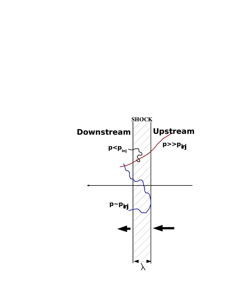
Figure 6: Graphic illustration of the structure of a collisionless shock and of the basic idea underlying our injection recipe.

From Eq. 22 we get:

$$\Phi=\frac{1}{4}\int_{p_{min}}^{\infty}dp4\pi p^{2}f_{th}(p)\frac{(v(p)-u_{d})^{2}}{v(p)},$$ (23)

where we assumed that the temperature downstream implies non-relativistic motion of the quasi-thermal particles ($p\approx mv(p)$). In Eq. 23 we write the minimum momentum in terms of a parameter $\alpha$, such that $\lambda=\alpha r_{L}^{th}$. With this formalism, the particles that can cross the shock surface are those that satisfy the condition:

$$p>p_{min}=1.5~{}\alpha~{}p_{th}.$$ (24)

The parameter $\alpha$ defines the thickness of the shock in units of the gyration radius of the bulk of the thermal particles. Our recipe for injection is pictorially illustrated in Fig. 6: thermal particles have a pathlength smaller than the shock thickness and cannot cross the shock surface, being advected downstream before the crossing occurs. Only particles with momentum sufficiently larger than the thermal momentum of the downstream particles can actually return upstream and be accelerated.

In the following we will neglect the fluid speed $u_{d}$ compared with $v(p)$, which is a good approximation if the injected particles are sufficiently more energetic than the thermal particles. This is done only to make the interpretation of the result simpler, but there is no technical difficulty in keeping the dependence of the results on $u_{d}$.

We introduce an effective injection momentum $p_{inj}=\xi p_{th}$ defined by the equation:

$$\Phi=\int_{\xi p_{th}}^{\infty}dp4\pi p^{2}f_{th}(p)v(p),$$ (25)

which in terms of dimensionless quantities, with $f_{th}(p)=e^{-(p/p_{th})^{2}}$ reads:

$$\int_{1.5\alpha}^{\infty}dxx^{3}e^{-x^{2}}=4\int_{\xi}^{\infty}dxx^{3}e^{-x^{2}}.$$ (26)

It is easy to show that $\xi\approx 2$ for $\alpha=1$ (half a Larmor rotation of the particles with momentum $1.5p_{th}$ inside the thickness of the shock) and $\xi\approx 3.25$ for $\alpha=2$ (one full Larmor rotation of the particles with momentum $1.5p_{th}$ inside the thickness of the shock. The fraction of particles at momentum $\xi$ times larger than the thermal one is $\sim 5\%$ for $\xi=2$ and $\sim 10^{-4}$ for $\xi=3.25$. The actual values of $\xi$ are expected to be somewhat higher if the effect of advection with the downstream fluid is not neglected. The sharp decrease in the fraction of leaking particles that may take part in the acceleration process is due to the exponential behaviour of the maxwellian at large momenta. Although the fraction of particles in the maxwellian that get accelerated only depends on the parameter $\xi$ which in turn is expected to keep the information about the microscopic structure of the shock, the absolute number of and energy carried by these particles depend on the temperature of the downstream gas, which is an output of our calculation. This simple argument serves as an explanation of the physical reason why there is a nonlinear reaction on the system due to injection. If the parameter $\xi$ is assumed to be determined by the microphysics of the shock, and if we adopt our simple recipe to describe such microphysics, then the shock thickness is easily estimated once the temperature of the downstream gas is known, and the latter can be calculated from the modified Rankine-Hugoniot relations. The parameter $\eta$ in Eq. 8 is no longer a free parameter, being related in a unique way to the parameter $\xi$ and to the physical conditions at the subshock. The condition that fixes $\eta$ is that the total number of particles in the non-thermal spectrum equals the number of particles in the maxwellian at momenta larger than $p_{inj}$. Due to the very strong dependence of the spectrum on the momentum for both the maxwellian and the power law at low momenta, the condition described above is very close to require the continuity of the distribution function, namely that $f_{th}(p_{inj})=f_{0}(p_{inj})$. In the following we adopt this condition for the calculations. This can be shown to imply the following expression for $\eta$:

$$\eta=\frac{4}{3\pi^{1/2}}(R_{sub}-1)\xi^{3}e^{-\xi^{2}}.$$ (27)

We recall that the compression factor at the subshock, $R_{sub}$, approaches unity when the shock becomes cosmic ray dominated. This makes evident how the backreaction discussed above works: when the shock becomes increasingly more modified, the efficiency $\eta$ tends to decrease, limiting the amount of energy that can be channelled in the non-thermal component. Although the recipe provided here is certainly far from representing the complexity of the reality of injection of particles from the thermal pool, it may be considered as a useful attempt to include the main physical aspects of this phenomenon.

6 Self-consistent injection and multiple solutions

In this section we describe the role played by the injection recipe discussed above for the appearance of multiple solutions. It can be expected that the phenomenon is somewhat reduced because, as discussed in the previous section, the injection provides an efficient backreaction mechanism on the shock as a particle accelerator. Indeed we find that the appearance of multiple solutions is drastically reduced, and that the phenomenon still exists only in regions of the parameter space which are very narrow and of limited physical interest. In the quantitative calculations we use the value $\xi=3.5$ for the injection parameter, as suggested by the simple estimate in Section 5 and as suggested also in the numerical work of Kang & Jones (1995). The dependence of the effect on the value of $\xi$ is discussed below. In Fig. 7 we illustrate the dramatic change in the physical picture by plotting $U(p_{max})$ as a function of $R_{tot}$ for $\xi=3.5$ and adopting the same values for the parameters as those used in obtaining Fig. 2. The efficiency $\eta$ is now calculated according with the recipe described in the previous section. It can be seen very clearly that when the Mach number of the shock is changed, there is a single solution (compare with Fig. 2 where multiple solutions where found for the same values of the parameters, but without thermal leakage).

Figure 7: $U(p_{max}$ as a function of the total compression factor for $T_{0}=10^{5}$ K, $p_{max}=10^{5}~{}mc$ and $\xi=3$ for the Mach numbers indicated.

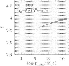
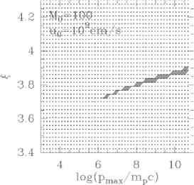
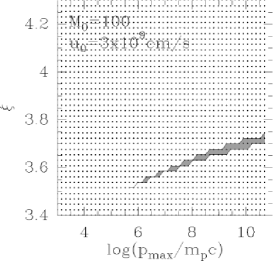
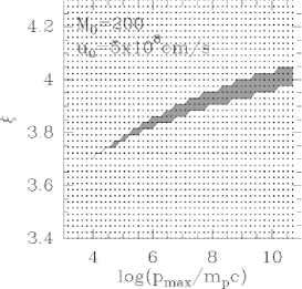
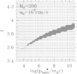
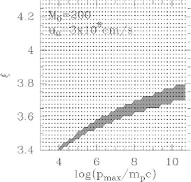
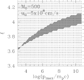
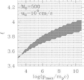
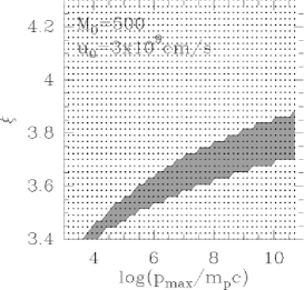
Figure 8: Parameter space for multiple solutions. The dark regions illustrate the regions of parameters for which multiple solutions are still present.

The appearance of multiple solutions can be investigated in the whole parameter space, in order to define the regions where the phenomenon appears, when it does. In Fig. 8 we highlight the regions where there are multiple solutions (dark regions) in a plane $\xi-\log(p_{max})$, for different values of the Mach number of the shock. In most cases the dark regions are very narrow and cover a region of values of $\xi$ which is rather high (small efficiency). In Fig. 9 we plot the value of $R_{tot}$ as a function of $\xi$ for $M_{0}=200$, $u_{0}=5\times 10^{8}\rm cm~{}s^{-1}$ and $p_{max}=10^{3},10^{4},~{}10^{5},~{}10^{7}~{}mc$ from left to right. The line is continuous when there are no multiple solutions and dashed when multiple solutions appear. The dashed regions are, as stressed above, rather narrow. For instance, for $p_{max}=10^{4}mc$ there are multiple solutions only for $3.67\leq\xi\leq 3.7$. Any small perturbation of the system that changes the values of $\xi$ at the percent level implies that the system shifts to one of the single solutions if it is sitting in the intermediate solution before the perturbation. The sharp transition between the strongly modified solution and the quasi-linear solution when $\xi$ is increased suggests that the intermediate solution may be unstable, though a formal demonstration cannot be provided here. In order to make sure that this is the case, a careful analysis of the stability is required, and will be presented in a forthcoming publication (Blasi & Vietri, in preparation). On the other hand, a previous study, carried out in the context of the two-fluid models, showed that when multiple solutions are present, the solution with intermediate efficiency is in fact unstable to corrugations of the shock surface (Mond and Drury 1998).

Figure 9: Dependence of $R_{tot}$ as a function of $\xi$ for $M_{0}=200$, $u_{0}=5\times 10^{8}\rm cm~{}s^{-1}$ and $p_{max}=10^{3},10^{4},~{}10^{5},~{}10^{7}~{}mc$ from left to right. The sharpness of the transition suggests that the small perturbations of the parameters make the solution fall on one of the two sides.

7 Escaping flux of accelerated particles

It is rather remarkable that the kinetic model of Blasi (2002, 2004) does not require explicitely the use of the equation for energy flux conservation. However, once the solution of the kinetic problem has been found, the equation for conservation of the energy flux provides very useful information, as we show below. The equation can be written in the following form:

$$\frac{1}{2}\rho_{2}u_{2}^{3}+\frac{\gamma_{g}}{\gamma_{g}-1}P_{g,2}u_{2}+\frac{\gamma_{c}}{\gamma_{c}-1}P_{c,2}u_{2}=$$

$$~{}~{}~{}~{}~{}~{}~{}~{}~{}~{}\frac{1}{2}\rho_{0}u_{0}^{3}+\frac{\gamma_{g}}{\gamma_{g}-1}P_{g,0}u_{0}-F_{E},$$ (28)

where $F_{E}$ is the flux of particles escaping at the maximum momentum from the upstream section of the fluid (Berezhko & Ellison, 1999). Notice that this term is usually neglected in the linear approach to particle acceleration at shock waves because the spectra are steep enough that, in most cases, we can neglect the flux of particles leaving the system at the maximum momentum. The fact that particles leave the system make the upstream fluid behave as a radiative fluid, and makes it more compressible. This is a crucial consequence of particle acceleration at modified shocks, and is shown here to be a natural consequence of energy conservation.

Figure 10: Escaping flux ($F_{E}^{\prime}$), advected flux ($F_{adv}^{\prime}$) and the sum of the two ($F_{tot}^{\prime}$) normalized to the incoming flux $(1/2)\rho_{0}u_{0}^{3}$, as functions of the Mach number at upstream infinity $M_{0}$. Left panel: $u_{0}=5\times 10^{8}~{}\rm cm~{}s^{-1}$, $p_{max}=10^{6}~{}mc$ and $\xi=3.5$. Right Panel: $u_{0}=5\times 10^{8}~{}\rm cm~{}s^{-1}$, $p_{max}=10^{2}~{}mc$ and $\xi=3.5$.

In Eq. 28 we can divide all terms by $(1/2)\rho_{0}u_{0}^{3}$ and calculate the normalized escaping flux:

$$F_{E}^{\prime}=1-\frac{1}{R_{tot}^{2}}+\frac{2}{M_{0}^{2}(\gamma_{g}-1)}-\frac{2}{R_{tot}}\frac{\gamma_{g}}{\gamma_{g}-1}\frac{P_{g,2}}{\rho_{0}u_{0}^{2}}$$

$$~{}~{}~{}~{}~{}-\frac{2}{R_{tot}}\frac{\gamma_{c}}{\gamma_{c}-1}\frac{P_{c,2}}{\rho_{0}u_{0}^{2}}.$$ (29)

From momentum conservation at the subshock we also have:

$$\frac{P_{c,2}}{\rho_{0}u_{0}^{2}}=\frac{R_{sub}}{R_{tot}}-\frac{1}{R_{tot}}+\frac{1}{\gamma_{g}M_{0}^{2}}\left(\frac{R_{sub}}{R_{tot}}\right)^{-\gamma_{g}},$$ (30)

so that the escaping flux only depends upon the environment parameters (for instance the Mach number at upstream infinity) and the compression parameter $R_{sub}$ which is part of the solution. Note also that the adiabatic index for cosmic rays, $\gamma_{c}$, is here calculated self-consistently as:

$$\gamma_{c}=1+\frac{P_{c}}{E_{c}}=1+\frac{\frac{1}{3}\int_{p_{inj}}^{p_{max}}dp4\pi p^{3}v(p)f_{0}(p)}{\int_{p_{inj}}^{p_{max}}dp4\pi p^{2}f_{0}(p)\epsilon(p)},$$ (31)

where $E_{c}$ is the energy density in the form of accelerated particles and $\epsilon(p)$ is the kinetic energy of a particle with momentum $p$. It can be easily seen that $\gamma_{c}\to 4/3$ when the energy budget is dominated by the particles with $p\sim p_{max}$ (namely for strongly modified shocks) and $\gamma_{c}\to 5/3$ for weakly modified shocks. In Eq. 29 the term $F_{adv}^{\prime}=\frac{2}{R_{tot}}\frac{\gamma_{c}}{\gamma_{c}-1}\frac{P_{c,2}}{\rho_{0}u_{0}^{2}}$ is clearly the fraction of flux which is advected downstream with the fluid.

In Fig. 10 we plot the escaping flux ($F_{E}^{\prime}$), the advected flux ($F_{adv}^{\prime}$) and the sum of the two ($F_{tot}^{\prime}$) normalized to the incoming flux $(1/2)\rho_{0}u_{0}^{3}$, as functions of the Mach number at upstream infinity $M_{0}$. Here we used $u_{0}=5\times 10^{8}~{}\rm cm~{}s^{-1}$, and $\xi=3.5$, while the maximum momentum has been chosen as $p_{max}=10^{6}~{}mc$ in the left panel and $p_{max}=10^{2}~{}mc$ in the right panel. Several comments are in order:

• At low Mach numbers the escaping flux is inessential, as one would expect for a weakly modified shock. We recall that the escaping flux is due to the particles with momentum $p_{max}$ leaving the system from upstream infinity. For a weakly modified shock at low Mach number the spectrum is steeper than $E^{-2}$, so that the energy carried by the highest energy particles is a small fraction of the total.

• At large Mach numbers the shock becomes increasingly more cosmic ray dominated, and for the cases at hand the total efficiency gets very close to unity, meaning that the shock behaves as an extremely efficient accelerator. At Mach numbers around 4 on the other hand the total efficiency is around $20\%$ for $p_{max}=10^{6}~{}mc$ and $\sim 10\%$ for $p_{max}=10^{2}~{}mc$, dropping fast below Mach number 4. Clearly the efficiency would be higher in this region for lower values of the parameter $\xi$.

• Despite the fact that the total efficiency of the shock as a particle accelerator is close to unity at large Mach numbers, the fraction of the incoming energy which is actually advected toward downstream infinity is only $\sim 20\%$ at $M_{0}\approx 100$ for $p_{max}=10^{6}~{}mc$. Most of the enegy flux in this case is in fact in the form of energy escaping from upstream infinity at the highest momentum $p_{max}$. For $p_{max}=10^{2}~{}mc$ the normalized advected flux roughly saturates at $\sim 40\%$ and is comparable with the escape flux at the same Mach number. For a distant observer these escaping particles would have a spectrum close to a delta function around $p_{max}$.

8 Shock heating in the presence of efficient particle acceleration

Energy conservation has the natural consequence that a smaller fraction of the kinetic energy of the fluid is converted into thermal energy of the downstream plasma in cosmic ray modified shocks, compared with the case of ordinary shocks. The reduction of the heating at nonlinear shock waves is fully confirmed by our calculation in the context of the injection recipe introduced in section 5. In Fig. 11 we plot the temperature jump between downstream infinity (at temperature $T_{2}$) and upstream infinity (at temperature $T_{0}$). The thick solid line is the jump as predicted by the standard Rankine-Hugoniot relations without cosmic rays. The other lines represent the temperature jump at cosmic ray modified shocks with $p_{max}/mc=10^{3}$ (thin solid line), $p_{max}/mc=10^{5}$ (dashed line), $p_{max}/mc=10^{7}$ (dotted line) and $p_{max}/mc=5\times 10^{10}$ (dash-dotted line).

Figure 11: Temperature jump $T_{2}/T_{0}$ for $p_{max}/mc=10^{3}$ (thin solid line), $p_{max}/mc=10^{5}$ (dashed line), $p_{max}/mc=10^{7}$ (dotted line) and $p_{max}/mc=5\times 10^{10}$ (dash-dotted line). The thick solid line shows the jump for ordinary shocks.

Such a drastic reduction of the downstream temperature is expected to reflect directly in the thermal emission of the downstream gas in those environments in which collisions are relevant. Note that for strongly modified shocks the compression factor between upstream infinity and downstream are much larger than for ordinary shocks, so that the downstream turns out to be denser but colder than in the linear case. The missing energy ends up in the form of accelerated particles.

The effect of suppression of the heating in cosmic ray modified shocks also appears in the spectra of the particles (thermal plus non-thermal) in the shock vicinity. In Fig. 12 we show these spectra (including the maxwellian thermal bump) for $u_{0}=5\times 10^{8}~{}\rm cm~{}s^{-1}$, $\xi=3.5$ and $p_{max}/mc=10^{5}$.

Figure 12: Particle Spectra (thermal plus non-thermal) for $M_{0}=10$ (solid line), $M_{0}=50$ (dashed line) and $M_{0}=100$ (dotted line). The vertical dashed line represents the position of the thermal peak for ordinary shocks (it is almost independent of the Mach number for large Mach numbers).

The vertical dashed line shows the position of the thermal peak as expected in the absence of accelerated particles. In fact this position should depend on the Mach number, but the dependence is very weak for large Mach numbers. The positions of the thermal peaks clearly show the effect of cooler downstream gases for modified shocks. At the same time, the effect is accompanied by increasingly more modified spectra of accelerated particles, with most of the energy pushed toward the highest momenta.

9 Conclusions

The efficiency of the first order Fermi acceleration at shock fronts depends in a crucial way upon details of the mechanism that determines the injection of a small fraction of the particles from the thermal pool to the acceleration box. In reality the processes of formation of a collisionless shock wave, of plasma heating and particle acceleration are expected to be all parts of the same problem, though on different spatial scales. We hide our lack of knowledge of the microphysics of the shock structure in a simple recipe for injection, in which the particles that take part in the acceleration process are those that have momentum larger by a factor $\xi$ than the momentum of the thermal particles in the downstream fluid. This is motivated by the fact that for collisionless shocks the thickness of the shock surface is determined by the gyromotion of the bulk of the thermal particles. We estimated that $\xi\sim 2-4$. This recipe implies that the fraction of particles that get accelerated is rather small ($0.01-10^{-5}$).

We implemented this recipe in a calculation of the non-linear reaction of cosmic rays on the shock structure proposed by Blasi (2002, 2004). Similarly to other models, also this approach shows the appearance of multiple solutions, for a wide choice of the parameters of the problem. When the simple model of particle injection is used, this phenomenon is drastically reduced: the multiple solutions disappear for most of the parameter space, and when they appear they look as narrow strips in the parameter space, at the boundary between unmodified and modified shocks. We argued that this result suggests that the narrow regions may signal the transition between two stable solutions, although this needs further confirmation through detailed analyses of the stability of the solutions. This interpretation seems to be supported in part by the calculations of Mond & Drury (1998), that showed that when three solutions are present, the intermediate one is indeed unstable for small corrugations of the shock front. This calculations was however performed in the context of a two-fluid model, while an investigation of the stability for kinetic models is still lacking.

We find that the phenomenology of the particle acceleration at modified shocks is characterized by three main features:

• The modification of the shock increases with the Mach number of the fluid. For low Mach numbers the quasi-linear solution is recovered, but departures from it are evident already at relatively low Mach numbers. The modification of the spectra manifests itself with a hardening at high momenta and a softening at low momenta. The $p^{4}f_{0}(p)$ shows a characteristic dip at intermediate momenta, typically around $p/mc\sim 1-100$ (for very large values of $p_{max}$, the dip can be found at even larger momenta, which is of interest for the acceleration of ultra-high energy cosmic rays).

• The total efficiency for particle acceleration saturates at large Mach numbers at a number of order unity. However, as shown in Fig. 10, the largest fraction of the energy is not advected downstream but rather escapes from upstream infinity at the maximum momentum. This effect was also discussed in the context of the simple model by Berezhko & Ellison (1999).

• The high efficiency for particle acceleration reflects in a reduced ability of cosmic ray modified shocks in the heating of the background plasma. This effect is at the very basis of the backreaction introduced by the injection recipe on the acceleration process, and determines the saturation of the total efficiency for large Mach numbers. The heating suppression is shown in Fig. 11 and in Fig. 12.

References

- [1] Axford, W.I., Leer, E., and McKenzie, J.F., 1982, A&A 111, 317
- [2] Bell, A.R., 1978, MNRAS 182, 443
- [3] Bell, A.R., 1987, MNRAS 225, 615
- [4] Bell, A.R., 2004, MNRAS, 353, 550
- [5] Berezhko, E.G., 1996, Astropart. Phys. 5, 367
- [6] Berezhko, E.G., and Ellison, D.C., 1999, ApJ 526, 385
- [7] Berezhko, E.G. and Krimsky, G.F., 1988, Soviet. Phys.-Uspekhi 12, 155
- [8] Berezhko, E.G., Ksenofontov, L.T., and Yelshin, V.K., 1995, Nucl. Phys. B (Proc. Suppl.) 39A, 171
- [9] Berezhko, E.G., Yelshin, V.K., and Ksenofontov, L.T., 1994, Astropart. Phys. 2, 215
- [10] Blandford, R.D., 1980, Astrophys. J. 238, 410
- [11] Blandford, R.D. and Eichler, D., 1987, Phys. Rep. 154, 1
- [12] Blandford, R.D. and Ostriker, J.P., 1978, ApJ Lett. 221, 29
- [13] Blasi, P., 2002, Astropart. Phys. 16, 429
- [14] Blasi, P., 2004, Astropart. Phys. 21, 45
- [15] Drury, L .O’C., 1983, Rep. Prog. Phys. 46, 973
- [16] Drury, L.O’C, Axford, W.I. and Summers, D., 1982, MNRAS 198, 833
- [17] Drury, L.O’C and Völk, H.J., 1980, Proc. IAU Symp. 94, 363
- [18] Drury, L.O’C and Völk, H.J., 1981, ApJ 248, 344
- [19] Duffy, P., Drury, L.O’C. and Völk, H.J., 1994, A&A 291, 613
- [20] Eichler, D., 1984, ApJ 277, 429
- [21] Eichler, D, 1985, ApJ 294, 40
- [22] Ellison, D.C., Baring, M.G., and Jones, F.C., 1995, ApJ 453, 873
- [23] Ellison, D.C., Baring, M.G., and Jones, F.C., 1996, ApJ 473, 1029
- [24] Ellison, D., and Eichler, D., 1984, ApJ 286, 691
- [25] Ellison, D.C., and Eichler, E., 1985, Phys. Rev. Lett. 55, 2735
- [26] Ellison, D.C., Möbius, E., and Paschmann, G., 1990, ApJ 352, 376
- [27] Gieseler, U.D.J., Jones, T.W., and Kang, H., 2000, A&A 364, 911
- [28] Jones, F.C. and Ellison, D.C., 1991, Space Sci. Rev. 58, 259
- [29] Lagage, P. O., and Cesarsky, C. J., 1983, A&A, 118, 223
- [30] Kang, H. and Jones, T. W., 1995, ApJ 447, 944
- [31] Kang, H., and Jones, T.W., 1997, ApJ 476, 875
- [32] Kang, H., and Jones, T.W., 2005, ApJ 620, 44
- [33] Kang, H., Jones, T.W., and Gieseler, U.D.J., 2002, ApJ 579, 337
- [34] Lucek, S.G. and Bell, A.R., 2000, Astrop. & Space Sc. 272, 255
- [35] Lucek, S.G. and Bell, A.R., 2000a, MNRAS 314, 65
- [36] Bell, A.R., and Lucek, S.G., 2001, MNRAS 321, 433.
- [37] Malkov, M.A., 1997, ApJ 485, 638
- [38] Malkov, M.A., 1998, Phys. Rev. E 58, 4911
- [39] Malkov, M.A., Diamond P.H., and Völk, H.J., 2000, ApJ Lett. 533, 171
- [40] Malkov, M.A., and Drury, L.O’C., 2001, Rep. Prog. Phys. 64, 429
- [41] Malkov, M. A., and Völk, H. J., 1995, A&A 300, 605
- [42] Malkov, M. A., and Völk, H. J., 1998, Adv. Sp. Res 21, 551
- [43] Mond, M. and O’C. Drury, L., 1998, A&A 332, 385
- [44] Ptuskin, V.S. and Zirakashvili, V.N., 2003, A&A 403, 1
- [45] Ptuskin, V.S. and Zirakashvili, V.N., 2003a, preprint astro-ph/0306226
- [46] Toptygin, I. N., 1999, Astronomy Lett. 25, 34