Spitzer Observations of CO₂ Ice Towards Field Stars in the Taurus Molecular Cloud

Abstract

We present the first Spitzer Infrared Spectrograph observations of the 15.2 $\micron$ bending mode of CO₂ ice towards field stars behind a quiescent dark cloud. CO₂ ice is detected towards 2 field stars (Elias 16, Elias 3) and a single protostar (HL Tau) with an abundance of $\sim 15-20\%$ relative to water ice. CO₂ ice is not detected towards the source with lowest extinction in our sample, Tamura 17 (A_V = 3.9^m). A comparison of the Elias 16 spectrum with laboratory data demonstrates that the majority of CO₂ ice is embedded in a polar H₂O-rich ice component, with $\sim$15% of CO₂ residing in an apolar H₂O-poor mantle. This is the first detection of apolar CO₂ towards a field star. We find that the CO₂ extinction threshold is A${}_{V}=4^{m}\pm 1^{m}$, comparable to the threshold for water ice, but significantly less than the threshold for CO ice, the likely precursor of CO₂. Our results confirm CO₂ ice forms in tandem with H₂O ice along quiescent lines of sight. This argues for CO₂ ice formation via a mechanism similar to that responsible for H₂O ice formation, viz. simple catalytic reactions on grain surfaces.

1 Introduction

Observations by the Infrared Space Observatory (ISO) demonstrated that CO₂ ice is a ubiquitous component of the interstellar medium (ISM), with typical abundance of $\sim$15 – 25% relative to H₂O, the dominant ice component (Gerakines et al., 1999; Nummelin et al., 2001). However, the origin of this common grain mantle constituent remains uncertain. Gas-phase production, with subsequent freeze-out, is believed incapable of reproducing the observed abundance. In the laboratory CO₂ forms quite readily via ultraviolet (UV) photolysis or ion bombardment of astrophysical ice mixtures; along with the thermal processing of ices, these mechanisms have been suggested as possible formation routes (d’Hendecourt et al. 1986; Sandford et al. 1988; Palumbo et al. 1998). Even if UV photons and cosmic rays are not present with sufficient fluxes, an alternative mechanism is grain surface chemistry (Roser et al. 2001; Frost, Sharkey, & Smith 1991, and references therein). Observations of grain mantles indicate that there is competition between hydrogenation and oxidation of atoms on grain surfaces (van Dishoeck, 2004, and references therein). Nowhere is this more clear than for carbon-bearing molecules. CO₂ ice is less volatile than CO (Sandford & Allamandola, 1990) and its formation locks carbon in saturated form on grains, stopping any subsequent hydrogenation towards more complex molecules on grains or in the gas. Thus, an understanding of the formation mechanisms of CO₂ ice is needed in order to understand the limits of grain surface chemistry in producing more complex organics.

One way to constrain the origin of CO₂ ice in the ISM is to use bright field stars located behind molecular cloud material as candles that probe material remote from embedded sources, where, at suitably high extinction, ices are unlikely to be exposed to significant UV radiation or heating. ISO detected the CO₂ 4.27 $\mu$m $\nu_{3}$ stretching mode towards only two K giants, Elias 13 and 16 (Whittet et al., 1998; Nummelin et al., 2001). However, the detection of CO₂ ice towards any field star demonstrated that radiative processing of ices is unlikely to be responsible for the CO₂ ice production in quiescent material (Whittet et al., 1998).

In this paper we report, and discuss the implications of, the observation of the $\nu_{2}$ bending mode of CO₂ ice at 15.2 $\mu$m towards 3 field stars and 1 protostar in the Taurus molecular cloud using NASA’s Spitzer Space Telescope.

2 Observations and Results

Observations of each source (see Table 1) were obtained in 2004 using the Spitzer Infrared Spectrograph, hereafter IRS (Houck et al., 2004). Each object was observed in staring mode in the short-wavelength high-resolution mode spectrograph (Short-Hi;SH) which has coverage from 10 to 19 $\mu$m with $\lambda/\Delta\lambda\sim$ 600. Each exposure was taken using a per cycle integration time of 120 seconds with 4 cycles. All data were reduced using the IRS Team’s SMART program (Higdon et al., 2004), starting with data products from pipeline version 13. Our data reduction process mirrored that described by Watson et al. (2004) (see §2 in that paper).

Figure 1 shows the IRS spectra with a clear CO₂ absorption feature at $\sim$15 $\mu$m for Elias 16, Elias 3, and HL Tau. For Tamura 17, the star tracing the lowest extinction in our sample (Table 1), the stellar continuum is detected, but no absorption feature is observed. For CO₂ the 15 $\mu$m feature optical depth is derived by fitting a multi-order polynomial to determine the continuum. In general polynomials with orders 2–4 (higher order for Elias 16) were required to account for the mismatch in the continuum on the longward side of the CO₂ line caused by wings of the broad 18.5 $\mu$m silicate feature. Column densities are estimated using N(CO₂) = $\int\tau$($\tilde{\nu}$ ) d$\tilde{\nu}$/$A_{15.2\mu m}$, where $\tilde{\nu}$ is the frequency in wavenumber units and a value of $10^{-17}$ cm/molecule is assumed for $A_{15.2\mu m}$ (Gerakines et al., 1995). The column density derived towards Elias 16 is identical, within errors, to that derived earlier by Whittet et al. (1998) using the ISO detection of the 4.27 $\mu$m line.

3 Elias 16 Line Profile

The Elias 16 spectrum possesses a sufficient signal to noise ratio to permit an analysis of the ice composition (Gerakines et al., 1999; Nummelin et al., 2001). The 4.27 $\mu$m feature detected by ISO constrained the majority of CO₂ to lie within a single polar ice component with H₂O:CO₂:CO (100:20:3) at 20 K (Whittet et al. 1998). This contrasts with CO ice, which resides primarily in an apolar component (Chiar et al. 1995).

The CO₂ bending mode is more sensitive than the stretching mode to the ice composition (Ehrenfreund et al., 1996), and the spectrum, shown in Figure 2, exhibits clear asymmetry. We have used a similar set of laboratory interstellar ice analogs (Ehrenfreund et al. 1996, 1997) with a $\chi^{2}$ minimization routine (Gerakines et al 1999) to constrain the ice composition. Because the gas temperature of the Taurus cloud is $\sim$10 K we only present fits using ice analogs at 10 K and have excluded any spectra that include appreciable amounts of O₂. Molecular oxygen has yet to be detected in the ISM either by direct detection in the gas-phase or by indirect methods on grain surfaces (Vandenbussche et al., 1999; Goldsmith et al., 2000; Pagani et al., 2003).

Our best fit (Fig. 2) requires two components, a broad feature consistent with CO₂ ice within the polar water mantle (H₂O:CO₂ 100:14) and a narrow component of CO₂ embedded in an apolar matrix (CO:CO₂ 100:26). The majority of CO₂ resides in the polar component, while apolar CO₂ ice accounts for $\sim$15% of the CO₂ ice column.

4 Ice Extinction Threshold

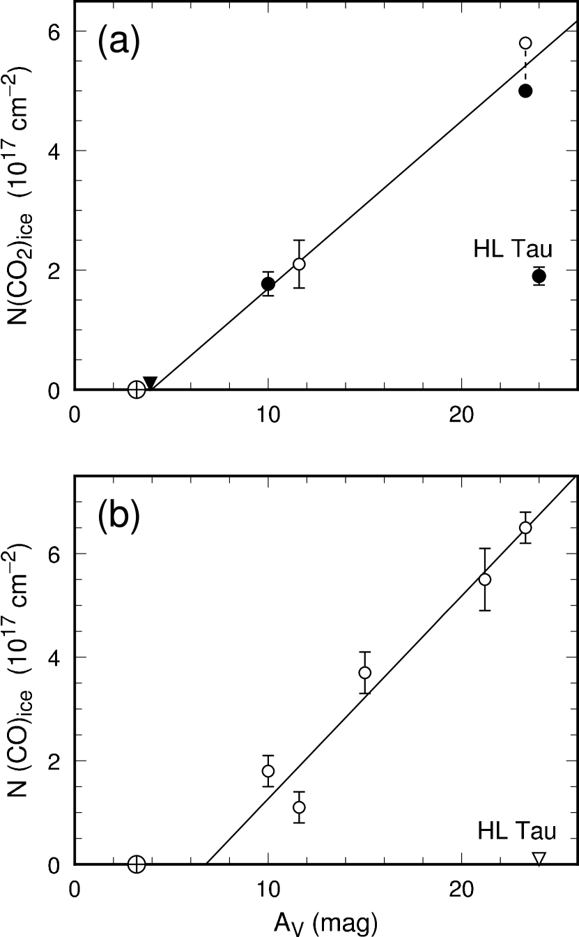
Figure 3: Plots of ice column density vs. visual extinction for (a) CO₂ and (b) CO. Open and filled symbols in (a) represent stretching and bending vibrational modes of CO₂, observed with the ISO SWS (Gerakines et al.  1999; Nummelin et al.  2001) and SST IRS (this paper), respectively. The points for one object (Elias 16) observed in both vibrational modes are joined by a vertical dashed line. Triangles indicate upper limits. The circled cross on the $A_{V}$ axis indicates the locus of the threshold extinction for H₂O-ice ($A_{V}=3.2$; Whittet et al.  2001). The diagonal line in each frame is the linear least-squares fit to field stars.

It is known from previous studies of ice features in Taurus that the absorption strength correlates with extinction. The correlation line intercepts the extinction axis at a positive value, i.e. there exists a threshold extinction below which the ice feature is not seen, presumably because the grains in the more diffuse outer layers of the cloud are not mantled (e.g. Chiar et al.  1995, Whittet et al.  2001 and references therein). Figure 3 compares plots of column density vs. extinction for CO₂ and CO. In the case of CO₂, we combine both Spitzer and ISO observations. The field-star data suggest a correlation yielding a threshold extinction $A_{V}=4^{m}\pm 1^{m}$, i.e. not significantly different from the value of $3.2^{m}\pm 0.1^{m}$ reported for water-ice (Whittet et al.  2001). In contrast, the threshold estimated for CO ($6.8^{m}\pm 1.6^{m}$) appears to be significantly larger. These results are consistent with a model in which most of the CO₂ is in the polar H₂O-rich component, whereas most of the CO is in the apolar, H₂O-poor component. A larger threshold is expected for the latter because of its greater volatility, requiring a greater degree of screening from the external radiation field.

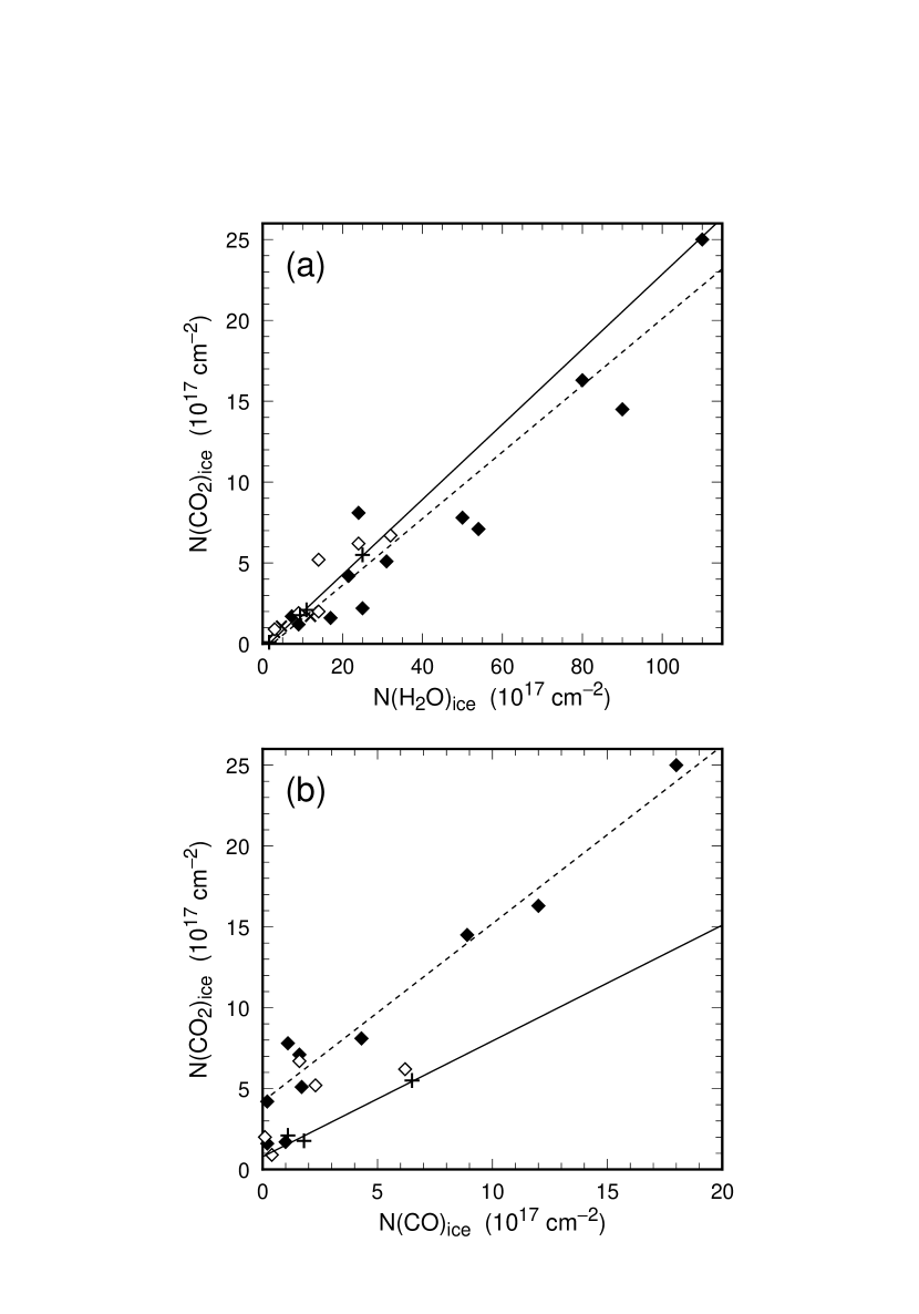
Figure 4: Plots of $N$(CO₂) vs.(a) $N$(H₂O) and (b) $N$(CO) for all sources with data available from SST (this paper) or ISO SWS (Gerakines et al.  1999; Nummelin et al.  2001). The symbols have the following meanings: Taurus field stars ($+$); Galactic Center field stars ($\times$); low-mass YSOs (open diamonds); high-mass YSOs (solid diamonds). The solid diagonal line in each frame is the linear least-squares fit to field stars. The dashed line in (a) is the fit to YSOs only (both high and low mass). The dashed line in (b) is the relation $N({\rm CO_{2}})=4.2\times 10^{17}+1.1N({\rm CO})$ proposed by Gerakines et al.  (1999) for high-mass YSOs.

Figure 4 plots ice-phase column densities for CO₂ vs. H₂O and CO. In the case of CO₂ vs. H₂O, there is a general trend – linear least-squares fits to field stars and YSOs are similar and intercept close to the origin. In contrast, the CO₂ vs. CO plot shows a tendency to divide into two distinct trends (Gerakines et al.  1999). For a given CO ice column, field stars have a lower CO₂ ice column than massive YSOs. Grains in front of field stars are covered by polar and apolar mantles. In contrast, in the warm envelopes of massive YSOs, the dominant factor is likely to be sublimation of apolar CO-rich ices (although some CO₂ might also be produced by energetic processes). The lower-mass YSOs show an intermediate distribution.

5 Implications for CO₂ Ice Formation

The Spitzer data on field stars revealed that (1) most of the CO₂ ice is embedded within the water ice mantle and (2) the CO₂ extinction threshold is closer to the threshold for water ice than that of its presumed precursor molecule, CO. These two results strongly suggest that CO₂ ice formation occurs in tandem with that of water ice. Water ice is believed to form via surface reactions during phases when gas is rich in atomic hydrogen and atomic oxygen. Observations of water vapor imply that atomic oxygen must be depleted in dense evolved well shielded molecular regions; the low abundance of gas-phase water inferred by SWAS (Snell et al. 2000) and ODIN (Olofsson et al. 2003) can only be accounted for in models where nearly all available gas-phase atomic oxygen becomes locked on grains (Bergin et al. 2000).

Thus H₂O and CO₂ ice formation must occur during the early lower density formative stages of the cloud. Recent models of molecular cloud formation behind shock waves by Bergin et al. (2004) may therefore be useful in setting constraints on ice formation. They found that H₂ formation occurs at earlier times than gas-phase CO formation because H₂ efficiently self-shields while CO formation requires dust shielding (A${}_{V}\sim 0.7$ mag). At such low cloud depths ice mantle formation would be retarded by UV photodesorption. However, for A_V $>1.0^{m}$ the effects of photodesorption are greatly reduced. In this scenario CO gas-phase formation precedes both CO and water ice mantle formation. This qualitatively answers several questions. Because most available gas-phase carbon would be locked in gas-phase CO, it would preclude a high abundance of methane ice, in accord with observations (Gibb et al., 2004b). It also allows for H, O, and CO to be present on the grain surface to react via simple catalytic reactions to create H₂O and CO₂.

One key question remains: how to account for the presence of apolar CO₂ ice? If CO₂ forms in tandem with H₂O in oxygen rich gas then how is a separate component of CO₂ formed with little H₂O? This implies the presence of O I in gas with little H I. There are at least 2 scenarios that could account for this mantle structure: line of sight structure in the abundance of atomic hydrogen or atomic oxygen (or perhaps both). To examine the question of line of sight structure in atomic hydrogen, in Elias 16 the abundance of CO₂ in the apolar mantle is $\sim 3\times 10^{-6}$ (all abundances relative to H₂): thus gas-phase H I would need to fall below this value to stop O I hydrogenation. Atomic hydrogen is expected to have near constant space density in molecular clouds, $n_{\rm{H\,I}}\sim 1-5$ cm^-3 (see Goldsmith & Li 2005). Thus, the H I abundance should inversely follow density variations along the Elias 16 line of sight. However, the density would need to be $>10^{6}$ cm^-3 for the abundance of H I to fall below that required for O I. This density is characteristic of a condensed molecular core, which is not detected towards this line of sight (Cernicharo & Guelin, 1987), and is therefore implausibly high. Thus H I abundance structure is insufficient to account for apolar CO₂.

Line of sight structure in the O I abundance provides a more plausible solution to this issue. If atomic oxygen were absent in the densest regions with high extinction, by water ice formation and other additional solid-state reservoirs, then oxygen hydrogenation could have halted in these regions. Oxidation could continue in layers with lower extinction and density. For instance, assuming a density of 10⁴ cm^-3 for the Elias 16 line of sight (Bergin et al., 1995), the atomic oxygen abundance would need to be $\gtrsim 10^{-4}$ to be higher than H I, which is conceivable given the available O I ($\sim 8\times 10^{-4}$; Jensen et al., 2005). Thus CO oxidation could continue in outer layers rich in atomic oxygen. There is some evidence for large O I columns towards molecular clouds that may trace low density layers (Caux et al., 1999; Lis et al., 2001; Li et al., 2002, and references therein). This qualitative model can be tested by future higher signal-to-noise Spitzer observations of low extinction field stars (e.g. Elias 3). For instance, line of sight structure in the oxygen abundance would predict the existence of apolar CO₂ at moderate optical depths, even at those below the CO ice threshold. Alternately, under the assumption that lower A_V implies lower density, then decreasing amounts of apolar CO₂ would suggest a relation to the declining abundance of atomic hydrogen with increasing density.

Figure 1: Spitzer IRS Short-HI spectra towards background stars Tamura 17, Elias 3, and Elias 16; HL Tau is a Class I pre-main sequence star. These spectra are shown without any baseline subtraction.

Figure 2: Optical depth of CO₂ ice absorption seen towards Elias 16 (histogram). Best fit line profile using laboratory analogs of interstellar ice mixtures at 10 K (solid line). The best fit requires two components: CO₂ embedded in a water rich (polar) mantle, shown as the short-dashed line (laboratory ice analog mixture H₂O $+$ CO₂ 100:14). The second component, shown as long-dashed line is CO₂ embedded in an apolar mantle (laboratory ice analog mixture CO $+$ CO₂ 100:26).

Table 1: Observation Parameters and Results

Source	Obs. Date	$\int\tau(\tilde{\nu})\Delta\tilde{\nu}$	N(CO2)	$\rm{\frac{N(CO_{2})}{N(H_{2}O)}}$	$\rm{\frac{N(CO_{2})}{N(CO)}}$	AV
Elias 16	Mar. 3, 2004	5.0$\pm$0.1	5.0	0.21	0.8	23.3m
Elias 3	Mar. 3, 2004	1.8$\pm$0.1	1.8	0.20	1.0	10.0m
Tamura 17	Feb. 27, 2004	$<$0.1(3$\sigma$)	$<$0.12	$<$0.10	$\cdots$	3.9m
HL Tau	Oct. 10, 2004	1.9$\pm$0.1	1.9	0.14	$\cdots$	24.0m

Note. — $N$(CO) data for field stars and the limiting value for HL Tau are from Chiar et al.  (1995) and Tegler et al.  (1995), respectively. The $A_{V}$ value for HL Tau is from Close et al.  (1997), those for field stars are calculated from the $J-K$ color excess assuming $A_{V}=5.3E_{J-K}$ (Whittet et al.  2001).

References

- Bergin et al. (2004) Bergin, E. A., Hartmann, L. W., Raymond, J. C., & Ballesteros-Paredes, J. 2004, ApJ, 612, 921
- Bergin et al. (2000) Bergin, E. A., et al. 2000, ApJ, 539, L129
- Bergin et al. (1995) Bergin, E. A., Langer, W. D., & Goldsmith, P. F. 1995, ApJ, 441, 222
- Caux et al. (1999) Caux, E., et al. 1999, A&A, 347, L1
- Cernicharo & Guelin (1987) Cernicharo, J., & Guelin, M. 1987, A&A, 176, 299
- Chiar et al. (1996) Chiar, J. E., Adamson, A. J., & Whittet, D. C. B. 1996, ApJ, 472, 665
- Chiar et al. (1995) Chiar, J. E., Adamson, A. J., Kerr, T. H., & Whittet, D. C. B. 1995, ApJ, 455, 234
- Close et al. (1997) Close, L. M., Roddier, F., Northcott, M. J., Roddier, C., & Graves, J. E. 1997, ApJ, 478, 766
- Dhendecourt et al. (1986) D’Hendecourt, L. B., Allamandola, L. J., Grim, R. J. A., & Greenberg, J. M. 1986, A&A, 158, 119
- Ehrenfreund et al. (1997) Ehrenfreund, P., Boogert, A. C. A., Gerakines, P. A., Tielens, A. G. G. M., & van Dishoeck, E. F. 1997, A&A, 328, 649
- Ehrenfreund et al. (1996) Ehrenfreund, P. et al. 1996, A&A, 315, L341
- Frost et at. (1991) Frost, M.J., Sharkey, P., & Smith, I.M. 1991, Faraday Discuss., 91, 305
- Gerakines et al. (1999) Gerakines, P. A., et al. 1999, ApJ, 522, 357
- Gerakines et al. (1995) Gerakines, P. A., Schutte, W. A., Greenberg, J. M., & van Dishoeck, E. F. 1995, A&A, 296, 810
- Gibb et al. (2004a) Gibb, E. L., Rettig, T., Brittain, S., Haywood, R., Simon, T., & Kulesa, C. 2004b, ApJ, 610, L113
- Gibb et al. (2004b) Gibb, E. L., Whittet, D. C. B., Boogert, A. C. A., & Tielens, A. G. G. M. 2004a, ApJS, 151, 35
- Goldsmith et al. (2000) Goldsmith, P. F., et al. 2000, ApJ, 539, L123
- Goldsmith & Li (2005) Goldsmith, P. F., & Li, D. 2005, ApJ, 622, 938
- Higdon et al. (2004) Higdon, S. J. U., et al. 2004, PASP, 116, 975
- Hiraoka et al. (2005) Hiraoka, K., et al. 2005, ApJ, 620, 542
- Houck et al. (2004) Houck, J. R., et al. 2004, ApJS, 154, 18
- Jensen et al. (2005) Jensen, A. G., Rachford, B. L., & Snow, T. P. 2005, ApJ, 619, 891
- Li et al. (2002) Li, W., Evans, N. J., Jaffe, D. T., van Dishoeck, E. F., & Thi, W. 2002, ApJ, 568, 242
- Lis et al. (2001) Lis, D. C., Keene, J., Phillips, T. G., Schilke, P., Werner, M. W., & Zmuidzinas, J. 2001, ApJ, 561, 823
- Nummelin et al. (2001) Nummelin, A., Whittet, D. C. B., Gibb, E. L., Gerakines, P. A., & Chiar, J. E. 2001, ApJ, 558, 185
- Olofsson et al. (2003) Olofsson, A. O. H., et al. 2003, A&A, 402, L47
- Pagani et al. (2003) Pagani, L., et al. 2003, A&A, 402, L77
- Palumbo et al. (1998) Palumbo, M. E., et al. 1998, A&A, 334, 247
- Roser et al. (2001) Roser, J. E., Vidali, G., Manicò, G., & Pirronello, V. 2001, ApJ, 555, L61
- Sandford et al. (1988) Sandford, S. A., Allamandola, L. J., Tielens, A. G. G. M., & Valero, G. J. 1988, ApJ, 329, 498
- Sandford & Allamandola (1990) Sandford, S. A., & Allamandola, L. J. 1990, Icarus, 87, 188
- Snell et al. (2000) Snell, R. L., et al. 2000, ApJ, 539, L101
- Tegler et al. (1995) Tegler, S. C. et al. 1995, ApJ, 439, 279
- Vandenbussche et al. (1999) Vandenbussche, B., et al. 1999, A&A, 346, L57
- van Dishoeck (2004) van Dishoeck, E. F. 2004, ARA&A, 42, 119
- Watson et al. (2004) Watson, D. M., et al. 2004, ApJS, 154, 391
- Whittet et al. (2001) Whittet, D. C. B., Gerakines, P. A., Hough, J. H., & Shenoy, S. S. 2001, ApJ, 547, 872
- Whittet et al. (1998) Whittet, D. C. B., et al. 1998, ApJ, 498, L159