A Multi-wavelength View of the TeV Blazar Markarian 421: Correlated Variability, Flaring, and Spectral Evolution

M. Błażejowski¹¹affiliation: Department of Physics, Purdue University, West Lafayette, IN 47907, USA , G. Blaylock²²affiliation: Department of Physics, University of Massachusetts, Amherst, MA 01003, USA , I. H. Bond³³affiliation: Department of Physics, University of Leeds, Leeds, LS2 9JT, Yorkshire, England, UK , S. M. Bradbury³³affiliation: Department of Physics, University of Leeds, Leeds, LS2 9JT, Yorkshire, England, UK , J. H. Buckley⁴⁴affiliation: Department of Physics, Washington University, St. Louis, MO 63130, USA , D. A. Carter-Lewis⁵⁵affiliation: Department of Physics and Astronomy, Iowa State University, Ames, IA 50011, USA , O. Celik⁶⁶affiliation: Department of Physics, University of California, Los Angeles, CA 90095, USA , P. Cogan⁷⁷affiliation: Physics Department, National University of Ireland, Belfield, Dublin 4, Ireland , W. Cui¹¹affiliation: Department of Physics, Purdue University, West Lafayette, IN 47907, USA , M. Daniel⁷⁷affiliation: Physics Department, National University of Ireland, Belfield, Dublin 4, Ireland , C. Duke⁸⁸affiliation: Physics Department, Grinnell College, Grinnell, IA 50112, USA , A. Falcone¹¹affiliation: Department of Physics, Purdue University, West Lafayette, IN 47907, USA , D. J. Fegan⁷⁷affiliation: Physics Department, National University of Ireland, Belfield, Dublin 4, Ireland , S. J. Fegan⁶⁶affiliation: Department of Physics, University of California, Los Angeles, CA 90095, USA , J. P. Finley¹¹affiliation: Department of Physics, Purdue University, West Lafayette, IN 47907, USA , L. Fortson⁹⁹affiliation: Adler Planetarium and Astronomy Museum, Astronomy Department, Chicago, IL 60605 , S. Gammell⁷⁷affiliation: Physics Department, National University of Ireland, Belfield, Dublin 4, Ireland , K. Gibbs¹⁰¹⁰affiliation: Fred Lawrence Whipple Observatory, Harvard-Smithsonian Center for Astrophysics, Amado, AZ 85645, USA , G. G. Gillanders¹¹¹¹affiliation: Physics Department, National University of Ireland, Galway, Ireland , J. Grube³³affiliation: Department of Physics, University of Leeds, Leeds, LS2 9JT, Yorkshire, England, UK , K. Gutierrez⁴⁴affiliation: Department of Physics, Washington University, St. Louis, MO 63130, USA , J. Hall¹²¹²affiliation: High Energy Astrophysics Institute, University of Utah, Salt Lake City, UT 84112, USA , D. Hanna¹³¹³affiliation: Physics Department, McGill University, Montreal, QC H3A 2T8, Canada , J. Holder³³affiliation: Department of Physics, University of Leeds, Leeds, LS2 9JT, Yorkshire, England, UK , D. Horan¹⁰¹⁰affiliation: Fred Lawrence Whipple Observatory, Harvard-Smithsonian Center for Astrophysics, Amado, AZ 85645, USA , B. Humensky¹⁴¹⁴affiliation: Enrico Fermi Institute, University of Chicago, Chicago, IL 60637, USA , G. Kenny¹¹¹¹affiliation: Physics Department, National University of Ireland, Galway, Ireland , M. Kertzman¹⁵¹⁵affiliation: Physics Department, DePauw University, Greencastle, IN, 46135, USA , D. Kieda¹²¹²affiliation: High Energy Astrophysics Institute, University of Utah, Salt Lake City, UT 84112, USA , J. Kildea¹³¹³affiliation: Physics Department, McGill University, Montreal, QC H3A 2T8, Canada , J. Knapp³³affiliation: Department of Physics, University of Leeds, Leeds, LS2 9JT, Yorkshire, England, UK , K. Kosack⁴⁴affiliation: Department of Physics, Washington University, St. Louis, MO 63130, USA , H. Krawczynski⁴⁴affiliation: Department of Physics, Washington University, St. Louis, MO 63130, USA , F. Krennrich⁵⁵affiliation: Department of Physics and Astronomy, Iowa State University, Ames, IA 50011, USA , M. Lang¹¹¹¹affiliation: Physics Department, National University of Ireland, Galway, Ireland , S. LeBohec¹²¹²affiliation: High Energy Astrophysics Institute, University of Utah, Salt Lake City, UT 84112, USA , E. Linton¹⁴¹⁴affiliation: Enrico Fermi Institute, University of Chicago, Chicago, IL 60637, USA , J. Lloyd-Evans³³affiliation: Department of Physics, University of Leeds, Leeds, LS2 9JT, Yorkshire, England, UK , G. Maier³³affiliation: Department of Physics, University of Leeds, Leeds, LS2 9JT, Yorkshire, England, UK , D. Mendoza¹¹affiliation: Department of Physics, Purdue University, West Lafayette, IN 47907, USA , A. Milovanovic³³affiliation: Department of Physics, University of Leeds, Leeds, LS2 9JT, Yorkshire, England, UK , P. Moriarty¹⁶¹⁶affiliation: School of Physical Sciences, Galway-Mayo Institute of Technology, Galway, Ireland , T. N. Nagai¹²¹²affiliation: High Energy Astrophysics Institute, University of Utah, Salt Lake City, UT 84112, USA , R. A. Ong⁶⁶affiliation: Department of Physics, University of California, Los Angeles, CA 90095, USA , B. Power-Mooney⁷⁷affiliation: Physics Department, National University of Ireland, Belfield, Dublin 4, Ireland , J. Quinn⁷⁷affiliation: Physics Department, National University of Ireland, Belfield, Dublin 4, Ireland , M. Quinn¹⁶¹⁶affiliation: School of Physical Sciences, Galway-Mayo Institute of Technology, Galway, Ireland , K. Ragan¹³¹³affiliation: Physics Department, McGill University, Montreal, QC H3A 2T8, Canada , P. T. Reynolds¹⁷¹⁷affiliation: Department of Applied Physics and Instrumentation, Cork Institute of Technology, Cork, Ireland , P. Rebillot⁴⁴affiliation: Department of Physics, Washington University, St. Louis, MO 63130, USA , H. J. Rose³³affiliation: Department of Physics, University of Leeds, Leeds, LS2 9JT, Yorkshire, England, UK , M. Schroedter⁵⁵affiliation: Department of Physics and Astronomy, Iowa State University, Ames, IA 50011, USA , G. H. Sembroski¹¹affiliation: Department of Physics, Purdue University, West Lafayette, IN 47907, USA , S. P. Swordy¹⁴¹⁴affiliation: Enrico Fermi Institute, University of Chicago, Chicago, IL 60637, USA , A. Syson³³affiliation: Department of Physics, University of Leeds, Leeds, LS2 9JT, Yorkshire, England, UK , L. Valcarel¹³¹³affiliation: Physics Department, McGill University, Montreal, QC H3A 2T8, Canada , V. V. Vassiliev⁶⁶affiliation: Department of Physics, University of California, Los Angeles, CA 90095, USA , S. P. Wakely¹⁴¹⁴affiliation: Enrico Fermi Institute, University of Chicago, Chicago, IL 60637, USA , G. Walker¹²¹²affiliation: High Energy Astrophysics Institute, University of Utah, Salt Lake City, UT 84112, USA , T. C. Weekes¹⁰¹⁰affiliation: Fred Lawrence Whipple Observatory, Harvard-Smithsonian Center for Astrophysics, Amado, AZ 85645, USA , R. White³³affiliation: Department of Physics, University of Leeds, Leeds, LS2 9JT, Yorkshire, England, UK , and J. Zweerink⁶⁶affiliation: Department of Physics, University of California, Los Angeles, CA 90095, USA ,
and
B. Mochejska¹¹affiliation: Department of Physics, Purdue University, West Lafayette, IN 47907, USA , B. Smith¹¹affiliation: Department of Physics, Purdue University, West Lafayette, IN 47907, USA , M. Aller¹⁸¹⁸affiliation: Department of Astronomy, University of Michigan, Ann Arbor, MI 48109, USA , H. Aller¹⁸¹⁸affiliation: Department of Astronomy, University of Michigan, Ann Arbor, MI 48109, USA , H. Teräsranta¹⁹¹⁹affiliation: Metsähovi Radio Observatory, Helsinki University of Technology, Mesähovintie 114, 02540 Kylmälä, Finland , P. Boltwood²⁰²⁰affiliation: Boltwood Observatory, 1655 Main Street, Stittsville, Ont. K2S 1N6, Canada , A. Sadun²¹²¹affiliation: Department of Physics, University of Colorado at Denver, CO 80217, USA , K. Stanek²²²²affiliation: Harvard-Smithsonian Center for Astrophysics, 60 Garden Street, Cambridge, MA 02138, USA , E. Adams²²²²affiliation: Harvard-Smithsonian Center for Astrophysics, 60 Garden Street, Cambridge, MA 02138, USA , J. Foster²²²²affiliation: Harvard-Smithsonian Center for Astrophysics, 60 Garden Street, Cambridge, MA 02138, USA , J. Hartman²²²²affiliation: Harvard-Smithsonian Center for Astrophysics, 60 Garden Street, Cambridge, MA 02138, USA , K. Lai²²²²affiliation: Harvard-Smithsonian Center for Astrophysics, 60 Garden Street, Cambridge, MA 02138, USA , M. Böttcher²³²³affiliation: Department of Astronomy, Ohio University, Athens, OH 05701, USA , A. Reimer²⁴²⁴affiliation: Institut für Theoretische Physik, Lehrstuhl IV: Weltraum und Astrophysik, Ruhr-Universität Bochum, D 44780 Bochum, Germany , and I. Jung⁴⁴affiliation: Department of Physics, Washington University, St. Louis, MO 63130, USA

Abstract

We report results from an intensive multi-wavelength monitoring campaign on the TeV blazar Mrk 421 over the period of 2003–2004. The source was observed simultaneously at TeV energies with the Whipple 10 m telescope and at X-ray energies with Rossi X-ray Timing Explorer (RXTE) during each clear night within the Whipple observing windows. Supporting observations were also frequently carried out at optical and radio wavelengths to provide simultaneous or contemporaneous coverages. The large amount of simultaneous data has allowed us to examine the variability of Mrk 421 in detail, including cross-band correlation and broad-band spectral variability, over a wide range of flux. The variabilities are generally correlated between the X-ray and gamma-ray bands, although the correlation appears to be fairly loose. The light curves show the presence of flares with varying amplitudes on a wide range of timescales both at X-ray and TeV energies. Of particular interest is the presence of TeV flares that have no coincident counterparts at longer wavelengths, because the phenomenon seems difficult to understand in the context of the proposed emission models for TeV blazars. We have also found that the TeV flux reached its peak days before the X-ray flux did during a giant flare (or outburst) in 2004 (with the peak flux reaching $\sim$ 135 mCrab in X-rays, as seen by the ASM/RXTE, and $\sim$ 3 Crab in gamma rays). Such a difference in the development of the flare presents a further challenge to the leptonic and hadronic emission models alike. Mrk 421 varied much less at optical and radio wavelengths. Surprisingly, the normalized variability amplitude in optical seems to be comparable to that in radio, perhaps suggesting the presence of different populations of emitting electrons in the jet. The spectral energy distribution of Mrk 421 is seen to vary with flux, with the two characteristic peaks moving toward higher energies at higher fluxes. We have failed to fit the measured SEDs with a one-zone SSC model; introducing additional zones greatly improves the fits. We have derived constraints on the physical properties of the X-ray/gamma-ray flaring regions from the observed variability (and SED) of the source. The implications of the results are discussed.

BL Lacertae objects: individual (Markarian 421) – galaxies: active — galaxies: jets – gamma rays: observations — radiation mechanisms: non-thermal — X-rays: galaxies

1 Introduction

Over the past decade or so, one of the most exciting advances in high energy astrophysics has been the detection of sources at TeV energies with ground-based gamma ray facilities (see Weekes 2003 for a recent review). Among the sources detected, blazars are arguably the most intriguing. They represent the only type of active galactic nuclei (AGN) that has been detected at TeV energies (although a 4- $\sigma$ detection of M87 has been reported; Aharonian et al. 2003). To date, there are a total of six firmly established TeV blazars.

The emission from a blazar is generally thought to be dominated by radiation from a relativistic jet that is directed roughly along the line of sight (review by Urry & Padovani 1995 and references therein). Relativistic beaming is necessary to keep gamma-ray photons from being significantly attenuated by the surrounding radiation field (via photon-photon pair production). The spectral energy distribution (SED) of TeV blazars invariably shows two characteristic peaks in the $\nu F_{\nu}$ representation, with one located at X-ray energies and the other at TeV energies (Fossati et al. 1998). There seems to be a general correlation between the two SED peaks as the source varies (e.g., Buckley et al. 1996; Catanese et al. 1997; Maraschi et al. 1999; Petry et al. 2000).

A popular class of models associates the X-ray emission from a TeV blazar with synchrotron radiation from highly relativistic electrons in the jet and the TeV emission with inverse-Compton scattering of the synchrotron photons by the electrons themselves (i.e., synchrotron self-Compton or SSC for short; Marscher & Gear 1985; Maraschi et al. 1992; Dermer et al. 1992; Sikora et al. 1994; see Böttcher 2002 for a recent review). The SSC models can, therefore, naturally account for the observed X-ray–TeV correlation. Moreover, they have also enjoyed some success in reproducing the measured SEDs. However, the models still face challenges in explaining some of the observed phenomena, such as the presence of “orphan” TeV flares (Krawczynski et al. 2004; Cui et al. 2004).

Alternatively, the jet might be energetically dominated by the magnetic field and it is the synchrotron radiation from highly relativistic protons that might be responsible for the observed TeV gamma rays (Aharonian 2000; Mücke et al. 2003). Other hadronic processes have also been considered, including photo-meson production, neutral pion decay, and synchrotron-pair cascading (e.g., Mannheim & Biermann 1992; Mücke et al. 2003), but they are thought to be less important in TeV blazars (Aharonian 2000; Mücke et al. 2003). Another class of hadronic models invokes $pp$ processes, for instance, in the collision between the jet and ambient “clouds” (e.g., Dar & Laor 1997; Beall & Bednarek 1999) or inside the (dense) jet (Pohl & Schlickeiser 2000). In this case, the gamma-ray emission is mainly attributed to the decay of neutral pions produced in the $pp$ interactions. In both classes of hadronic models, the emission at X-ray and longer wavelengths is still attributed to the synchrotron radiation from relativistic electrons (and positrons) in the jet, as in the SSC models. Although the hadronic models may also be able to describe the observed SED of TeV blazars and accommodate the X-ray–TeV correlation, they are generally challenged by the most rapid gamma-ray variabilities observed in TeV blazars (Gaidos et al. 1996).

TeV blazars are also known to undergo flaring episodes both at X-ray and TeV energies. The flares have been observed over a wide range of timescales, from months down to less than an hour. The observed X-ray flaring hierarchy seems to imply a scale-invariant physical origin of the flares (Cui 2004; Xue & Cui 2005). Blazar flares are thought to be related to internal shocks in the jet (Rees 1978; Spada et al. 2001), or to the ejection of relativistic plasma into the jet (e.g., Böttcher et al. 1997; Mastichiadis & Kirk 1997). Recently, it is suggested that the flares could also be associated with magnetic reconnection events in a magnetically dominated jet (Lyutikov 2003) and thus they could be similar to solar flares in this regard. Such a model might offer a natural explanation for the hierarchical flaring phenomenon, again in analogy to solar flares.

To make further progress on distinguishing the emission models proposed for TeV blazars, we believe that a large amount of simultaneous or contemporaneous data is critically needed over a wide range of flux, especially in the crucial X-ray and TeV bands, for quantifying the SED and spectral variability of a source and for allowing investigations of such important issues as variability timescales, cross-band correlation, spectral variability, spectral hysteresis, etc. Such data are severely lacking at present, despite intense observational efforts over the years. In this paper, we present results from an intensive multi-wavelength monitoring campaign on Mrk 421. This source is the first TeV blazar discovered (Punch et al. 1992) and remains one of the few blazars that can be detected at TeV energies nearly all the time with ground-based imaging atmospheric Cherenkov telescopes (IACTs). Some of the preliminary results have appeared elsewhere (Cui et al. 2004); they are superseded by those presented in this work.

We have assumed the following values for the various cosmological parameters: $H=71\mbox{ }km\mbox{ }s^{-1}\mbox{ }Mpc^{-1}$ , $\Omega_{m}=0.27$ , and $\Omega_{\Lambda}=0.73$ . The corresponding luminosity distance of Mrk 421 ( $z=0.031$ ) is about 129.8 Mpc.

2 Observations and Data Reduction

2.1 Gamma-ray Observations

From 2003 February to 2004 June, Mrk 421 was observed at TeV energies with the Whipple 10 m Telescope (on Mt. Hopkins, AZ) during each clear night within the dark moon observing periods. The typical exposure time of a nightly observation was 28 minutes, corresponding to one observing run, but more runs were taken on occasion, especially near the end of the campaign (in 2004 April) when the source was seen to undergo an usually large X-ray outburst as seen by the All-Sky Monitor (ASM) on RXTE. To achieve simultaneous coverages of the source both in the TeV and X-ray bands, we communicated with the RXTE Science Operations Facility to ensure that the Whipple and RXTE observing schedules were matched as closely as possible. A total of 306 runs were collected in good (empirically designated as “A” or “B”) weather, and roughly 80% of them were taken at zenith angles $\lesssim$ 30°.

The procedure for reducing and analyzing Whipple data has been standardized over the years (Hillas 1985; Reynolds et al. 1993; Mohanty et al. 1998). A detailed description of the current hardware can be found in Finley et al. (2001). For clarity, we briefly summarize a few key points that are relevant to this work. The success of IACTs lies in the fact that the Cherenkov images of an air shower produced by a gamma-ray primary have different shapes and orientations than those found in an air shower produced by cosmic-ray particles (mostly protons). The images in gamma-ray events are typically more compact and are more aligned to point towards the position of the source than those in cosmic-ray events. In practice, the image shape of an event is characterized by the major and minor axes of the best-fit ellipse to the image. The orientation of the ellipse is characterized by the parameter ” $\alpha$ ”, defined as the angle between the major axis and the line connecting the center of the ellipse to the center of the field-of-view (FOV). We have developed standard selection criteria based primarily on the image shape and orientation parameters that remove over 99% of the cosmic ray events while keeping about half of the gamma-ray events (see, e.g., Falcone et al. 2004 for more details).

The Whipple observations are conducted in one of the two modes: tracking and ON/OFF. In the tracking mode, the telescope tracks the target across the sky so that the source stays at the center of the FOV throughout the observation. In the ON/OFF mode, on the other hand, the telescope tracks the target only during the ON run; it is then offset by 30 minutes in right ascension during the OFF run, and tracks the field as it covers the same range of zenith and azimuthal angles. The OFF run provides a direct measurement of the background, although the difference in the sky brightness of the fields between the ON and OFF runs must be taken into account by using a technique known as software padding (Reynolds et al 1993). For tracking observations, the background is derived from the $\alpha$ histogram of the events that have passed all but the orientation cuts. Since real gamma-ray events from a source should all be concentrated at small $\alpha$ values ( $<$ 15°) for on-axis observations, the background level can be estimated from events with larger $\alpha$ values (20°–65°), if the ratio of the number of background events in the two ranges of the $\alpha$ parameter is known. This ratio is derived from observations of fields in which there is no evidence for a gamma-ray source (see, e.g., Falcone et al. 2004).

Nearly all of the Whipple observations reported in this work were carried out in the tracking mode. We followed the standard procedure just described to obtain count rates from individual runs (taken in the good weather) and thus the long-term light curves. To examine variability on short timescales, we sometimes sub-divided runs into time intervals shorter than the nominal 28 minutes and constructed light curves with correspondingly smaller time bins. To correct for the effects due to changes in the zenith angle and overall throughput of the telescope, we applied the method developed by LeBohec & Holder (2003) to the data. We should note that for a given season the corrections were made with respect to a (somewhat arbitrarily chosen) reference run taken at 30° zenith angle during a clear night. To correct for changes in the telescope throughput across seasons, we used the measured rates for the Crab Nebula to further calibrate the light curves. For reference, the rate of the Crab Nebula is about 2.40 and 2.93 $\gamma\mbox{ }min^{-1}$ for the 2002/2003 and 2003/2004 seasons, respectively.

The spectral analysis was carried out by following Method 1 described in Mohanty et al. (1998). The technical aspects and difficulties involved in finding matching pairs for the spectral analysis of tracking observations are explained in detail by Petry et al. (2002) and Daniel et al. (2005). Combined with the fact that the observations were taken only in the tracking mode, poor statistics made it extremely challenging to derive a TeV spectrum from observations taken at low fluxes. For those cases, the tolerance for the parameter cuts was tightened to be just 1.5 standard deviations from the average value of the simulations, as opposed to the usual 2 standard deviations, in order to further reduce the cosmic-ray background (Daniel et al. 2005). The tighter cuts still retained $\sim 80\%$ of gamma rays. The downside is that the effective collection area of the telescope is not as independent of energy as can be ideally hoped for (Mohanty et al. 1998).

2.2 X-ray observations

In coordination with each Whipple observation, we took a snapshot of Mrk 421 at X-ray energies with RXTE (with a typical exposure time of 2–3 ks). We should note, however, that not every X-ray observation was accompanied by a simultaneous Whipple observation (due, e.g., to poor weather) and vice versa (especially near the end of the campaign, when many more Whipple observations were made to monitor the source in an exceptionally bright state; see Fig. 1). For this work, we only used data from the PCA instrument on RXTE, which covers a nominal energy range of 2–60 keV. The PCA consists of five nearly identical proportional counter units (PCUs). However, only two of the PCUs, PCU 0 and PCU 2, were in use throughout our campaign, due to operational constraints. PCU 0 has lost its front veto layer, so the data from it are more prone to contamination by events caused by low-energy electrons entering the detector. The problem is particularly relevant to variability studies of relatively weak sources, such as Mrk 421. For this work, therefore, we have chosen PCU 2 as our “standard” detector for flux normalization and spectral analysis.

We followed Cui (2004) closely in reducing and analyzing the PCA data. Briefly, the data were reduced with FTOOLS 5.2. For a given observation, we first filtered data by following the standard procedure for faint sources,¹¹1See the online RXTE Cook Book, available at http://heasarc.gsfc.nasa.gov/docs/xte/recipes/cook_book.html. which resulted in a list of good time intervals (GTIs). We then simulated background events for the observation by using the latest background model that is appropriate for faint sources. Using the GTIs, we proceeded to extract a light curve for each PCU separately. We repeated the steps to construct the corresponding background light curves from the simulated events. We then subtracted the background from the total to obtain the light curves of the source. Following a similar procedure, for each observation, we also constructed the X-ray spectrum for each PCU and its associated background spectrum. In this case, however, we only used data from the first xenon layer of each PCU (which is most accurately calibrated), which limits the spectral coverage to roughly 2.5–25 keV. Since few counts were detected at higher energies, the impact of the reduced spectral coverage is very minimal.

2.3 Optical observations

The optical data were obtained with the Fred Lawrence Whipple Observatory (FLWO) 1.2 m telescope (located adjacent to the Whipple 10 m gamma-ray telescope on Mt. Hopkins) and with the 0.4 m telescope at the Boltwood Observatory in Stittsville, Ontario, Canada. We note that we had no optical coverage of the source during the 2002/2003 Whipple observing season.

The FLWO 1.2 m was equipped with 4Shooter CCD mosaic with four $2048\times 2048$ chips. Each chip covers a $11\farcm 4\times 11\farcm 4$ FOV. The data were collected during 31 nights, from 2003 December 14 to 2004 February 17. A total of 77 images were obtained in the $B$ band, 69 in the $V$ band, 67 in the $R$ band, and 78 in the $I$ band, with an exposure time of 30 s for each image. The preliminary processing of the CCD frames was performed with the standard routines in the IRAF ccdproc package.²²2IRAF is distributed by the National Optical Astronomy Observatories, which are operated by the Association of Universities for Research in Astronomy, Inc., under cooperative agreement with the NSF.

Photometry was extracted using the DAOphot/Allstar package (Stetson 1987). The fitting radius for profile photometry was varied with the seeing. The median seeing in our dataset was 4.5″. A detailed description of the applied procedure is given in § 3.2 of Mochejska et al. (2002). The derivation of photometry was complicated by the proximity of two very bright stars, HD 95934 (V=6 mag) and HD 95976 (V=7.5 mag), at angles of 2.1′ and 4′ from Mrk 421, respectively. These angles correspond to distances of 187 and 356 pixels on the images. The presence of these stars introduces a gradient in the background, approximately in the north-south direction. To estimate the magnitude of this gradient, we examined two $10\times 10$ pixel regions located at distances of 30–40 pixels north and south of Mrk 421. These regions were chosen to coincide with the annulus of 18-45 pixels used by Allstar for background determination. The difference in counts between the two regions is at a level of 1.4%, 0.7%, 0.3%, and 0.2% of the peak value of Mrk 421 with BVRI filters, respectively, on our best seeing images, and of 3.9%, 1.9%, 1.1%, and 0.6% on images with seeing close to the upper $85^{th}$ percentile. Thus, it varies with the seeing in BVRI by 2.5%, 1.2%, 0.8%, and 0.4%, respectively, all very small compared with the variability amplitudes of the source. The transformations of instrumental magnitudes to the standard system were derived from observations of 27 stars in 3 Landolt (1992) standard fields, collected on 19 January 2004. The systematic errors associated with the calibration are estimated to be 0.02 for BVI and 0.01 for R.

The Boltwood 0.4 m is equipped with an Apogee AP7p CCD camera that uses a back-illuminated SITE 502A chip. Mrk 421 was observed during the period from 2003 November 8 to 2004 June 11. The data were taken with an uncalibrated Cousins R filter (designed by Bessell and manufactured by Omega). The photometric measurements are differential (with respect to the comparison star 4 in Villata et al. 1998). Aperture photometry was performed with custom software. The aperture used is of 10″ in diameter. Data points were obtained from averaging over between four and six 2 minute exposures. The typical statistical error on the relative photometry of each data point is 0.02 in magnitude. The seeing-induced errors or other systematic errors were not taken into account. To cross check results from the two sets of measurements, we scaled up the Boltwood values (by adding a constant to the measured differential magnitudes) so that they agree, on average, with the FLWO fluxes for the overlapping time period. We found that the observed variation patterns agree quite well between the two data sets. This also implies that any variability caused by systematic effects must be small compared with the intrinsic variability of the source.

2.4 Radio observations

We observed Mrk 421 frequently with the 26-meter telescope at the University of Michigan Radio Astronomy Observatory (UMRAO) and the 13.7-meter Metsähovi radio telescope at the Helsinki University of Technology. The UMRAO telescope is equipped with transistor-based radiometers operating at center frequencies of 4.8, 8.0, and 14.5 GHz; their bandwidths are 560, 760, and 1600 MHz, respectively. All three frequencies utilize rotating, dual-horn polarimeter feed systems, which permit both total flux and linear polarizations to be measured using an ON-OFF observing technique at 4.8 GHz and an ON-ON technique (switching the target source between the two feed horns closely spaced on the sky) at the other two frequencies. The latter technique reduces the contribution of tropospheric interference by an order of magnitude. Observations of Mrk 421 were intermixed with observations of a grid of calibrator sources: 3C 274 is the most frequently used calibrator, except during a period each fall when the sun is within 15^∘ of the calibrator. The flux scale is set by observations of Cas A (e.g. see Baars et al. 1977). Details of the calibration and analysis techniques are described in Aller et al. (1985).

The Metsähovi observations were carried out as part of a long-time monitoring program. The observations were made with dual-horn receivers and the ON-ON technique, and they covered the 22 and 37 GHz bands. The flux measurements have been calibrated against DR 21 (with the adopted fluxes 19.0 and 17.9 Jy at 22 and 37 GHz, respectively). The full description of the receiving system can be found in Teräsranta et. al. (1998). The data were obtained during the period from 2003 January 1 to 2004 June 28.

3 Results

3.1 Light Curves

Figure 1 shows the light curves of Mrk 421 in the representative bands covered by the campaign. The source was relatively quiet during the 2002/2003 season, although it clearly varied at X-ray and TeV energies. The largest TeV flare occurred around MJD 52728 (= 30 March 2003), reaching a peak count rate of nearly 4 $\gamma\mbox{ }min^{-1}$ and lasting for about a week. The TeV flare was accompanied by a flare in X-rays, which reached a peak count rate of $\sim$ 65 $\mbox{ }cts\mbox{ }s^{-1}\mbox{ }PCU^{-1}$ (or about 24 mCrab). There is no apparent time offset between the X-ray and gamma-ray flares.

Mrk 421 became much more active in the 2003/2004 season, with several major flares observed. In particular, an usually large flare (or outburst) took place near the end of the campaign, with the source reaching peak fluxes of $\sim$ 135 mCrab in X-rays, as seen by the ASM/RXTE,³³3based on data from the MIT archive at http://xte.mit.edu/asmlc/srcs/mkn421.html#data and $\sim$ 3 Crabs in the TeV band, respectively. An expanded view of this flaring episode is shown in Figure 2. The flare lasted for more than two weeks (from $<$ MJD 53104 to roughly MJD 53120), although its exact duration is difficult to quantify due to the presence of a large data gap between MJD 53093 and MJD 53104. Interestingly, during this giant flare, the TeV emission appears to reach the peak much sooner than the X-ray emission. Although the X-ray light curve is not as densely sampled as the gamma-ray light curve, the fact that the X-ray measurements were made at the same time as the corresponding gamma-ray measurements (see Fig. 2) makes it quite unlikely that the difference in the rise time between the two bands is caused by some sampling bias.

The light curves also show that Mrk 421 varies much less at optical and radio wavelengths. The variability amplitude in the R band is less than about 0.9 magnitude; the variability is even less obvious in the radio bands due to relatively large measurement errors. There is no apparent correlation between the optical and radio bands or between either radio or optical band and the high-energy (X-ray and TeV) bands. For completeness, Figure 3 shows (FLWO) optical and radio light curves for all of the bands covered. The figure shows highly correlated variability among the optical bands, while the situation is not nearly as clear among the radio bands, due both to large measurement errors and sparse coverages.

3.1.1 Energy Dependence of the Source Variability

To quantify the energy dependence of variability amplitudes, we computed the so-called normalized variability amplitude (NVA) for each spectral band. The NVA is defined as (Edelson et al. 1996):

NVA\equiv\frac{{({\sigma_{tot}}^{2}-{\sigma_{err}}^{2})}^{1/2}}{\bar{F}},

where $\bar{F}$ represents the mean count rate or flux, $\sigma_{tot}$ the standard deviation, and ${\sigma_{err}}$ the mean measurement error in a given spectral band.

To facilitate comparison of the NVAs for different bands, we only used light curves that are relatively well sampled and cover the entire 2003/2004 season (see Fig. 1). Consequently, the results are obtained only for the following spectral bands: 14.5 GHz, R, X-ray, and gamma-ray. We first rebinned the selected light curves with the same bin size. To examine variabilities on different timescales, two different bin sizes were used: 1 day and 7 days. We then computed the NVAs from the rebinned light curves. The results are shown in Figure 4. The variability of Mrk 421 shows a general increasing trend toward high energies. The source is highly variable in the X-ray and TeV bands, with the NVA reaching up to about 65% (with 1-day binning), but varies much less in the radio and optical bands, with the NVA equal to $\sim$ 11% and $\sim$ 16%, respectively, almost independent of the binning schemes used.

There are several caveats in the cross-band comparison. First of all, the density of data sampling is quite different for different bands. For instance, the sampling is more sparse in the 14.5 GHz band than in any of the other bands. However, the under-sampling of the radio data would probably only lead to an under-estimation of the radio NVA. Secondly, the measurement errors for the optical data are probably underestimated, due to possible systematic effects caused by, e.g., the presence of bright stars in the field. This would result in an over-estimation of the optical NVA. Finally, the measured optical flux includes contribution from the host galaxy, which is at a $\sim$ 15% level (Nilsson et al. 1999). Since it only affects the average flux, not the absolute variability amplitude, the optical NVA should be about 15% higher, which is a small correction. Therefore, the conclusion that the NVA is comparable in the radio and optical bands seems secure.

3.1.2 X-ray–TeV Correlation

From the light curves (Fig. 1), we can see that the X-ray and TeV variabilities of Mrk 421 are roughly correlated, although they are clearly not always in step. Figure 5 shows the X-ray and gamma-ray count rates for all simultaneous measurements. Although a positive correlation between the rates seems apparent, it is only a loose one. We should note that the dynamical range of the data is quite large ( $\sim$ 30 in both energy bands) which is important for studying correlative variability of the source.

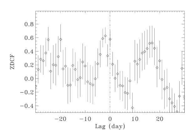
To be more rigorous, we computed the Z-transformed discrete correlation function (ZDCF; Alexander 1997) from light curves in the two bands. The ZDCF makes use of the Fisher’s z-transform of the correlation coefficient (see Alexander 1997 for a detailed description). Its main advantage over the more commonly used DCF (Edelson & Krolik 1988) is that it is more efficient in detecting any correlation present. Figure 6 shows the ZDCF (in 1-day bins) derived from the 2002/2003 data set. The ZDCF seems to peak at a negative lag. Fitting the peak (in the narrow range of -7–7 days) with a Gaussian function, we found its centroid at $-1.8\pm 0.4$ days, which is of marginal significance. If real, the result would imply that the X-ray variability leads the gamma-ray variability. Other ZDCF peaks are most likely caused by the Whipple observing pattern, such as the quasi-periodic occurrences of the dark moon periods. Similarly, we computed a ZDCF for the 2003/2004 data set. The results are shown in Figure 7. In this case, the main feature is very broad and significantly skewed toward positive lags. The feature appears to be a composite of multiple peaks, although large error bars preclude a definitive conclusion. A positive ZDCF peak means that the X-ray emission lags behind the gamma-ray emission. We checked the results with different binning schemes and found no significant changes.

The detection of X-ray lags in the 2003/2004 data set should not come as a total surprise, because we have already seen (from Fig. 2) that the X-ray flux rose more slowly than the gamma-ray flux during the 2004 giant flare. The difference in the rise times can be the cause of the broad ZDCF peak that is skewed toward positive lags. To check that, we excluded the flare from the X-ray and gamma-ray light curves (by removing all data points after MJD 53100; see Fig. 1) and computed a new ZDCF. The results are also shown in Fig. 7 (bottom panel) for a direct comparison. There is a narrow peak at around -1 day. Fitting it (in the range of -7–3 days) with a Gaussian function yields the centroid at $-1.2\pm 0.5$ days, which is not inconsistent the measured value for the 2002/2003 data set though it is even less significant statistically. The features at around +7 and -15 days (which are also discernable in the overall ZDCF) are, again, most likely caused by the Whipple observing pattern for the season. Despite the complications, it is almost certain, by comparing the two ZDCFs, that the X-ray lags in the 2003/2004 data set are indeed associated with the difference between the X-ray and gamma-ray rise times of the giant flare.

To investigate the effects of data gaps (which are present both in the X-ray and gamma-ray data) on ZDCF, we did the following experiment. We created three light curves: the actual X-ray light curve of Mrk 421 in the 2003/2004 season(lc1), an artificial light curve (lc2) made by shifting lc1 by +8 days, and another artificial light curve (lc3) made by modulating lc2 with the Whipple sampling pattern. Figure 8 shows the ZDCFs between lc1 and lc2 and between lc1 and lc3 separately. The artificially-introduced 8-day lag is easily recovered in both cases. We also shifted lc1 by different amounts and the lags are always recovered correctly. Therefore, the coverage gaps associated with the RXTE and Whipple monitoring campaigns do not wash out intrinsic offsets between the X-ray and gamma-ray light curves, although the effects of the data gaps on the shape of the ZDCFs are measurable.

3.1.3 X-ray and TeV Flares

Examining the X-ray and TeV light curves more closely, we noticed that some of the TeV flares have no simultaneous X-ray counterparts (or counterparts at long wavelengths). They are, therefore, similar to the reported “orphan” TeV flare in 1ES1959+650 (Krawczynski et al. 2004). Figure 9 shows an example of the phenomenon. The TeV flare peaks at almost 8 $\gamma\mbox{ }min^{-1}$ at around MJD 53033.4 when the X-ray flux is low. It is interesting to note, however, that the source is clearly variable in X-rays during this time period and that the X-ray flux seems to have peaked about 1.5 days before the TeV flux. Therefore, the TeV flare might not be a true orphan event; it might simply lag behind its X-ray counterpart. Alternatively, it is also possible that the TeV flare is a composite of two sub-flares, with one being the counterpart of the X-ray flare and the other a true, lagging orphan flare. The sparse sampling of the data prevents us from drawing a definitive conclusion in this regard. We note the remarkable similarities between the TeV flare shown in Fig. 9 and the reported “orphan” flare in 1ES1959+650 (see Fig. 4 in Krawczynski et al. 2004), including similar variation patterns in X-rays.

From the X-ray and TeV light curves, we also detected flares on much shorter timescales. Figure 10 shows examples of sub-hour X-ray flares. The most rapid X-ray flare detected lasted only for $\sim$ 20 minutes and shows substantial sub-structures, implying variability on even shorter timescales. Only on one occasion was a sub-hour X-ray flare detected during a (longer-duration) gamma-ray flare. No counterpart is apparent at TeV energies (see Fig. 10), although the error bars on gamma-ray measurements are quite large. We note that, if a strong rapid TeV flare, for example, like the one detected by Gaidos et al. (1995), had occurred, we should have easily detected it, given the improved instrumentation. The rapid X-ray flare shown in Fig. 10 is relatively weak, with a peak-to-peak amplitude of only about 5% of the average flux level. The data do not allow any direct comparison on long timescales, due to the short exposure of the X-ray observation.

3.2 Spectral Energy Distributions

We first divided the RXTE observations into 8 groups based on the X-ray count rate of Mrk 421, with an increment of 20 $cts\mbox{ }s^{-1}\mbox{ }PCU^{-1}$ . For this work, we focused on three of the groups: low (0–20 $cts\mbox{ }s^{-1}\mbox{ }PCU^{-1}$ ), medium (40–60 $cts\mbox{ }s^{-1}\mbox{ }PCU^{-1}$ ), and high (140–160 $cts\mbox{ }s^{-1}\mbox{ }PCU^{-1}$ ), with the average count rate increasing roughly by a factor of three from low to medium and from medium to high. Then, for each observation in a group we searched for an observation at TeV energies that was made within an hour. Only matched pairs were kept for further analysis. We ended up with a total of 16, 9, and 3 pairs in the low-flux, medium-flux, and high-flux group, respectively. It turns out that the low-flux group consists of observations taken between 2003 March 8 and May 3, the medium-flux group between 2004 January 27 and March 26, and the high-flux group between 2004 April 16–20.

For each group, we proceeded to construct a flux-averaged SED at X-ray and TeV energies. The flux-averaged X-ray spectrum can be fitted satisfactorily by a power law with an exponential roll-over (with reduced $\chi^{2}\lesssim 1$ ). We should note that we added a 1% systematic uncertainty to the X-ray data for spectral analysis (which is a common practice), to take into account any residual calibration uncertainty. Also, we fixed the hydrogen column density at $1.38\times 10^{20}\mbox{ }cm^{-2}$ (Dickey & Lockman, 1990). The best-fit photon index is about $2.51^{+0.03}_{-0.05}$ , $2.38^{+0.02}_{-0.02}$ , and $1.99^{+0.02}_{-0.02}$ for the low-, medium-, and high-flux group, respectively, and the roll-over energy about $26^{+3}_{-5}$ , $32^{+3}_{-3}$ , and $32^{+2}_{-2}$ keV. Therefore, the X-ray spectrum of Mrk 421 hardens toward high fluxes. Using the best-fit model we then derived the X-ray SED for each data group.

For the gamma-ray spectral fits, a bin size of 0.1667 in $\log_{10}(E)$ was adopted for the medium- and high-flux groups and a wider bin size of 0.4 for the low-flux group. As shown in Fig. 12, the low-flux SED still has very large error bars. The first energy bin corresponds to an energy of $\sim$ 260 GeV. The gamma-ray spectra can all be satisfactorily fit by a power law, with a photon index of $2.84\pm 0.58$ , $2.71\pm 0.15$ , and $2.60\pm 0.11$ for the low-, medium-, and high-flux groups, respectively. The errors bars only include statistical contributions. For the purpose of comparison with some of the published results, we also fitted the spectra with a cut-off power law (see, e.g., Krennrich et al. 2002) but with the cut-off energy fixed at 4.96 TeV. The photon index is $2.73\pm 0.56$ , $2.40\pm 0.18$ , and $2.11\pm 0.14$ for the low-, medium-, and high-flux groups, respectively. Like the X-ray spectrum, therefore, the TeV spectrum also seems to harden toward high fluxes, although the uncertainty here is quite large.

Finally, we searched for radio and optical observations that fall in one of the groups and computed the average fluxes to complete the SED for the group. Given the fact that Mrk 421 did not vary as significantly at these wavelengths, we believe that the derived SEDs are quite reliable. Figure 12 summarizes the results.

3.3 Spectral Modeling

We experimented with using a one-zone SSC model (see Krawczynski et al. 2004 for a detailed description of the code, which we revised to use the adopted cosmological parameters) to fit the measured flux-averaged SEDs. Briefly, the model calculates the SED of a spherical blob of radius $R$ . The blob moves down the conical jet with a Lorentz factor $\Gamma$ . The emitting region is filled with relativistic electrons with a broken power-law spectral distribution: $S_{e}\propto E^{-p_{1}}$ , for $E_{min}<E<E_{b}$ , and $S_{e}\propto E^{-p_{2}}$ , for $E_{b}\leq E<E_{max}$ (although the code does not evolve the electron spectrum self-consistently). The model accounts for the attenuation of the very-high-energy $\gamma$ -rays by the diffuse infrared background (as modelled by MacMinn & Primack 1996) .

We first found an initial “best fit” to each SED by visual inspections. We then performed a systematic grid search around the “best fit” that involves the following parameters: magnetic field $B$ in the range of 0.045–0.45 G, Doppler factor $\delta$ in 10–20, $p_{1}$ in 1.8–2.2, $p_{2}$ in 2.9–3.7, $log{E_{b}}$ in 9.9–12.2, $log{E_{max}}$ in 9.9–12.2, and the normalization ( $w_{e}$ ) of $S_{e}$ in 0.00675–0.44325 $ergs\mbox{ }cm^{-3}$ . Variability constraints (see the next section) were taken into account in the choice of some of the parameter ranges. All other parameters in the model (e.g., $R$ ) were fixed at the nominal values determined by the visual inspections. We found roughly where the global $\chi^{2}$ minimum lies through a coarse-grid search, and then conducted a finer-grid search through much smaller parameter ranges around the minimum to find the best fit. Figure 11 shows the results for the high-flux group. It is apparent that the model severely underestimates the radio and optical fluxes. Large deviations are also apparent at TeV energies. We should stress that our grid searches are, by no means, exhaustive. However, the results should be adequate for revealing gross discrepancies between the model and the data.

To investigate whether the fit could be improved by introducing additional zones (which are assumed to be independent of each other), we introduced a new zone to account for the radio fluxes and another for the optical fluxes. To be consistent with the observed variability, the additional zones must be placed much further down the jets. Figure 12 shows fits to the SEDs with such a three-zone SSC model. This ad-hoc approach does seem to yield a reasonable fit to the data. In such a scenario, the observed variability at X-ray and TeV energies would be associated with zones close to the central black hole, while radio and optical emission are expected to vary on longer timescales further down the jet.

4 Discussion

4.1 X-ray–TeV Correlation

The success of the standard SSC model lies partly in the fact that it provides a natural explanation for the correlation between the X-ray and gamma-ray emission. However, we found that the correlation is not as tight as one might naively expect from the SSC model. It seems unlikely that the loose correlation is caused by the choice of spectral bands used in the cross-correlation analysis, given how broad the PCA and Whipple passing bands are. In fact, both the derived variability amplitudes (Fig. 4) and SEDs (Fig. 12) indicate that the X-ray and gamma-ray photons are likely to have originated from the same population of electrons in the context of the SSC model.

In the standard SSC model, X-ray photons are Compton upscattered to produce gamma-ray photons, so an X-ray lead is naturally expected. However, the characteristic timescale of the SSC process would be much too short to account for the X-ray lead of 1–2 days (see Fig. 6), although we cannot be sure about whether the lead is actually real, due to large uncertainties and possible systematic effects. What is certain is that the SSC model cannot explain the difference between the X-ray and gamma-ray rise times of the 2004 giant flare. It is conceivable that the flaring episode could have started with an orphan TeV flare and followed by a pair of simultaneous X-ray and TeV flares. If this is the case, it would be opposite to the theoretical scenario recently put forth by Böttcher (2004). In the hadronic models, both X-ray lag and lead could, in principle, occur, even at the same time, depending on the relative roles of the primary and secondary electrons. However, it would also seem challenging for these models to account for the different X-ray and gamma-ray rise times of the 2004 giant flare or to quantitatively explain the long X-ray lead (of 1–2 days) if it is real.

4.2 Variability Constraints

Combined with the measured SED, rapid X-ray flares pose severe constraints on some of the physical properties of the flaring region, in a relatively model-independent manner, because the X-ray emission from Mrk 421 is almost certainly of synchrotron origin. The most rapid X-ray flare detected during our campaign has a duration of about 20 minutes and reaches a peak amplitude of $\sim$ 15% of the (local) non-flaring flux level (see Fig. 10). Therefore, the size of the flaring region must satisfy: $l^{\prime}\lesssim ct_{flare}\delta/(1+z)=3.6\times 10^{14}\delta_{1}\mbox{ }cm$ , where $t_{flare}$ is the duration of the flare ( $=1200$ s), $\delta$ is the Doppler factor of the jet ( $\delta=10\delta_{1}$ ), and $z$ is the redshift of Mrk 421 ( $z=0.031$ ). Here and in the remainder of the paper, we use the primed symbols to denote quantities in the co-moving frame of the jet and unprimed ones corresponding quantities in the frame of the observer. It is interesting to note that the derived upper limit is already comparable to the radius of the last stable orbit around the $2\times 10^{8}M_{\odot}$ black hole in Mrk 421 (Barth et al. 2003), for $\delta\sim 10$ . Since the peak flux of the flare is a significant fraction of the steady-state flux, the size of the flaring region is probably comparable to the lateral extent of the jet (to within an order of magnitude). If the jet originates from accretion flows, as is often thought to be the case, the result would also represent an upper limit on the inner boundary of the flows.

The decaying time of the most rapid X-ray flare (about 600 s) sets a firm upper limit on the synchrotron cooling time of the emitting electrons. The cooling time is given by (Rybicki & Lightman 1979), $\tau^{\prime}_{syn}\approx 6\pi m_{e}c/\sigma_{T}\gamma^{\prime}_{b}B^{\prime 2}$ , where $m_{e}$ is the electron rest mass, $\sigma_{T}$ is the Thomson cross section, $B^{\prime}$ is the strength of the magnetic field in the region, and $\gamma^{\prime}_{b}$ is the characteristic Lorentz factor of those electrons that contribute to the bulk of the observed X-ray emission. By requiring $\tau^{\prime}_{syn}<t_{d}\delta$ , where $t_{d}$ is the measured decaying time of the flare ( $\approx 600s$ ), we derived a lower limit on $B^{\prime}$ , $B^{\prime}>1.1\delta_{1}^{-1/2}{\gamma^{\prime}}_{b,5}^{-1/2}\mbox{ }G$ , where $\gamma^{\prime}_{b}=10^{5}\gamma^{\prime}_{b,5}$ . From modeling the SEDs, we found $2\times 10^{5}\leq\gamma^{\prime}_{b}\leq 4\times 10^{5}$ . It should be noted that the limits derived are only appropriate for the region that produced the 20-min X-ray flare and that not all flares are necessarily associated with the same region. In our attempt to model the SEDs (§ 3.2), we only require that the model parameters be consistent with variability timescales of hours. Results from more sophisticated modeling will be presented elsewhere.

Further constraints can be derived from the detected TeV flares. The fact that we detect TeV photons from Mrk 421 requires that the opacity due to $\gamma\gamma\rightarrow e^{+}e^{-}$ must be sufficiently small near the TeV emitting region(s). This requirement leads to (Dondi & Ghisellini 1995):

\delta\geq\left[\frac{\sigma_{T}d^{2}_{L}}{5hc^{2}}\frac{F(\nu_{t})}{t_{var}}\right]^{1/(4+2\alpha)},

where $d_{L}$ is the luminosity distance, $t_{var}$ is the TeV flux doubling time, $\alpha$ and $F(\nu_{t})$ are the local spectral index and the energy flux, respectively, at the target photon frequency, at which the pair production cross section peaks,

{\nu}{\nu_{t}}\sim\left(\frac{m_{e}c^{2}}{h}\frac{\delta}{1+z}\right)^{2},

where $\nu$ is the frequency of the gamma-ray photon. For $h\nu\sim 1$ TeV, we have $\nu_{t}\sim 6\times 10^{15}$ Hz. From the high-flux SED (Fig. 12), we found $\alpha\sim 0.5$ and $\nu_{t}F_{\nu_{t}}\sim 1\times 10^{-10}\mbox{ }erg\mbox{ }cm^{2}\mbox{ }s^{-1}$ . Given $d_{L}=129.8$ Mpc and $t_{var}\simeq 1$ hour (see Fig. 10), we derived a lower limit on the Doppler factor, $\delta\gtrsim 10$ .

4.3 “Orphan” TeV Flares

Since TeV emission is the consequence of inverse-Compton scattering of (synchrotron) X-ray photons by the electrons themselves in the standard SSC model, a flare at TeV energies must be preceded by an accompanying flare at X-ray energies. While the model might still be able to accommodate the presence of orphan X-ray flares, the presence of orphan TeV flares seems problematic. On the other hand, the “orphan” TeV flares in Mrk 421 (as shown Fig. 9) and in 1ES1959+650 (Krawczynski et al. 2004) might not be orphan events after all. In both cases, the gamma-ray flares seem to be preceded by X-ray flares, which could be attributed to the SSC process although the X-ray lead (of 1–2 days) would seem too long. Alternatively, it might be possible to attribute the X-ray lead to some sort of feedback between different emission regions in the jet (i.e., an orphan X-ray flare in one region triggers an orphan TeV in another).

Genuine orphan TeV flaring would not be easy to understand in the hadronic models either, despite looser coupling between the X-ray and TeV emission, unless the injected e/p ratio changes significantly from flare to flare. Any change in the proton population will likely be accompanied by a change in the electron (primary or secondary) population, so TeV and X-ray flares should both occur as a result. Interestingly, orphan TeV flares may be understood in a hybrid scenario in which protons are present in the jet in substantial quantities but are not necessarily dominant compared to the lepton component (Böttcher 2004). In this case, an orphan TeV flare is associated with (and follows) a pair of simultaneous X-ray and TeV flares that originate in the standard SSC process. The synchrotron (X-ray) photons are then reflected off some external cloud and return to the jet (following a substantial delay with respect to the initial flares). The returned photons interact with the protons in the jet to produce pions and subsequent $\pi^{0}$ decay produces TeV photons in the flare. The model was shown to be able to account for the “orphan” TeV flare observed in 1ES1959+650 (Böttcher 2004). It might also explain some of the similar flares in Mrk 421, for example, the one shown in Fig. 9, if it is a composite of two gamma-ray flares (see discussion in § 3.1.3).

4.4 Spectral Energy Distribution

The SED of Mrk 421 varies greatly both at X-ray and TeV energies but only weakly at radio and optical wavelengths. The much reduced variability at long wavelengths is expected for short timescales, because of long synchrotron cooling times of the radio or optical emitting electrons. In other words, there is no reason to expect a tight correlation between the low-energy (radio or optical) emission and the high-energy (X-ray or TeV) emission. Of course, the lack of such a correlation could also be due to the fact that the low-energy emission originates in regions further down the jet. Between the radio and optical bands, we found that the NVAs of the source are comparable (see Fig. 4), which is somewhat surprising because the synchrotron cooling time of the electrons responsible for the optical emission is expected to be much shorter than that of those for the radio emission. On the other hand, this could be evidence for the presence of different populations of electrons that produce the emission in the radio and optical bands. The populations may be located in physically separated regions and may have different spectral energy distributions (e.g., $E_{max}$ ).

We found that both SED peaks move to higher energies as the luminosity of the source increases. Moreover, the X-ray spectrum becomes flatter, which seems to be common among high-frequency-peaked BL Lacs (e.g., Giommi et al. 1990; Pian et al. 1998; Xue & Cui 2004). Similar spectral hardening has also been see at TeV energies (Krennrich et al. 2002; Aharonian et al. 2002). In our data set, we have seen some indication of spectral hardening but we cannot be certain because of the low statistics of the data. The evolution of the SED could be driven by a hardening in the electron energy distribution and/or an increase in the strength of the magnetic field at high luminosities.

5 Summary

In this paper, we have presented a substantial amount of multi-wavelength data that have been collected on Mrk 421 as the result of a long-term monitoring campaign. The large dynamical range of the data has allowed us to carry out some detailed investigations on variability timescales, cross-band correlation, and spectral variability. The main results from this work are summarize as follows:

•

We have shown that the emission from Mrk 421 varied greatly at both X-ray and gamma-ray energies and that the variabilities in the two energy bands are generally correlated. This is consistent with some of the earlier results but the dynamical range of the data and statistics are much improved here. Equally important is the finding that the correlation is only a fairly loose one (see Figures 5–7). The emission clearly does not always vary in step between the two bands.
•

We have discovered that the X-ray emission reached the peak days after the TeV emission during the giant flare in April 2004 (see Fig. 1). Such a difference in the rise times for the two energy bands poses a serious challenge to the standard SSC model, as well as the hadronic models. Whether it can be accommodated by some hybrid model remains to be seen. In addition, there is tentative evidence that the X-ray variability leads the gamma-ray variability by 1–2 days. If proven real, such a long X-rad lead would also be difficult for either the SSC or hadronic models to explain quantitatively.
•

We have detected X-ray and TeV flares on relatively short timescales. For example, the most rapid X-ray flare detected has the duration of only $\sim$ 20 minutes and a peak amplitude of $\sim$ 15% of the local non-flaring flux level. Although no similarly rapid TeV flares were detected during our campaign, we did observe a TeV flare with duration of hours. Physical constraints on the flaring regions have been derived from the rapid X-ray and TeV variabilities.
•

We have seen TeV flares in Mrk 421 that are similar to the reported “orphan” flare in 1ES1959+650. Genuinely orphan or not, this presents another serious challenge to the proposed emission models (see § 4.3). If they are true orphan events, they may be explained by a hybrid model in which both electrons and protons are present in the jet in substantial quantities. On the other hand, if the preceding X-ray flare turns out to be the counterpart, the 1–2 day X-ray lead would challenge the proposed emission models (see § 3.1.3).
•

We have derived high-quality SEDs of Mrk 421 from simultaneous or nearly simultaneous observations at TeV, X-ray, optical, and radio energies. The X-ray spectrum clearly hardens toward high fluxes; the gamma-ray spectrum also appears to evolve similarly (although we cannot be sure due to large uncertainties of the data). A one-zone SSC model fails badly to fit the measured fluxes at the radio and optical wavelengths, and, to a lesser extent, also underestimates fluxes at the highest TeV energies. The introduction of additional zones improves the fit significantly.
•

Further evidence for the presence of multiple populations of emitting electrons is provided by the comparable radio and optical NVAs (see Fig. 4 and discussion in § 4.4).

We acknowledge the technical assistance of E. Roache and J. Melnick. The VERITAS collaboration is supported by the U.S. Department of Energy, National Science Foundation (NSF), the Smithsonian Institution, NSERC (Canada), PPARC (UK), and Science Foundation Ireland. W. Cui and M. Błażejowski also gratefully acknowledge financial support from NASA and thank Peter Biermann for useful discussions on the subject and comments on the manuscript. UMRAO is supported in part by funds from NSF and from the Department of Astronomy at University of Michigan.

References

(1)
(2) Aharonian, F. 2000, New Astronomy, 5, 377
(3) Aharonian, F., et al. 2002, A&A, 393, 89
(4) Aharonian, F., et al. 2003, A&A, 403, L1
(5) Alexander, T., 1997, in Proc. “Astronomical Time Series”, Eds. D. Maoz, A. Sternberg, & E. M. Leibowitz, (Dordrecht: Kluwer), 163
(6) Aller, H. D., Aller, M. F., Latimer, G. E., & Hodge, P. E. 1985, ApJS, 59, 513
(7) Baars, J.W.M., Genzel, R, Pauliny-Toth, I.I.K., & Witzel, A. 1977, A&A, 61, 99
(8) Beall, J. H., & Bednarek, W. 1999, ApJ, 510, 188
(9) Böttcher, M., et al., 1997, A&A, 324, 395
(10) Böttcher, M. 2002, in Proc. “The Gamma-ray Universe”, XXII Moriond Astrophysics Meeting, eds. A. Goldwurm et al., p. 151
(11) Böttcher, M. 2005, ApJ, 621, 176
(12) Buckley, J. H., et al. 1996, ApJ, 472, L9
(13) Catanese, M., et al. 1997, ApJ, 487, L143
(14) Cui, W. 2004, ApJ, 605, 662
(15) Cui, W., et al. 2004, in Proc. ”International Symposium on High Energy Gamma-Ray Astronomy” (Gamma-2004), eds. F.A. Aharonian and H. Voelk, AIP Conf. Ser., 745, 455 (astro-ph/0410160)
(16) Daniel, M., et al. 2005, ApJ, 621, 181
(17) Dar, A., & Laor, A. 1997, ApJ, 478, L5
(18) Dermer, C. D., et al. 1992, A&A, 256, L27
(19) Dicke, J, & Lockman, J. 1990, ARA&A. 28, 215
(20) Dondi, L., & Ghisellini, G. 1995, MNRAS, 273, 583
(21) Edelson, R. A., & Krolik, J. H. 1988, ApJ, 333, 646
(22) Edelson, R. A., et al. 1996, ApJ, 470, 364
(23) Falcone, A., et al. 2004, ApJ, 613, 710
(24) Finley, J. P., et al. 2001, in Proc. 27th Int. Cosmic Ray Conf., 199
(25) Fossati, G., et al. 1998, MNRAS, 299, 433
(26) Gaidos, J. A., et al. 1996, Nature, 383, 319
(27) Giommi, P., Barr, P., Pollock, A. M. T., Garilli, B., & Maccagni, D. 1990, ApJ, 356, 432
(28) Hillas, A. M., et al. 1998, ApJ, 503, 744
(29) Krawczynski, H., et al. 2004, ApJ, 601, 151
(30) Krennrich. F., et al. 2002, ApJ, 575, L9
(31) LeBohec, S., & Holder, J. 2003, Astropart. Phys., 19, 221
(32) Landolt, A. 1992, AJ, 104, 340
(33) Lyutikov, M. 2003, New Astr. Rev. 47, 513
(34) Mannheim, K., & Biermann, P. L. 1992, A&A, 253, L21
(35) Maraschi, L., Ghisellini, G., & Celotti, A., 1992, ApJ, 397, L5
(36) Maraschi, L., et al. 1999, Astropart. Phys., 11, 189
(37) Marscher, A. P., & Gear, W. K., 1985, ApJ, 298, 11
(38) Mastichiadis, A., & Kirk, J. G., 1997, A&A, 320, 19
(39) MacMinn, D., & Primack, J. R. 1996, Space Sci. Rev., 75, 413
(40) Mochejska, B. J., Stanek, K. Z., Sasselov, D. D., & Szentgyorgyi, A. H. 2002, AJ, 123, 3460
(41) Mohanty, G., et al. 1998, Astropart. Phys., 9, 15
(42) Mücke, A., et al. 2003, Astropart. Phys., 18, 593
(43) Nilsson, K., Pursimo, T., Takalo, L. O., Sillanpää, A., & Pietilä, H. 1999, PASP, 111, 1223
(44) Petry, D., et al., 2000, ApJ, 536, 742
(45) Petry, D., et al., 2002, ApJ, 580, 104
(46) Pian, E., et al. 1998, ApJ, 492, L17
(47) Pohl, M., & Schlickeiser, R. 2000, A&A, 354, 395
(48) Punch, M., et al. 1992, Nature, 358, 477
(49) Rees, M. J., 1978, MNRAS, 184, P61
(50) Reynolds, P., et al. 1993, ApJ, 404, 206
(51) Rybicki, G. B., & Lightman, A. P., Radiative Processes in Astrophysics (New York: John Wiley & Sons)
(52) Sikora, M., et al. 1994, ApJ, 421, 153
(53) Spada, M., et al., 2001, MNRAS, 325, 1559
(54) Stetson, P. B. 1987, PASP, 99, 191
(55) Teräsranta, H., et al. 1998, A&AS, 132, 305
(56) Urry, C. M., & Padovani, P. 1995, PASP, 107, 803
(57) Villata, M., Raiteri, C. M., Lanteri, L., Sobrito, G., & Cavallone, M. 1998, A&AS, 130, 305
(58) Weekes, T. C. 2003, Proc. 28th ICRC (astro-ph/0312179)
(59) Xue, Y., & Cui, W. 2005, ApJ, 622, 160
(60)

Refer to caption — Figure 1: Multiwavelength light curves of Mrk 421. For clarity, the light curves are shown separately for the 2002/2003 (left) and 2003/2004 (right) Whipple observing seasons. For the R-band data, the FLWO points are shown in bullets and the Boltwood points in diamonds. Note that the gamma-ray rates have been corrected for zenith-angle changes, as well as for relative variations in the throughput of the telescope within each season. Also, the differential Boltwood measurements have been scaled up to match the FLWO fluxes (see text). No optical data are available for the 2002/2003 season; the 22 GHz data are shown instead.