X-Ray Emission and Optical Polarization of V1432 Aquilae: An Asynchronous Polar

Abstract

A detailed analysis of X-ray data obtained with $ROSAT$, $ASCA$, $XMM$-$Newton$ and the $Rossi$ $X$-$ray$ $Timing$ $Explorer$ ($RXTE$) for the asynchronous polar V1432 Aquilae is presented. An analysis of Stokes polarimetry data obtained from the South African Astronomical Observatory (SAAO) is also presented. Power spectra from long-baseline $ROSAT$ data show a spin period of 12150 s along with several frequency components related to the source. However, the second harmonic of the spin period dominates the power spectrum in the $XMM$-$Newton$ data. For the optical circular polarization, the dominant period corresponds to half the spin period (or its first harmonic). The $ROSAT$ data can be explained as due to accretion onto two hot spots that are not anti-podal. The variations seen in the optical polarization and the $ASCA$ and $XMM$-$Newton$ X-ray data suggest the presence of at least three accretion foot prints on the surface of the white dwarf. Two spectral models, a multi-temperature plasma model and a photo-ionized plasma model, are used to understand the spectral properties of V1432 Aql. The data from the $RXTE$ Proportional Counter Array (PCA) with its extended high energy response are used to constrain the white dwarf mass to 1.2$\pm$0.1 M_⊙ using a multi-temperature plasma model. The data from the European Photon Imaging Camera (EPIC) on-board $XMM$-$Newton$ are well fitted by both models. A strong soft X-ray excess ($<0.8$ keV) is well modeled by a blackbody component having a temperature of 80–90 eV. The plasma emission lines seen at 6.7 and 7.0 keV are well fitted using the multi-temperature plasma model. However, the fluorescent line at 6.4 keV from cold Fe requires an additional Gaussian component. The multi-temperature plasma model requires two absorbers: one that covers the source homogeneously and another partial absorber covering $\sim 65$% of the source. The photo-ionized plasma model, with a range of column densities for the Fe ions, gives a slightly better overall fit and fits all emission line features. The intensity and spectral modulations due to the rotation of the white dwarf at a period of 12150 s require varying absorber densities and a varying covering fraction of the absorber for the multi-temperature plasma model. The presence of a strong blackbody component, a rotation period of 12150 s, modulation of the Fe fluorescence line flux with 12150 s period, and a very hard X-ray component suggest that V1432 Aql is an unusual polar with X-ray spectral properties similar to that of a soft intermediate polar.

1 Introduction

V1432 Aquilae (RX J1940.1-1025) is an AM Herculis (polar) system in which a white dwarf with a strong magnetic field accretes material from the Roche lobe of a late-type dwarf companion star. It was discovered in the ROSAT PSPC observations of the Seyfert galaxy NGC 6814 (Madejski et al. 1993). Staubert et al. (1994) detected a period of 12120$\pm$3 s in radial velocity of the H_α emission line using optical spectroscopy. The optical photometric and X-ray light curves of V1432 Aql show an eclipse-like structure near orbital phase zero that provided a more accurate orbital period determination. Watson et al. (1995) reported an orbital period of 12116.3$\pm$0.4 s using optical photometry and 12116.3$\pm$0.01 s from combined optical and X-ray dip timings. Further radial velocity measurements by Patterson et al. (1995) and Friedrich et al. (1996) confirmed this period. Watson et al. (1995) argue that the eclipse-like structure is due to absorption in the accretion stream (see also Schmidt & Stockman 2001). Whereas, Patterson et al. (1995) suggest that it is an eclipse by the secondary star. Mukai et al. (2003a) and Singh & Rana (2003) (hereafter Paper 1) argue that this dip is likely a true eclipse by the secondary star based on the absence of any residual X-ray flux at minimum light.

The orbital period of V1432 Aql is well established from the well defined eclipses. The white dwarf spin period (P_spin) is seen in the optical photometry (Patterson et al. 1995) as well as in the X-ray data (Friedrich et al. 1996). Geckeler & Staubert (1997) estimate the white dwarf spin period to be 12150 s from the changing nature of the accretion region relative to the magnetic pole in X-ray ($ROSAT$) and optical photometry. Recently, Staubert et al. (2003) have provided an accurate ephemeris for the spin period using timings of spin minima obtained from the optical photometric and the X-ray data and also detected a secular decrease of 1.013 $\times 10^{-8}$ s/s in the spin period. They estimate a spin period of 12150.328$\pm$0.045 s (for epoch 1995.2) using combined optical and X-ray data. Mukai et al. (2003a) report an analysis of extensive optical photometry and derive an ephemeris of the spin period (12150.432 s) and confirm the presence of its time derivative Ṗ_spin=-9 $\times 10^{-9}$ s/s. Based on these characteristics, V1432 Aql is generally believed to be an asynchronous polar with the unusual characteristic of the spin period being slightly longer than the orbital period. However, Mukai (1998) presented evidence for a spin period of $\sim$4040 s using archival $ROSAT$ data and suggested reclassification of V1432 Aql as an intermediate polar. In paper 1, Singh & Rana supported this conclusion by reporting the strongest peak of the power density spectrum at $\sim$4070 s from the analysis of a continuous observation with $XMM$-$Newton$. Additional characteristics that further distinguish V1432 Aql from other polars are the complex X-ray light-curves and the strong hard X-ray emission (Singh et al. 2003), which are commonly associated with the intermediate polars (IPs).

The accreting material in a polar or an IP forms a strong shock near the surface of the white dwarf that heats the gas to a high temperature ($\sim 10^{8}$ K). The hot plasma in the post-shock region gradually cools and settles on to the surface of the white dwarf, emitting mainly in hard X-rays via thermal bremsstrahlung (Lamb & Masters 1979). Therefore, the post-shock region can be considered to have a continuous temperature distribution, so the use of a multi-temperature plasma model to quantify the temperature distribution is necessary (Done, Osborne & Beardmore 1995). The UV and soft X-ray components (below 2 keV) mainly arise because of the reprocessing of hard X-ray photons from the surface of the white dwarf. The soft X-ray spectral component can be modeled using blackbody emission that is usually dominant in polars. However, recently a few IPs have been observed to show characteristics that are common to both IPs and polars, and these are classified as soft IPs (Haberl & Motch 1995). These systems rotate asynchronously where the binary period is considerably longer than the rotation period of the white dwarf, and their X-ray light curves are strongly modulated at the spin period. In addition to a soft X-ray component they also show polarized optical/IR emission due to electrons in the plasma spiraling in a strong ($\sim 10^{7}$ B) magnetic field, properties similar to that of polars. Phase resolved X-ray spectroscopy of such systems can be particularly useful to learn about the origin of the phase dependent features and the complex absorption effects taking place in the source, and the $XMM$-$Newton$ observatory with its wide energy band and high sensitivity is an excellent instrument to study the spectral nature and its phase-dependent behaviour in polars and IPs. With its moderate energy resolution, $XMM$-$Newton$ can also provide useful information about the Fe line complex. Simultaneous observations in the soft and hard X-ray energy bands provide important information about the energy balance in these systems.

In this paper we present a detailed temporal and spectral analysis of $ROSAT$, $ASCA$, $Rossi$ $X-ray$ $Timing$ $Explorer$ ($RXTE$) and $XMM$-$Newton$ observations from 1992 to 2002. We also present an analysis of Stokes photo-polarimetry obtained at the $South$ $African$ $Astronomical$ $Observatory$ ($SAAO$) in 1994. This paper is organized as follows. In the next section we present the observations and analysis techniques. Section 3 contains results from the timing analysis including the X-ray and the circular polarization power spectra and spin folded X-ray light curves. Section 4 contains the results of the spectral analysis and a description of spectral models that are used to characterize the source. The results of the phase resolved spectroscopy are presented in §5. In §6, we discuss the timing and the spectral results, and compare them with other polars and IPs. We conclude and summarize the results in §7.

2 Observations & Data Analysis

2.1 $ROSAT$

V1432 Aql was observed serendipitously with the $ROSAT$ (Trümper 1983) Position Sensitive Proportional Counter (PSPC) in 1992–1993 during the observations of a nearby Seyfert galaxy NGC 6814. Data from these observations were previously analyzed for temporal analysis by Staubert et al. (1994), Friedrich et al. (1996), Mukai (1998), and Staubert et al. (2003). During the 1992 October observations, most of the data were collected in last four days, hence for generating power spectra the data from only the last four days have been used (i.e. 1992 October 27–30) (see Mukai 1998). The 1993 October observations were made at different offset (17$\arcmin$) than the other two (37$\arcmin$). We have made no attempt to account for the different offsets because the light curves are folded separately and this will only affect the average intensity of the source and not the overall profile of the intensity modulation and the intrinsic variability of the source. We extracted the background subtracted source light curves in three energy bands of 0.1–0.5 keV (soft), 0.5–2 keV (medium) and 0.1–2 keV (total) with a time resolution of 4 s, from a circle with a radius of $2\arcmin$.5 centered on the peak position. We used the XSELECT program in FTOOLS (see http://heasarc.gsfc.nasa.gov/docs/software.html) and performed a detailed temporal analysis, exploiting the long baseline of the $ROSAT$ observations.

2.2 $ASCA$

The $ASCA$ observatory (Tanaka, Inoue, & Holt 1994) observed V1432 Aql serendipitously during 1997 October 27–29 while observing a high redshift quasar, PKS 1937-101. Here we have reanalyzed the Gas Imaging Spectrometer (GIS2; Ohashi et al. 1996; Makishima et al. 1996) ‘PH’ mode data with a time resolution of 16 s using the standard screening criteria. For further details the reader is referred to Mukai et al. (2003a). The light curves were extracted in two energy bands of 0.7–2 keV (medium) and 2–10 keV (hard) to facilitate a direct comparison with the light curves obtained from the $ROSAT$ and the $XMM$ observations.

2.3 $XMM$-$Newton$

The $XMM$-$Newton$ observatory (Jansen et al. 2001) observed V1432 Aql continuously on 2001 October 9 for 25455 s with the European Photon Imaging Camera (EPIC) containing two MOS CCDs (Turner et al. 2001). The data from the EPIC PN camera were not available in the observing mode used and the counts in the Reflection Grating Spectrometers (RGS1 and RGS2; den Herder et al. 2001) were insufficient for a meaningful spectral analysis. We adopted an energy range of 0.2–10 keV (a background flare affects the data above 10 keV) for the light curve and time-averaged spectral analysis. X-ray spectra and light curves were extracted for MOS1 and MOS2. We use the $rmfgen$ and $arfgen$ SAS (Science Analysis System ver. 5.4.1) tasks to generate the appropriate response files for both MOS cameras. Individual spectra were binned to a minimum of 20 counts per bin to facilitate the use of $\chi^{2}$ minimization during the spectral fitting. X-ray light curves were extracted in 4 energy bands; soft (0.2–0.5 keV), medium (0.5–2.0 keV), hard (2–10 keV), and total (0.2–10 keV) such that the soft and medium bands correspond roughly to the $ROSAT$ soft and medium bands, respectively. $XMM$-$Newton$ light curves were presented in Figure 1 of Paper 1.

2.4 $RXTE$

V1432 Aql was observed twice with the $RXTE$ Proportional Counter Array (PCA; Jahoda et al. 1996) during 2002 July 14–15 (PI: P. Barrett). The observations were done at an offset of $\sim$15$\arcmin$ from the source to minimize the contamination from the Seyfert galaxy NGC 6814 which is $\sim 37\arcmin$ away. At this offset the contamination from NGC 6814 is $\sim 10$%. The data were processed using the FTOOLS version 5.2 following the standard procedure. We analyzed the PCA standard 2 data with a time resolution of 16 s. For an improved signal-to-noise ratio, data in the 2–10 keV energy band from top xenon layer of all proportional counter units (PCUs) were used to generate the source and the background light curves and spectra. The background light curve and spectrum were obtained using the appropriate background model corresponding to the epoch of each observations. Only three of the five PCUs were ON during the two observations. However, data from PCU0 were rejected, because a propane leak resulted in a large background flare affecting the top layer data from PCU0. Data from only 2 PCUs which are free from the background flare, were analyzed.

2.5 Stokes Polarimetry

Stokes (simultaneous linear and circular) polarimetry data of V1432 Aql were obtained using the University of Cape Town (UCT) polarimeter (Cropper 1985) on the 1 m telescope of the SAAO during 1994 July 5, 6, 8, and 10–13. Most of the data were taken in white light (no filter), though there were short periods of data taken with the B, V, Cousins R, Cousins I, and an extended red (OG570) filters. The integration time was 10 s for the photometry and $\sim$5 minutes for the polarimetry. The UBVRI filters were calibrated before each run using standard stars and the waveplate offset angles were calibrated using linear polarization standard stars. Background exposures were taken at regular intervals to determine the net flux and polarization.

3 Timing Analysis

The three $ROSAT$ observations during 1992–1993 with a mean separation of about six months, provide sufficient frequency resolution to search for fundamental periods, their harmonics and side-bands. The frequency resolution from the combined $ROSAT$ data is $8.13\times 10^{-9}$ s^-1 and that from the $XMM$-$Newton$ data it is $9.83\times 10^{-6}$ s^-1. However, the $XMM$ data continuously span two complete binary orbits, while those of $ROSAT$ data have gaps due to Earth occultation, SAA passage and frequent switching of targets. These gaps lead to complications in the power spectrum as the true variations in the source are further modulated by the irregular sampling defined by the window function of the data. We have used four methods to search for the periodicity present in the $ROSAT$ data: the discrete Fourier transform, the Lomb-Scargle periodogram (Horne & Baliunas 1986), the Bayesian statistical approach (Rana et al. 2004) and the one-dimensional “CLEAN” algorithm (Roberts, Lehar, & Dreher 1987) as implemented in the PERIOD program (ver. 5.0-2) available in the STARLINK package. The Bayesian approach is mathematically more rigorous and can provide optimum number of frequencies allowed by the data independent of the shape of the periodic signal. In the CLEAN algorithm, the discrete Fourier transform first calculated from the light curve is followed by the deconvolution of the “window” function from the data. Here the power is defined as the square of the half amplitude at the specified frequency. This method has been demonstrated to work effectively for X-ray data from various satellites (Norton et al. 1992a, 1992b; Rana et al. 2004). We applied the barycentric correction to all the data sets before carrying out the power spectral analysis. In addition, the data were detrended by subtracting a mean count rate prior to generating power spectra using above methods.

3.1 Power Spectra

3.1.1 $ROSAT$ PSPC

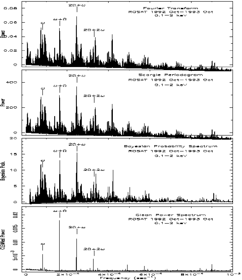
The power spectra obtained using above mentioned methods for the combined $ROSAT$ data in the 0.1–2 keV energy band, are shown plotted in the Figure 1. All power spectra show four common significant peaks related to one of the fundamental period and various side bands of the two fundamental periods of the system, as marked in the figure. The two fundamental frequencies of the system are referred to as $\omega$, corresponding to the presumed spin period and $\Omega$ corresponding to the orbital period. The power spectra presented in first three panels of Fig. 1 show equally prominent peaks at the two fundamental periods, suggesting that a combination of orbital and spin modulations are at work in V1432 Aql. However, a significant peak is seen at a frequency of 12150.72$\pm$1.14 s in CLEAN power spectrum, which is consistent with the $\omega$ that is reported by Mukai et al. (2003a) and Staubert et al. (2003). No significant power is observed at $\Omega$, which has a period of 12116.2824$\pm$0.0043 s (Mukai et al. 2003a), suggesting that the data are modulated primarily on spin period. The other dominant peaks in the power spectra correspond to the $\Omega$+$\omega$, 2$\Omega$+$\omega$, and 2$\Omega$+2$\omega$ components.

In order to study the variations in the power density spectrum with energy, we also calculated the power spectra for the soft and medium energy bands (see §2.1). The power spectra for the soft X-ray energy band show a dominant peak at the 2$\Omega$+$\omega$ component. The second dominant peak, with almost equal power to that of first one, corresponds to the 2$\omega$ component, the first harmonic of the spin period. Prominent peak is also seen at $3\Omega+3\omega$ component. The power spectra for the medium energy X-ray band show a dominant peak at the 2$\omega$-$\Omega$ component. The other dominant peaks correspond to frequency components 2$\Omega$+2$\omega$, 2$\omega$+$\Omega$, $\Omega$+$\omega$, and $\omega$ in order of decreasing power.

3.1.2 $XMM$-$Newton$ MOS

Discrete Fourier transforms are performed on the X-ray light curves with 1 s time resolution. The power spectra in the various energy bands of the $XMM$-$Newton$ data were published in Paper 1. However, the peaks in the power spectra need to be reassigned based on the spin and orbital periods being 12150.432 s and 12116.2824 s (Mukai et al. 2003a), respectively. The power spectrum obtained from averaged MOS1 and MOS2 data in the energy range of 0.2–2 keV is shown plotted in Figure  2. The energy range is chosen so that this power spectrum can be directly compared with that of $ROSAT$ total energy band. However, the shorter baseline gives broader peaks in the power spectrum and several frequency components are indistinguishable. For example, the two fundamental frequencies $\omega$ and $\Omega$ have their power merged in to a single peak. In addition, several harmonics and side band frequencies of the fundamental periods are merged together, they are 2$\omega$ and $\Omega$+$\omega$; 3$\omega$, 3$\Omega$, $\Omega$+2$\omega$ and 2$\Omega$+$\omega$; 4$\omega$, 4$\Omega$, $\Omega$+3$\omega$ and 3$\Omega$+$\omega$; and 9$\omega$ and 9$\Omega$ as shown in Figure 2.

3.1.3 Circular Polarization in the Optical

The polarization data are noisier as compared to the X-ray data and suffer from poor and uneven sampling. As a result the CLEAN procedure is not as effective here as for X-ray data, and when used to generate the power density spectrum from the polarization data, produces several strong peaks at unexplained periods. The power in the unidentified peaks dominates over peaks at true system related periods. Therefore, only a discrete Fourier transform is presented (Figure 3) for the circular polarization data. The most dominant peak in the power spectrum corresponds to a 1 day positive alias of the 2$\omega$ component and is marked as $A^{+}_{2\omega}$. Several peaks can be seen coincident with the fundamental frequency $\omega$ and its various harmonics i.e. 2$\omega$, 3$\omega$, 4$\omega$ and 5$\omega$. Power in the peak at the 5$\omega$ component is higher than at 3$\omega$ and 4$\omega$. Several other unidentified peaks with significant power, are also present in the power spectrum.

3.2 Spin Folded X-ray Light curves

To study variations in the X-ray intensity of the source as a function of spin phase, we have folded the X-ray light curves on the spin period of the system. The X-ray light curves folded with the orbital period are already studied in previous publications (see Mukai et al. 2003a and Paper 1). When folding the X-ray data we have tried two spin ephemerides as given by Mukai et al. (2003a) and Staubert et al. (2003), including the effect of $\dot{P}$. We find that the spin ephemeris as given by Mukai et al. (2003a) better defines the spin minima for the X-ray data from recent years (after 1997), and that of Staubert et al. (2003) is well suited for the data from the earlier years (before 1997). Since Mukai et al. (2003a) obtained the spin ephemeris using the optical data spanning 7 years of base line with clustering around 1998, that could be the reason for its better fit to the spin minima for the data from the $ASCA$, $XMM$-$Newton$ and $RXTE$. On the other hand, Staubert et al. (2003) have used optical and X-ray data taken during 1992–1997 to calculate the spin ephemeris, and that could account for a better definition of the spin minima for the $ROSAT$ data. With respect to a reference zero point defined using Mukai’s ephemeris, the spin folded features obtained using Staubert’s ephemeris show a varying phase shift from a negative value of -0.13 during 1992 October to a positive value of +0.1 during 2002 July. Spin folded light curves in the three energy bands of soft, medium and hard X-rays are presented in Figures 4, 5 and 6, respectively. Their main features are described below.

3.2.1 Soft X-rays

Spin folded soft X-ray light curves for the three $ROSAT$ observations in the 0.1–0.5 keV energy band (first three panels) and for the $XMM$-$Newton$ observation in the 0.2–0.5 keV energy band (bottom panel) are shown in Figure 4. The light curves during 1992 October and 1993 March show similar profiles with a double hump structure and a low intensity state during the 0.3–0.7 phase. The prominent humps span a phase range of 0.7–0.95 during 1992 October, and 0.7–0.9 during 1993 March. The secondary humps (with smaller amplitude) are of similar width as that of the primary but show a small phase shift during the two observations. The broad dip around the phase zero contains two small peaks during 1992 October and is flat and relatively narrower during 1993 March. The light curve for the 1993 October observation (third panel) is highly variable showing three narrow prominent peaks around phases 0.2, 0.75, and 0.88 and a low intensity state during the $\sim$0.25–0.7 phase range with a small flat bottomed dip around phase 0.37. There is a broad dip between the phase range $\sim$0.95–1.12 that is split into two small dips by an interpulse at phase 1.08. For the $XMM$-$Newton$ data, the profile based on ephemeris from Mukai et al. (2003a) (solid line) shows a systematic shift of phase $\sim$0.1 with respect to the profile based on ephemeris from Staubert et al. (2003) (dash-dotted line). The folded light curves show three peaks and three dips as opposed to the double hump profile of the $ROSAT$ light curves of 1992 October and 1993 March, but similar to the $ROSAT$ 1993 October light curves, albeit, with different widths and locations for the humps. The three minima are at phases 0.35, 0.65, and 1.05, respectively. The width of the minimum increases with the increasing spin phase. The minimum at 0.65 is flat bottomed with a very sharp drop and a slow rise of the intensity, whereas the other two minima have roughly the same falling and rising times. The third minimum at phase 1.05 is completely flat bottomed with a constant intensity during 0.95–1.15.

3.2.2 Medium Energy X-rays

The spin folded light curves in the 0.5–2 keV energy band for $ROSAT$, $XMM$-$Newton$, and in the 0.7–2 keV energy band for the $ASCA$ observations are shown plotted in Figure 5. The two different line styles represent folded profiles for the same two ephemerides as used in Fig. 4. The X-ray light curves in the first two $ROSAT$ observations show broadly similar features with a double hump profile. The width of the prominent humps are identical but show a small phase shift during the 1992 October and 1993 March observations, respectively, while the broader asymmetric peaks cover phase ranges of $\sim$0.6–0.95 and $\sim$0.6–0.9. The intensity of the source is low but highly structured during the phase range $\sim$0.3–0.6. The spin profile during the third $ROSAT$ observation is highly variable showing several peaks and dips unlike in the first two observations. The maximum of a prominent peak at phase 0.88 coincides with the broad asymmetric peaks in the first two panels. A second peak near phase 0.2 resembles a peak during the 1992 October light curve but with a relatively low amplitude. The low intensity phase of the source is narrower and not as flat as that shown in the first two panels. The broad dip around phase zero is quite similar to that observed during 1992 October with the presence of an interpulse at phase 1.08. The $ASCA$ light curve shows three humps – one at phase 0.15 and two with relatively lower amplitudes at phases 0.45 and 0.7, respectively. The folded light curve obtained from the $XMM$-$Newton$ data also shows three humps, with an increasing amplitude with increasing spin phase. The dip at phase 0.35 is narrower and shallower than the dip at 0.65. During the broadest dip around 1.05 the intensity is not completely flat, instead shows a slow rise. The peak at phase $\sim$0.45 coincides with that observed in the $ASCA$ light curve, whereas the other two peaks show a small phase shift.

Although overall profiles of the medium and soft energy band light curves are roughly similar, the width and the amplitude of the peaks and dips are different. For the first two $ROSAT$ observations, the secondary peak in the soft X-ray light curves becomes more prominent in the 0.5–2 keV band while the widths remain unchanged; however the primary peak becomes broader and asymmetric. On the other hand, during the 1993 March observations, both the width of the peaks and their relative intensity are different in the two bands. Similarly, for the $XMM$-$Newton$ observations, the relative amplitudes of the peaks in the medium energy band are different than in the soft X-ray band but the widths of the peaks remain almost the same. The power spectra and light curves in different energy bands show that the $ROSAT$ data are primarily modulated on the spin period, confirming the claim by Staubert et al. (2003). On the other hand, Mukai et al. (2003) reported that the hard X-ray $BeppoSAX$ data are modulated on the orbital period.

3.2.3 Hard X-rays

Figure 6 shows the folded profiles in the 2–10 keV energy band for the $ASCA$, the $XMM$-$Newton$ and the $RXTE$ observations, using the spin ephemeris as given by Mukai et al. (2003a). The $ASCA$ light curve shows three humps separated by three dips with the humps located at similar phases as in the medium energy band. The $XMM$-$Newton$ light curve, has a profile that is broadly similar to that in the other two energy bands (Fig. 4 & 5); the only significant difference being in the shape of the minimum at phase 0.65. In hard X-rays, it is very sharp and narrow, suggesting a rapid uncovering of the hard X-ray source, while the softer X-ray source remains covered. Because of the insufficient exposure time, the $RXTE$ data could not cover the entire spin cycle and there are gaps in the folded light curve. The $RXTE$ light curve shows a broad peak during phase 0.6–0.75 followed by a sharp drop ($\sim$17 times) in the intensity. This low intensity phase continues at least up to the 0.93 spin phase. Two more peaks are seen near phases 0.12 and 0.22, the second of these coinciding with the peak observed in the $XMM$-$Newton$ light curve. Both the $XMM$-$Newton$ and the $RXTE$ hard X-ray profiles show two dips at spin phases $\sim$0.17 and $\sim$0.35, respectively.

3.3 Spin Folded Optical Polarization Curves

Figure 7 represents the optical Stokes polarimetry data folded on the spin period using the ephemeris as given by Staubert et al. (2003). We have combined the data from all nights to produced the average binned polarization curves, since the individual unbinned polarization light curves show almost the same trends. The linear polarization shows a broad peak covering a phase range of $\sim$0.45–0.80 that is suddenly cut by a narrow dip around phase 0.6. The position angle remains almost constant over a phase interval of 0.0–0.4 with an average value of $\sim$104^∘. It shows a broad asymmetric dip during phase 0.4–1.0 with a fast decline to a minimum value of 50^∘ and a slow rise to a maximum value of $\sim$140^∘. The circular polarization data shows modulation over the spin period with two peaks – a narrow peak around phase 0.1 and a broad peak around phase 0.6. Both positive and negative values ranging from -1% to 2% are seen.

4 X-ray Spectral Analysis

The time-averaged X-ray spectra obtained from the $RXTE$ and the $XMM$-$Newton$ observations are shown in Figures 8, 9 & 10. The overall shape of the spectra obtained from the two $RXTE$ observations is quite similar except that the normalized intensity is slightly lower during 2002 July 15. The $RXTE$ spectra are very hard and extend to $\sim$30 keV. They also show a broad emission feature between 6 and 7 keV. The $XMM$-$Newton$ spectra show the presence of three emission lines at 6.4, 6.7, and 7.0 keV, with the first line being the strongest. Strong soft X-ray emission is also present in the $XMM$-$Newton$ spectra.

Various plasma models have been used to describe the X-ray spectra of the magnetic CVs (MCVs). These include thermal bremsstrahlung, MEKAL (Mewe et al. 1985; Liedahl et al. 1995), CEVMKL, and cooling flows as given in XSPEC. The MEKAL plasma code describes X-ray emission lines from several elements and continuum expected from hot optically thin plasma assuming a single temperature for the X-ray emitting plasma. The CEVMKL is a multi-temperature version of the MEKAL code with the emission measure defined as a power law in temperature (Singh et al. 1996). The models include line emission from elements like He, C, N, O, Ne, Na, Mg, Al, Si, S, Ar, Ca, Fe, and Ni. None of these models is a true representation of the physical conditions that exist in the X-ray emission regions of the MCVs. Spectral models, which can better describe the physical conditions in MCVs, are the multi-temperature plasma model (model A) as described by Cropper et al. (1999), and the photo-ionized plasma model (model B) as described by Kinkhabwala et al. (2003). Ramsay et al. (2004a) have used model A to analyze the spectra of three polars that were observed by the $XMM$-$Newton$ EPIC detectors (see the references therein for the use of this model to other polar systems). Similarly, Mukai et al. (2003b) have used model B to describe the high resolution spectra of three IPs obtained with the High Energy Transmission Grating (HETG) on-board the $Chandra$ observatory. In this paper, we apply model A to the $RXTE$ spectra, and models A and B to the $XMM$-$Newton$ MOS spectra.

4.1 Multi-temperature Plasma Model

The details about the formulation and the assumptions used in the multi-temperature plasma model are described in Cropper et al. (1999). The model was obtained via private communication from G. Ramsay in 2003. The model predicts the temperature and the density profile of a magnetically confined hot plasma in the post-shock region based on the calculations of Aizu (1973). It uses the ‘MEKAL’ plasma code available in XSPEC to describe the continuum and the line emission from a collisionally ionized hot plasma. Additionally, it takes into account the cyclotron cooling effects that are important for MCVs. The model includes the reflection of hard X-rays from the white dwarf surface and the effects of the gravitational potential on the structure of the post-shock region assuming a stratified accretion column and a one-dimensional accretion flow. The model uses the mass-radius relationship of Nauenberg (1972) to estimate the mass of the white dwarf. It has a total of 8 free parameters. They are the ratio of time scales of the cyclotron cooling to the bremsstrahlung cooling ($\epsilon_{0}$), the specific accretion rate ($\dot{m}$), the radius of the accretion column ($r_{c}$), the mass of the white dwarf ($m_{1}$), the Fe abundance relative to solar, the number of vertical grids in which the shocked region is divided, the viewing angle to the reflecting site, and the normalization. To minimize the number of free parameters, some of the system-dependent parameters are held constant. In this analysis, the viewing angle is fixed to $75^{\circ}$ and the post-shock region is divided into 100 vertical layers. Changing the value of viewing angle over a wide range does not significantly affect the spectral fit. By allowing the remaining parameters to vary, the best fit was found when $\epsilon_{0}\simeq$0.001, which is suitable for low field systems (Wu, Chanmugam and Shaviv 1994) including IPs (Cropper et al. 1998). It is difficult to estimate the magnetic field of the white dwarf in V1432 Aql owing to the poor quality of optical polarization data and lack of cyclotron spectra. Considering the analogy with another polar VV Pup and assuming that the peak in circular polarization of V1432 Aql corresponds to the sixth to eighth harmonic of the cyclotron line, the magnetic field can have a value in the range of 28–35 MG. However, fixing $\epsilon_{0}$ to a higher value also provides an equally good fit to the MOS spectra, and the spectral fit is hardly sensitive to change in $\epsilon_{0}$. The radius of the accretion column is fixed to $10^{8}$ cm, close to its best fit value. The specific accretion rate ($\dot{m}$) is also fixed to 1 g cm^-2 s^-1, which is characteristic of an intermediate accretion state.

Neutral absorbers with a full or partial covering of the source are used to account for the intrinsic absorption seen in the spectra using the phabs model of XSPEC and the H and He absorption cross-sections of Balucinska-Church & McCammon (1992) and Yan et al. (1998), respectively. The multi-temperature plasma model and a partial covering absorption component along with an absorption due to interstellar matter (ISM) and a Gaussian line (phabs$\times$pcfabs(sacg+gaussian)) are used to fit the time-averaged $RXTE$ spectra of V1432 Aql. The two $RXTE$ spectra are fitted simultaneously, since the spectral parameters from individual fits are not significantly different. The different intensities of the two spectra are accounted for by different normalization constants. The multi-temperature plasma model does not predict the fluorescent emission from cold Fe at 6.4 keV, although it does predict the emission lines at 6.7 and 7.0 keV from highly ionized Fe. A Gaussian line model centered at 6.4 keV with an assumed width of 0.1 keV is, therefore, added to fit the $RXTE$ spectra, and a reduced $\chi^{2}_{min}$ of 1.23 for 106 degrees of freedom (dof) is obtained. The best fit value for the column density of the partially covering absorber is $N_{H}\simeq 28^{+5}_{-8}\times 10^{22}$ cm^-2 with a covering fraction of $55^{+5}_{-7}$%. The best fit value for the mass of the white dwarf is found to be $1.21\pm 0.10$ M_⊙. Simultaneous fits to both the spectra along with the best fit model are shown plotted in Figure 8 (top). The bottom panel shows the ratio of the data to the best fit model. Based on these results the mass of the white dwarf is fixed at 1.21 M_⊙ for the spectral analyses of the $XMM$-$Newton$ data.

Since the $XMM$-$Newton$ data extend down to 0.2 keV, additional components such as a blackbody, absorption due to the interstellar matter (ISM), and an additional absorber fully covering the source are needed to fit and to characterize the spectra. The value of interstellar absorption along the direction of V1432 Aql (distance=230 pc; Watson et al. 1995) is fixed as follows: the ISM hydrogen column density search tool from the EUVE Web site is used to estimate the column density in a given direction. (Refer to Fruscione et al. 1994 for the details of the database and the different methods used by this tool to estimate the column density in a given direction.) For the 10 nearest neighboring sources at distances ranging from 130 to 280 pc, the estimated column density varies over a large range from $10^{19}$ to $1.6\times 10^{21}$ cm^-2. Schmidt & Stockman (2001) measured a visual extinction A_v=0.7$\pm$0.1 mag from the interstellar absorption features using Hubble Space Telescope ($HST$) UV spectrum for V1432 Aql. The corresponding neutral hydrogen column density estimated by them is $N_{H}\sim 1.3\times 10^{21}$ cm^-2. $XMM$-$Newton$ spectra gave a poor value for the reduced $\chi^{2}$ (1.6 for 736 dof) with the $N_{H}$ fixed at this value. An independent measurement for the hydrogen column density provided by the $ROSAT$ data (Staubert et al. 1994), gives a value of $6.7^{+3.3}_{-2.2}\times 10^{20}$ cm^-2. With the value of $N_{H}$ fixed at the best fit value of the $ROSAT$ measurement and the two extreme point values (68% joint confidence limits for three parameters), the $XMM$-$Newton$ data prefer to have the lowest value for the $N_{H}$ owing to the ISM. The lowest allowed value of $N_{H}$ from $ROSAT$ data can better describe the $XMM$-$Newton$ data with $\Delta\chi^{2}\sim$180 as compared to the $HST$ measurement. Since the range of $N_{H}$ due to the interstellar absorption obtained from the EUVE database is very large, (with the $ROSAT$ measured value well within the range), and the data indicate the lowest value, a value of $4.5\times 10^{20}$ cm^-2 is adopted for all spectral analysis.

The two MOS data sets are initially fitted separately with a model consisting of a blackbody component, an ISM component, a partial covering absorber, and a multi-temperature plasma component, along with a Gaussian line centered at 6.4 keV to account for the Fe fluorescent emission (phabs(bbody+pcfabs(sacg+gaussian))). In order to fix the value of the line width in the Gaussian, the width is stepped over a range of 0.01–0.2 keV. Values of the line width $>0.1$ keV begin to merge the line with the continuum without significantly affecting the fit and the spectral parameters. Whereas, line widths $<0.05$ keV are narrower than observed. Therefore, we fix the fluorescent line width at 0.05 keV. The spectral parameters derived from individual fits to two MOS spectra are found to have similar values. Therefore, in subsequent analyses simultaneous fits to both MOS spectra are done to improve the statistics. This model gives a reduced $\chi^{2}_{min}$ of 1.5 for 737 dof and the best fit values for the interesting spectral parameters are: a blackbody temperature kT${}_{bb}\simeq 73\pm 2$ eV, a partial covering absorption density, $N_{H}$=$(8.0\pm 1.0)\times 10^{22}$ cm^-2 with a covering fraction of $\sim 68\pm 1$%, and a Fe abundance of $0.83^{+0.17}_{-0.20}$ relative to solar. The quoted error bars (here and in rest of the paper) are for a 90% confidence limit for a single parameter (i.e. $\Delta\chi^{2}$=2.71). The addition of an extra absorber completely covering the source significantly improves the fit by decreasing the reduced $\chi^{2}_{min}$ to 1.35 for 736 dof (phabs(bbody+phabs$\times$pcfabs(sacg+gaussian))). This model gives best fit values of 88$\pm$2 eV for the blackbody temperature, $N_{H1}$=1.7$\pm$0.3 $\times 10^{21}$ cm^-2 for the additional absorber, and $N_{H2}$=$13.0^{+2.0}_{-1.0}\times 10^{22}$ cm^-2 for a partial absorber covering $\sim 65\pm 1$% of the source. The Fe abundance is 0.70$\pm$0.15 relative to solar (Anders & Grevesse 1989). The best fit values of the spectral parameters obtained using the multi-temperature plasma model are listed in Table 2. The jointly fitted MOS spectra with the best fit model are shown in Figure 9 along with the contributions from the individual model components. The ratio of the data to the best fit model are also shown to indicate the quality of the fit. The inset of the figure shows an enlarged view of the 6.0 to 7.5 keV energy range which contains the fluorescent line and the He-like and H-like Fe K_α lines at 6.4, 6.7, and 6.95 keV, respectively.

The need for a strong blackbody component is checked by fitting the MOS spectra using only absorbed multi-temperature plasma model and the Gaussian line, but without the blackbody component. The fit is unacceptable with a reduced $\chi^{2}_{min}$ of $\sim$8 for 738 dof. The residuals in terms of the ratio of the data to the model are shown in Figure 11 (top). The ratio plot shows a strong soft X-ray excess below 0.8 keV which is well represented by a blackbody component as shown in Fig. 9.

The line parameters of three Fe K_α lines are determined by fitting a simple bremsstrahlung model along with three Gaussians in the energy range of 5–9 keV. The continuum around the line region is first evaluated by fitting a bremsstrahlung model and ignoring the 6.0–7.2 keV energy range containing the three lines. Then, the ignored energy range for the lines is retrieved and fitted with the three Gaussians. The width of each Gaussian is kept fixed at 0.05 keV. The reduced $\chi^{2}_{min}$ is 1.05 for 243 dof. This method gives the best fit values for the fluorescent, He-like and H-like line energies as, $6.43^{+0.03}_{-0.02}$, $6.70^{+0.03}_{-0.04}$, and $7.00^{+0.04}_{-0.03}$ keV, respectively; and the line intensities as, 3.84 $\times 10^{-5}$, 3.07 $\times 10^{-5}$, and 2.55 $\times 10^{-5}$ photons cm^-2 s^-1, respectively.

4.2 Photo-ionized Plasma Model

The spectral model of Kinkhabwala et al. (2003) describes the X-ray spectroscopic features expected from a steady-state, low-density photo-ionized plasma and is used as an alternative model to the multi-temperature plasma model. The model has a simple geometry consisting of a cone of ions irradiated by a point source located at the tip of the cone. The line emission is assumed to be unabsorbed and all lines are assumed to be unsaturated at all column densities. This model is available as a local model ‘PHOTOION’ for XSPEC. The assumption of unsaturated lines corresponds to the value of 7 for parameter 1 in the model and is particularly suitable for use with spectra of CVs (see Mukai et al. 2003b). This model contains a large number of free parameters including a power law continuum, some system dependent parameters, and the ionic column densities for various elements. Some of the system dependent parameters are held constant. The covering fraction, defined as $f$=$\Omega$/4$\pi$ for a cone geometry, is set at 0.5, since half of the X-ray flux impinges on the white dwarf surface and the other half is radiated toward the observer. The quantity $\Omega$ is the solid angle subtended by the plasma. The radial velocity width $\sigma$ is held fixed to its default value of 100 km s^-1. The total power law luminosity is defined as L(E)=AE^-Γ, where A is the normalization of the continuum and $\Gamma$ is the power law index. The distance to the source is fixed at 230 pc (Watson et al. 1995).

The MOS spectra are first fitted using the photo-ionized plasma model along with ISM absorption in the energy range 0.8–10 keV, excluding the blackbody dominated soft X-ray energy range ((phabs$\times$photoion)). The ISM column density is kept fixed at 4.5 $\times 10^{20}$ cm^-2 (see §4.1). The individual ionic column densities are not well determined owing to the moderate energy resolution. We therefore set them to their default values of 0.0, except for the column densities of the Fe ions. The column densities of the 26 Fe ionization states are varied one-by-one to find values that reproduce the line emission in the 6–7 keV range, as well as the low energy ($<2$ keV) continuum. This exercise shows that several ions can be grouped together to explain the Fe K-shell and L-shell emission. The H-like and He-like Fe K_α lines at 7.0 and 6.7 keV are respectively fitted with column densities of $3\times 10^{18}$ and $2\times 10^{18}$ cm^-2. As mentioned in §3.1, the 6.4 keV fluorescent line shows a measurable intrinsic width and can not be estimated by varying the neutral Fe column density alone. It is, therefore, necessary to adjust the column densities of the remaining Fe ions (Fe I–XXIV) in three different groups: Fe I–XVI, Fe XVII–XIX, and Fe XX–XXIV with the estimated column densities of $8\times 10^{18}$ cm^-2, $3\times 10^{18}$ cm^-2, and $3\times 10^{17}$ cm^-2, respectively, for a good fit to the data. With the ionic column densities for Fe fixed, the best fit value of the power law index is $\Gamma$=0.59, and the reduced $\chi^{2}_{min}$ with 345 dof is 1.16. The high values of the estimated ionic column densities for Fe I–XIX ions should at most be taken as upper limits until higher resolution spectra become available.

After achieving a good fit to MOS spectra in the energy range of 0.8–10 keV, the soft X-ray (0.2–0.8 keV) energy range is included in the analysis. The residuals show a large excess below 0.8 keV and the reduced $\chi^{2}_{min}$ is unacceptably high at $\sim$10 for 742 dof (see Figure 11, bottom). The addition of a blackbody component significantly improves the fit, decreasing the reduced $\chi^{2}_{min}$ to 1.28 for 740 dof (phabs(bbody+photoion)). The ionic column densities are held fixed at the above values. However, the power law index $\Gamma$ is allowed to vary and is found to be 0.64. The best fit value for the blackbody temperature is $80^{+1}_{-2}$ eV, similar to that for the multi-temperature plasma model. The best fit parameters for the photo-ionized plasma model are listed in Table 3. A joint fit of the model to the MOS spectra, showing the contribution from all the components, is shown plotted in Figure 10 (top). The bottom panel shows the residuals and the inset shows an enlarged view of the Fe K_α line complex. Thus, both spectral models that have been used here, describe the moderate resolution X-ray spectra equally well for V1432 Aql, and hence, it is difficult to distinguish between them using the available X-ray data.

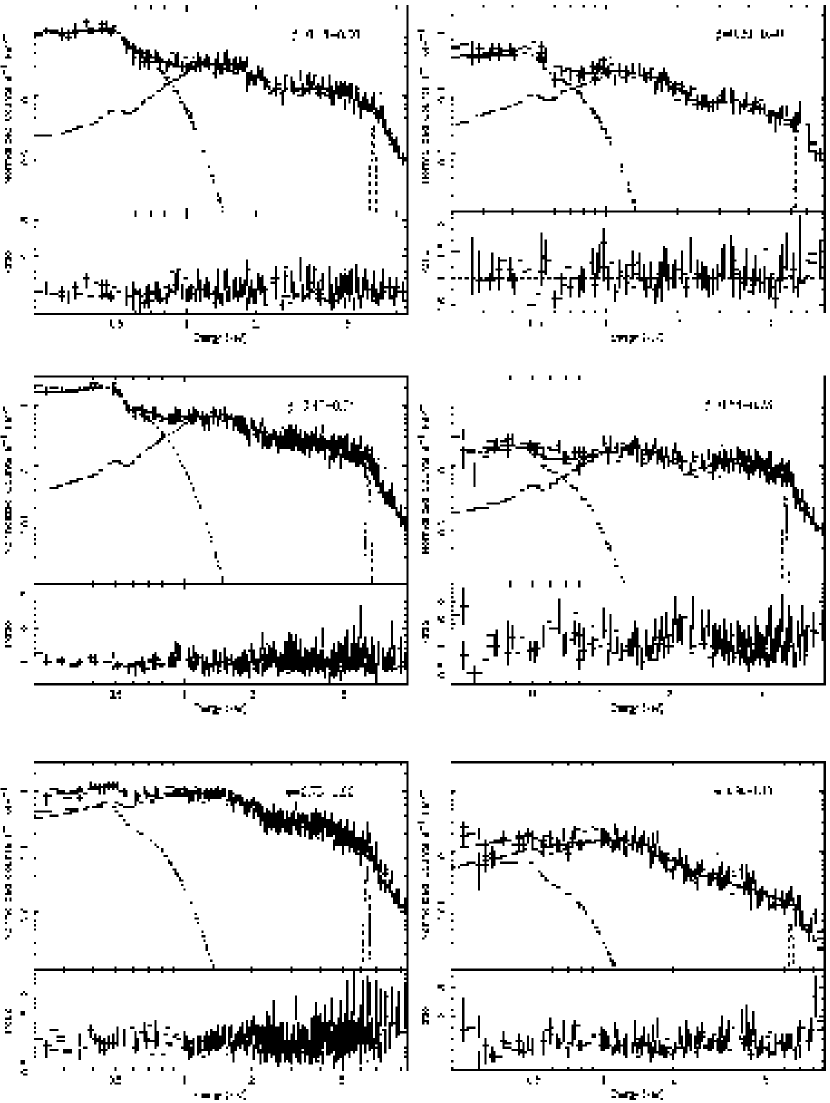
5 Spin Phase Resolved X-ray Spectroscopy

To gain a better insight into the spectral behavior of the source as a function of the spin phase, we analyze the spectra extracted for six unequal phase intervals, i.e., $\phi$=0.18–0.30, $\phi$=0.30-0.40, $\phi$=0.40–0.54, $\phi$=0.54–0.73, $\phi$=0.73–0.90 and $\phi$=0.90–1.18. This division ensures that spectra in each phase interval have sufficient counts to provide reliable values of different spectral parameters. Since the use of model B requires a higher resolution data to provide an accurate information about the line parameters, and model A (see §4.1) along with other model components as employed to describe the average spectra provides a good description of an accretion column in a polar, we have used model A to fit the phase-resolved spectra. During the fit to phase resolved spectra the black body temperature is kept fixed at 88 eV obtained from the phase averaged spectral fit. Allowing the black body temperature to vary adjusts the value of other parameters like absorbing column densities and the covering fraction and gives only a slightly better fit with $\Delta\chi^{2}$=9, 13, 16, 17, 55, 22, and 20, respectively for each of the phase intervals listed in Table 2. However, variation of the black body temperature with the spin phase is not very likely. The jointly fitted MOS spectra corresponding to all six phase intervals, along with the individual best fit model components are plotted in Figure 12. The values of the best fit spectral parameters obtained from the phase resolved spectral analysis are also listed in Table 2. The degrees of freedom are different for each spectrum, because the binning procedure requires a minimum of 20 counts per bin. Several spectral parameters show variations over the spin cycle (see Table 2), and are shown plotted in Figure 13 as a function of the spin phase. Variations in the average intensity, the absorption components: $N_{H1}$, the column density due to an absorber fully covering the source; $N_{H2}$, the column density due to an absorber partially covering the source; the covering fraction $C_{f}$ associated with $N_{H2}$, and the 6.4 keV line flux are shown. The $N_{H1}$ value remains almost constant at $\sim$$2.4\times 10^{21}$ cm^-2 during phase 0.18–0.73 except for $\phi$=0.3–0.4 during which it is at a lower value of $0.9\times 10^{21}$ cm^-2. The $N_{H2}$ value remains low and roughly constant at an average value of $\sim$ $1.1\times 10^{23}$ cm^-2 during most of the spin cycle (i.e. $\phi$=0.18–0.90) but shows a very high value of $7.6^{+3.0}_{-4.1}$ $\times 10^{23}$ cm^-2 during the last spin phase interval of 0.90–1.18. The $C_{f}$ value is the same within the error bars during the phase range 0.9–1.54 but is anti-correlated with the intensity during the rest of the spin cycle. The variation in the line flux is correlated with the average change in the source intensity.

6 Discussion

6.1 Power Spectra and the Spin Period

Several prominent peaks at frequencies corresponding to various periods related to the system have been identified. A peak at a period of 12150.72$\pm$1.14 s has been observed in the $ROSAT$ power spectra (Fig. 1). This value agrees well with the determinations of the spin period ($\omega$) based on X-ray and optical photometry of V1432 Aql as reported by Friedrich et al. (1996) (12150.7$\pm$0.5 s based on the $\chi^{2}$ period search method), Staubert et al. (2003) (12150.328$\pm$0.045 s), and Mukai et al. (2003a) (12150.432 s). With this presumed spin period, the dominant peak in the $XMM$-$Newton$ power density spectra can be interpreted as due to the second harmonic of the spin period. The circular polarization data show a dominant peak at the one day alias of the first harmonic of $\omega$ in the power density spectrum. Smaller peaks at the fundamental frequency and higher harmonics are also visible in the polarization data. Thus the optical polarization is consistent with the presence of the fundamental period of 12150 s.

The power spectra for the $ROSAT$ medium energy bands also show a peak at the spin frequency $\omega$, but with a relatively smaller amplitude as compared to the total energy band power spectrum. The X-ray power spectra are strongly dependent on some of the geometrical parameters of the system, e.g. the inclination angle ($i$) and the magnetic co-latitude ($\beta$). In addition, for asynchronous polars, there will also be an effect from its non-synchronous rotation, since the accretion stream interacts with different field lines as the white dwarf rotates. Moreover, if the time interval over which the power spectrum is calculated, is reasonably longer than the beat period of the system, then the power spectrum is expected to be dominated by side band frequencies of the fundamental periods instead of the fundamental periods themselves. According to Wynn & King (1992) the power spectra of asynchronous polars with high values of $i$ and $\beta$, show strong peaks at 2$\omega$-$\Omega$ and $\Omega$ components. The 2$\omega$-$\Omega$ component is prominent in the power spectrum from the medium energy $ROSAT$ data, whereas it has relatively smaller power in the power spectrum of the total energy band. This component is merged with the $\omega$ and $\Omega$ frequency components in the power spectrum from $XMM$-$Newton$ data (Fig. 2). This side band component was also observed in the power spectra of the two other asynchronous polars BY Cam (Mason et al. 1998) and RX J2115-5840 (Ramsay et al. 1999) in the optical data. The presence of this component suggests a diskless accretion geometry for asynchronously rotating MCVs (Wynn & King 1992).

Although there are three clear humps during the 12150 s period in the $XMM$-$Newton$ and $ASCA$ light curves, the repetitive appearance of these features is preserved with roughly the same time structure (see Fig.1 of Paper 1). This recurrence of the features in the light curve dominates over the 12150 s periodicity as the true spin period, leading to a dominant peak in the power spectrum at the frequency corresponding to the second harmonic of the spin period (i.e. 3$\omega$ component at $\sim$4050 s; see Fig. 2) rather than at the true spin period of 12150 s. This kind of intensity variation and the appearance of the dominant power at $\sim$4050 s period led Mukai (1998) (and Singh & Rana 2003) to suggest that V1432 Aql may be an IP with a $\sim$4050 s spin period. However, the present analyses of X-ray timing data, spectra, and optical polarization data are consistent with V1432 Aql being an asynchronous polar and not an IP.

6.2 Possible Accretion Geometries For V1432 Aql

V1432 Aql shows varying light curve profiles with a double hump structure during the $ROSAT$ observations in 1992–1993 changing to a triple hump structure during the $ASCA$ and $XMM$-$Newton$ observations in 1997 and 2001. The circular polarization data taken in 1994 shows a double humped profile bearing a striking resemblance to the soft X-ray $ROSAT$ light curves. The occurrence of both the negative and the positive value of the circular polarization strongly suggests the presence of two sites of polarization that are viewed alternately, indicating the presence of two magnetic poles in V1432 Aql.

Staubert et al. (2003) showed that the accretion process in V1432 Aql can be described using a dipole accretion model (also see Geckeler & Staubert 1997), and fitted their model to the optical and the X-ray data from $ROSAT$ that show a double hump profile. The appearance of the two broad humps in the $ROSAT$ soft X-ray light curves results when the X-ray emitting regions are in direct view crossing the line-of-sight alternately. In between the appearance of the humps the emitting regions are out of view or viewed through absorbing material that is almost opaque to X-rays below 0.5 keV. On the other hand, the 0.5–2 keV X-ray light curves during the rest of the spin cycle show a comparatively higher and variable intensity, indicating that X-rays above 0.5 keV manage to escape from the absorbing material. The observed separation of the $\sim$0.65 spin phase between the two humps (in the first three panels of Fig. 4) suggests that the two accretion foot prints are separated by $\sim$234^∘. Thus, the accretion via two poles with the two hot spots that are not anti-podal can explain the intensity variation in the $ROSAT$ light curves. During the $ROSAT$ 1993 October observations each of the two humps representing the two accretion spots appear to split into two owing to the presence of two dips (at $\phi$=0.12 and 0.8).

The triple hump profiles of the $ASCA$ and $XMM$-$Newton$ data are difficult to explain using the two pole accretion model with two off-centered hot spots. To accommodate them in a two pole accretor model, the two nearby humps around spin phases 0.2 and 0.45 in $XMM$-$Newton$ light curves, could represent one dominant pole that is split into two because of the presence of a narrow dip and the other hump at $\phi$=0.8 represent the second pole. This dip could be due to absorption by the accretion stream or a split or double stream system. If the two close peaks represent one dominant pole, then this implies that the pole remains in view for almost half the spin cycle, whereas the $ROSAT$ data show that the same pole is only visible for 0.2 of the spin phase. It is not clear why the dominant pole remains in view for a longer time during the $ASCA$ and the $XMM$-$Newton$ observations. The dip at the $\sim$0.35 spin phase is equally prominent in all the energy bands showing little X-ray emission. Therefore, the possibility of a split or double stream system is more likely the cause for the appearance of the triple hump in the $ASCA$ and $XMM$-$Newton$ data, and not the absorption. The phase resolved spectroscopy presented in §5 (Fig. 13) also favors this interpretation as no extra absorption is seen during this phase range. The second spot is visible during $\phi$=0.7–0.9 when the first goes behind the surface of the white dwarf. The location and the extent of the second hot spot in the $ASCA$ and the $XMM$-$Newton$ are very similar to that in the $ROSAT$ data. The low intensity during $\phi$=0.6–0.7 and 0.90–1.18 is associated with a high absorption and a large covering fraction by a very thick absorber. The highest intensity peak centered at phase 0.8 has the smallest covering fraction of the source by an absorber, and gives the least hindered view toward the accreting pole.

The spin folded circular polarization data support a complex magnetic field geometry with three hot spots. The two positive humps observed in the circular polarization data (near phase 0.1 and 0.7) indicate the same magnetic polarity for the two emission regions and a negative polarization near phase 0.45 suggests another hot spot with opposite polarity. In this scenario, the two humps at phase 0.25 and 0.85 in the $XMM$-$Newton$ light curve represent two hot spots with the same polarity and the third at phase 0.50 represents a region with opposite polarity. The different amplitudes of the two positive humps in the polarization suggest different magnetic field strengths for the two poles with the same polarity. The peak at phase 0.7 has relatively higher polarization, suggesting a higher magnetic field strength and hence lower accretion on that pole (see Stockman 1988 and Wickramasinghe & Ferrario 2000), resulting in lower X-ray emission near phase 0.85 (a small phase shift is likely due to two different ephemerides used). The other pole with a relatively smaller magnetic field corresponds to higher X-ray intensity (near phase 0.25). The hot spot with opposite polarity shows a smaller circular polarization and hence corresponds to the higher X-ray intensity (near phase 0.50). The separation between the three humps in $XMM$ data suggests that the first two spots are about 90^∘ apart and the second and the third spots are further $\sim$126^∘ apart in longitude. Thus, the recent X-ray and circular polarization data suggest a field geometry with at least three hot spots on the surface of the white dwarf.

A similar variation in the circular polarization data is also observed in the polar EF Eri (Piirola, Reiz, & Coyne 1987). Meggitt & Wickramasinghe (1989) proposed a dominant quadrupole field structure with four active spots on the surface of the white dwarf for EF Eri using optical polarimetric data. Mason et al. (1995) provided evidence for the presence of multi-pole magnetic field structure in another asynchronous polar BY Cam. Thus, the presence of more than two accretion spots on the surface of the white dwarf is not an uncommon characteristic of polars.

The difference in the morphology of X-ray light curves from the $ROSAT$ and $XMM$-$Newton$ (or $ASCA$) data can well be due to the beat period. If we choose the zero of the beat phase at the starting time of the $ROSAT$ 1992 observation and a beat period of 49.8955 days, then the beat phases for the start time of the $ROSAT$ 1993 March and October, optical polarization data, $ASCA$ 1997 October, $XMM$-$Newton$ 2001 October, and $RXTE$ 2002 July 14 and 15 are 0.48, 0.42, 0.73, 0.98, 0.88, 0.46 and 0.48, respectively. If the different X-ray profiles are due to the different beat phases of the observations then the transition from the double hump to the triple hump profile most likely occurs between beat phases 0.5–0.7. This conclusion is not affected even if we consider the spin up of the white dwarf in estimating the beat phases.

6.3 X-ray Spectrum

The low and medium resolution X-ray spectra of V1432 Aql obtained with the $RXTE$ and the $XMM$-$Newton$ can be reproduced using either a multi-temperature plasma model with multiple absorbers or a photo-ionization model. The phase-averaged spectra from the $RXTE$ extend to $\sim$30 keV and can be modeled by a simple bremsstrahlung with kT$\geqslant$90 keV (90% confidence limit). This temperature is among the highest seen in MCVs. The use of a multi-temperature plasma model for the $RXTE$ data gives an estimated mass of the white dwarf of 1.2$\pm$0.1 M_⊙. This is similar to that of PQ Gem, a soft IP, for which James et al. (2002) report a mass of $1.21^{+0.07}_{-0.05}$ M_⊙ using the $RXTE$ data and the same multi-temperature plasma model. The high mass estimate of the white dwarf is consistent with the idea that V1432 Aql might have undergone a nova explosion in not too distant past. This is also consistent with the observed asynchronism in the system. The medium resolution $XMM$-$Newton$ spectra can be reproduced using this mass estimate in the multi-temperature plasma model. The multi-temperature plasma produced in the post-shock region must, however, be viewed through two absorbers – a thin absorber of (1.7$\pm$0.3) $\times 10^{21}$ cm^-2 covering the entire source and a thick absorber of ($1.3^{+0.2}_{-0.1}$) $\times 10^{23}$ cm^-2 covering 65% of the hard X-ray emission. Since the plasma emission originates in the post-shock region, these absorbers are most probably situated in front of the post-shock region or in the pre-shock flow. The abundance of Fe in the plasma is found to be nearly solar (except during the lowest intensity phase) and provides a good fit to the emission lines at 6.7 and 7.0 keV (see inset in Fig. 9).

Alternatively, a photo-ionization model can also reproduce the MOS spectra. Photo-ionization models have recently been successful in explaining the high resolution $Chandra$ HETG spectra of IPs, and in fact might be preferred over the multi-temperature plasma models like those used for cooling flows (Mukai et al. 2003b). Although the photo-ionization model has a slight edge (in terms of $\chi^{2}_{min}$) over the multi-temperature plasma models used here, higher resolution grating spectra of V1432 Aql are required to decide between the two models. The important differences between the two models are seen in excitation lines (e.g., N VI, O VII-VIII, Ne IX-X, Mg XI-XII, Si XIII-XIV, and Fe L-shell emission lines). Therefore higher resolution data are important to resolve the line emission from these elements that occur at low energies (below $\sim$2 keV; Mukai et al. 2003b). However, the photo-ionization model can successfully reproduce the three Fe line components at 6.4, 6.7, and 7.0 keV without requiring a separate Gaussian component for modeling the line at 6.4 keV, as with the multi-temperature plasma model, but it requires extremely large ionic column densities for the Fe ions (see Table 3). The 6.7 keV and 7.0 keV lines provided a reasonably good fix for the column densities of Fe XXV and Fe XXVI ions. The strong line emission observed at 6.4 keV can only be reproduced by having a large column for Fe I–XIX ions. Lack of resolution in the present spectra, does not allow us to derive the individual column densities of all the ions in the photo-ionized regions. The ionic column densities derived for Fe I–XIX ions are tentative and likely to be overestimates. In addition, the use of the input power law continuum is not well known and the ionic column densities for Fe are adjusted to fit the observed lines.

The thermal plasma models (a simple bremsstrahlung or multi-temperature plasma) require an additional Gaussian component at 6.4 keV, which is presumably due to fluorescent emission from (cold or warm) Fe. The fit with the multi-temperature plasma model shows that the Fe line at 6.4 keV has some intrinsic line width indicating the presence of warm (partially ionized) Fe in addition to cold (or un-ionized) Fe. Alternatively, the width of 6.4 keV line can also be due to the velocity broadening but present data can not distinguish between these two mechanisms. The photo-ionized plasma model supports this trend and explicitly demonstrates the need for high column densities for Fe I–XIX. The variations in Fe 6.4 keV line flux closely resemble the variations in the average X-ray intensity in 0.2–10 keV energy band, further indicating that the spin period is 12150 s.

6.4 White Dwarf Mass Determination Using Fe K_α Lines

The mass of the white dwarf can also be estimated using the intensity ratio of K_α emission lines from abundant heavy elements, as described by Fujimoto & Ishida (1997). For a plasma in collisional ionization equilibrium (CIE), the intensity ratio of H to He-like K_α lines is a function of the plasma temperature (Mewe et al. 1985). The plasma temperature is directly related to the gravitational potential of the white dwarf. Therefore, the mass of the white dwarf can be estimated using the mass-radius relationship (Nauenberg 1972), if the plasma temperature is known. Here we use only the Fe K_α lines as lines from other element are not resolved. This method is independent of the uncertainties in geometrical parameters like inclination angle and the mass-radius relationship of the secondary star. The intensity ratio of H to He-like Fe K_α line is $\sim$0.83 for V1432 Aql (see §4.1). A similar value ($\sim$0.9) for the line intensity ratio of Fe K_α lines is reported by Fujimoto (1996) for the IP, V1223 Sgr. This corresponds to a lower limit of $\sim$38 keV for the shock temperature and a lower limit of 0.82M_⊙ for the white dwarf mass in V1223 Sgr. V1432 Aql shows a very hard X-ray spectrum and similar line intensity ratio for the H to He-like Fe K_α lines suggesting a similar lower limit for the mass of the white dwarf that is consistent with the higher mass derived from the $RXTE$ spectrum. It should be noted that this method is based on the assumption that the cooling in the post-shock region is entirely due to the bremsstrahlung process and the contribution from cyclotron cooling is not significant, hence it is more suitable for IPs. In the case of polars, it can only provide a lower limit to the mass of the white dwarf. On the other hand, the mass determined using the multi-temperature plasma model is perhaps more reliable, since it takes in to account the cyclotron cooling effects (see §4.1). From the observed duration of the eclipse in V1432 Aql, Mukai et al. (2003a) estimated an upper limit of 0.67M_⊙ for white dwarf mass. Our mass estimate obtained using the X-ray continuum and the line spectroscopy methods differ significantly from Mukai’s estimate, and is close to that of 0.98M_⊙ reported by Ramsay (2000) using spectral fitting of the X-ray continuum.

6.5 Blackbody Temperature

A strong blackbody component dominates the soft X-ray energies below 0.8 keV irrespective of the models used for the higher energy spectra. This component has an average temperature between 80–90 eV, which is significantly higher than what is generally observed in polars (20–40 eV) (Ramsay et al. 2004a and references therein). A somewhat higher blackbody temperature in the range of 50–60 eV has been reported in a few soft IPs, namely, V405 Aur and PQ Gem by Haberl & Motch (1995) using $ROSAT$ data. Recently, de Martino et al. (2004) have reported the blackbody temperatures in the range of 60–100 eV for three soft IPs (V405 Aur, PQ Gem and V2400 Oph) using broad band (0.1–90 keV) observations with $BeppoSAX$. A blackbody temperature of 86 eV is reported for another soft IP 1RXS J154814.5-452845 by Haberl, Motch & Zickgraf (2002). Thus, V1432 Aql shows a blackbody temperature similar to that observed in soft IPs. High blackbody temperature indicates that the accretion is taking place over a much smaller fractional area on the surface of the white dwarf. But this is a too simplistic picture, since accretion regions in polars are generally smaller than that in IPs. The blackbody temperature is also high for soft IPs, but they cannot necessarily have smaller accretion regions than polars.

6.6 Energy Balance

The standard model for MCVs predicts a ratio of intrinsic soft X-ray luminosity to the hard component to be $\sim$0.5, including the cyclotron emission component (Lamb & Masters 1979 and King & Lasota 1979). Several polars show this ratio to be higher than that predicted by the standard model, leading to the well-known ‘soft X-ray excess’ problem. On the other hand, IPs typically show a ratio in agreement with the standard model or somewhat lower than that predicted. A study of this ratio can provide valuable information about the energy balance in these systems. We have listed in Table 4 the unabsorbed soft and hard X-ray fluxes and the corresponding luminosities (assuming d=230 pc; Watson et al. 1995) in the 0.2–1 keV and 1–10 keV energy bands, respectively. We have also calculated the unabsorbed bolometric flux and luminosity for the blackbody component and listed them in Table 4. Since the blackbody component is assumed to be optically thick emission, one has to apply a geometric correction factor $sec(\theta)$ to account for projection effects, where $\theta$ is the angle between normal to the accretion region and the line of sight. For an inclination angle ($i$) of 75^∘ and magnetic co-latitude ($\beta$) of 15^∘ (Mukai et al. 2003a), the value of $\theta$ (=$i$-$\beta$) is 60^∘, which corresponds to a correction factor of 2. We apply this correction factor for estimating the average unabsorbed bolometric luminosity due to the blackbody (2.0 $\times$ 10³¹ ergs s^-1). The unabsorbed hard X-ray flux in the 1–10 keV energy band is 2.13 $\times$ 10^-11 ergs cm^-2 s^-1 and corresponds to luminosity of 1.27 $\times$ 10³² ergs s^-1. This gives a ratio of the soft to hard X-ray luminosity of $\sim$0.16, a comparatively lower value than predicted by the standard model. The photo-ionized plasma model gives a comparatively higher value for the hard X-ray luminosity and a similar value for the soft X-ray bolometric luminosity as obtained from multi-temperature plasma model, thus, further reducing the ratio for soft to hard X-ray luminosity to 0.14. These values of ratio for soft to hard X-ray luminosity should be taken as upper limits since the contribution from cyclotron emission is not included because the cyclotron spectra were not available. Ramsay et al. (1994) showed that this ratio is correlated with magnetic field strength, and a low observed value for the ratio indicates a low value for magnetic field strength. A recent study by Ramsay & Cropper (2004b) using $XMM$-$Newton$ data for a sample of polars shows no evidence of such a correlation and instead shows that $\sim$53% of all the polars studied in the sample show the ratio to be $<$1.

6.7 The Shock Height

Theoretical models predict that the shock height in an accretion column can be described in terms of the mass accretion rate and the fractional accreting area by the relationship

$$H=5.45\times 10^{8}\dot{M}_{16}^{-1}f_{-2}M_{WD}^{3/2}R_{WD}^{1/2}$$ (1)

(Frank, King & Raine 1992), where $\dot{M}_{16}$ is the mass accretion rate in units of 10¹⁶ g s^-1, $f_{-2}$ is the fractional area in units of 10^-2, M_WD and R_WD are the mass and the radius of white dwarf in solar units respectively.

The accretion rate $\dot{M}$ can be estimated assuming that the accretion luminosity is emitted mostly in the X-rays and is given by,

$$L_{acc}=\frac{GM_{WD}\dot{M}}{R_{WD}}$$ (2)

This requires an estimation for the accretion luminosity L_acc and R_WD. The unabsorbed X-ray luminosity obtained from the $RXTE$ spectral fit in the extended high energy band of 2–60 keV is $1.1\times 10^{33}$ ergs s^-1. The spectral fit to the $XMM$-$Newton$ data using the same model gives an average soft X-ray bolometric luminosity of $5.6\times 10^{31}$ ergs s^-1 after scaling the normalization with respect to the $RXTE$ spectral fit. The total accretion luminosity for the soft and hard X-ray energy bands is $1.1\times 10^{33}$ ergs s^-1. The radius of the white dwarf, R_WD, can be estimated using the mass-radius relationship as given by Nauenberg (1972) and the estimated mass of the white dwarf (1.2M_⊙; see §4.1). This gives a corresponding radius of the white dwarf of 3.8 $\times 10^{8}$ cm ($\sim$0.005R_⊙). Substituting these values in equation (2) and solving it for $\dot{M}$ gives a mass accretion rate of $2.7\times 10^{15}$ g s^-1.

The above estimated values of the parameters R_WD, $\dot{m}$, and $\dot{M}$ enable us to calculate the value of the fractional area f as $1.5\times 10^{-3}$. Finally, substituting the values of $\dot{M}$, $f$, M_WD and R_WD in equation (1), gives a value for the shock height as H=$2.9\times 10^{7}$ cm (0.08R_WD). However, propagating the errors on the accretion luminosity, the total accretion rate, the mass and radius of the white dwarf provide an upper limit on shock height to be $\sim$$5\times 10^{7}$ cm. James et al. (2002) estimate an upper bound on shock height to be $5.4\times 10^{7}$ cm for the PQ Gem. The higher shock height in PQ Gem is due to the larger fractional accreting area ($f$=$9\times 10^{-3}$), since the mass and radius of the white dwarf are about the same for both sources. A smaller accreting area for V1423 Aql is consistent with a comparatively higher blackbody temperature (88 eV) than that of PQ Gem (56 eV; de Martino et al. 2004).

7 Conclusions

From our timing study of X-ray and optical emission, and spectral study of X-ray emission of V1432 Aql, we draw the following conclusions:

1. The power spectrum in the 0.1–2 keV energy band obtained from the combined 1 year long $ROSAT$ observations shows a peak at the period ($\omega$) of 12150.72$\pm$1.14 s that is close to the value known from optical photometry and identical to the spin period of the system. A significant power is also detected in the $\Omega$+$\omega$ component.

2. The power spectrum obtained from the $XMM$-$Newton$ observation shows a dominant peak at $\sim$4050 s that is likely due to the complex X-ray light curve with a triple hump profile. The strict recurrence of X-ray features at the period of 12150 s suggest that 12150 s is the likely spin period instead of 4050 s.

3. The power spectrum from the optical circular polarization data shows prominent peaks corresponding to the first harmonic of the spin period as well as its one day alias. The fundamental period and several other harmonics are also seen. Two maxima are seen in circular polarization data in each spin cycle, which explains why the first harmonic of the spin period is more prevalent than the fundamental.

4. The spectral analysis and observed intensity of the H-like to the He-like Fe K_α lines indicate a high mass for the white dwarf.

5. Variations seen in the X-ray intensity in the $ROSAT$ data can be explained using a two pole accretion model in which two accretion foot prints are not anti-podal. However, the triple hump profile seen in the $XMM$-$Newton$ and the $ASCA$ light curves requires three hot spots on the surface of the white dwarf. Supportive evidence for the three spots comes from the X-ray phase resolved spectroscopy and the polarization data.

6. The X-ray spectral study suggests the presence of a strong black body component with an average temperature of $\sim$88 eV. This is significantly higher than commonly observed in polars and is close to that observed in soft IPs.

7. The originating site for the 6.4 keV Fe fluorescent line in V1432 Aql most likely contains both neutral (cold) and partially ionized (warm) Fe ions. Velocity broadening can also be responsible for 6.4 keV line width but present data can not distinguish between the two possibilities.

8. Both the multi-temperature plasma and the photo-ionization plasma models fit the spectral data with the photo-ionization model providing a slightly better fit. The photo-ionization model, however, has several parameters that need a higher spectral resolution for their determination.

Figure 1: Power density spectra of V1432 Aql in the energy range 0.1–2 keV from combined $ROSAT$ observations. First three panels show power spectra obtained using discrete Fourier transform, Lomb-Scargle Periodogram, and Bayesian method, respectively. The bottom panel shows a CLEANed power density spectrum. Various identified frequency components are marked.

Figure 2: Power density spectrum of V1432 Aql obtained from a long continuous $XMM$-$Newton$ observation in the 0.2–2 keV energy band. Various identified components are marked.

Figure 3: Power density spectrum obtained using discrete Fourier transform of optical circular polarization data taken from $SAAO$ during 1994 July 5–13. The expected positions of frequency components corresponding to spin period, and its various harmonics are marked along with a one day positive alias of 2$\omega$ component.

Figure 4: Spin folded X-ray light curve from the $ROSAT$ (first three panels; 0.1–0.5 keV energy band) and the $XMM$-$Newton$ (bottom panel; 0.2–0.5 keV energy band) observations (see Table 1). For folding the data, we have used the ephemerides for the spin period as given by Staubert et al. (2003) (dash-dotted line) and Mukai et al. (2003a) (solid line curve in bottom panel). The bin time is $\sim$100 s throughout. Two phase cycles are shown for clarity.

Figure 5: Spin folded X-ray light curves from the $ROSAT$ (first three panels; 0.5–2 keV energy band), the $ASCA$ (panel four; 0.7–2 keV energy band) and the $XMM$-$Newton$ (bottom panel; 0.5–2 keV energy band) observations. Same ephemerides with the same line styles, as used in Fig. 4, are used here for folding the data. The bin time is $\sim$100 s throughout.

Figure 6: Hard X-ray spin folded light curves in the 2–10 keV energy band from the $ASCA$, the $XMM$-$Newton$ and the $RXTE$ observations. For folding the data, the spin ephemeris as given by Mukai et al. (2003a) has been used. The bin time is $\sim$100 s.

Figure 7: Spin folded polarization data in the optical band obtained from the $SAAO$ during 1994 July 5–13. The data have been folded using the spin ephemeris as given by Staubert et al. (2003). The bin time is $\sim$243 s.

Figure 8: $RXTE$ PCA spectra and the best fit multi-temperature plasma model with a Gaussian line component (top), and the ratio of the data to the best fit model (bottom).

Figure 9: The EPIC MOS1 and MOS2 spectra and the best fit model. The top panel shows data fitted with a best fit model consisting of a blackbody, an absorbed multi-temperature plasma (Cropper et al. 1999), and a Gaussian emission line. The additive components are shown individually. The bottom panel shows the ratio of the data to the best fit model and the inset shows a magnified view of the energy range containing the Fe K_α line complex.

Figure 10: Same as in Fig. 9, but for the photo-ionized plasma model.

Figure 11: Ratio of the data to the multi-temperature plasma+Gaussian line model without a blackbody component for the average MOS spectra in the energy range 0.2–10 keV (top) and for the photo-ionized plasma model without blackbody component (bottom). A clear excess in soft X-rays (below 0.8 keV) is visible in both cases.

Figure 12: Phase resolved MOS spectra of V1432 Aql corresponding to the six unequal intervals of the spin cycle, along with the individual components of the best fit model (top panels). The ratio of the data to the best fit model for each spectra is plotted in the bottom panels. The corresponding phase ranges are labeled for each spectra.

Figure 13: Variation of spectral parameters (see text) as a function of spin phase. The intensity variation is shown in the top panel. The second panel from top shows change in the column density $N_{H1}$ due to an absorber fully covering the source. Variations in the column density, $N_{H2}$, due to a partial covering of the source and the associated covering fraction are plotted in the third and fourth panels from the top, respectively. The bottom panel represents a change in the flux of the Fe 6.4 keV line. Errors plotted are with 90% confidence.

Table 1: Summary of the X-ray Observations of V1432 Aquilae.

Start Time	End Time	Satellite	Exposure	Mean Count rate
(UT)	(UT)		ks	(Count s-1)
(1)	(2)	(3)	(4)	(5)
1992 Oct 08, 2001	Oct 30, 1732	$ROSAT$	29.6	0.065
1993 Mar 31, 0723	Apr 02, 0935	$ROSAT$	38.2	0.040
1993 Oct 13, 2252	Oct 18, 1007	$ROSAT$	23.5	0.055
1997 Oct 27, 2025	Oct 29, 0010	$ASCA$	34.2	0.04
2001 Oct 09, 0051	Oct 09, 0755	$XMM$	25.2	0.7
2002 Jul 14, 0853	Jul 14, 1313	$RXTE$	9.4	13.0
2002 Jul 15, 1016	Jul 15, 1432	$RXTE$	10.2	10.0

Table 2: Best fit values of spectral parameters.

Spin	$N_{H1}$	$N_{H2}$	Covering	Abundance	Normalization	AFe	$\chi^{2}_{min}$($\nu$)
Phase	($\times 10^{21}$ cm-2)	($\times 10^{23}$ cm-2)	fraction		($\times 10^{-7}$)
Average	$1.7^{+0.3}_{-0.3}$	$1.3^{+0.2}_{-0.1}$	$0.65^{+0.01}_{-0.01}$	$0.7^{+0.2}_{-0.2}$	11.2	$4.3^{+0.8}_{-0.8}$	1.35(736)
0.18–0.30	$2.6^{+0.5}_{-0.4}$	$1.4^{+0.3}_{-0.3}$	$0.64^{+0.02}_{-0.03}$	$0.8^{+0.2}_{-0.4}$	10.2	$4.5^{+1.8}_{-2.3}$	1.06(275)
0.30–0.40	$0.9^{+0.6}_{-0.7}$	$1.2^{+0.5}_{-0.5}$	$0.59^{+0.04}_{-0.07}$	$1.6^{+1.1}_{-0.8}$	4.59	$3.1^{+2.2}_{-2.1}$	1.13(166)
0.40–0.54	$2.6^{+0.3}_{-0.3}$	$1.4^{+0.3}_{-0.2}$	$0.62^{+0.01}_{-0.03}$	$0.9^{+0.2}_{-0.3}$	18.9	$8.7^{+2.5}_{-2.2}$	1.19(507)
0.54–0.73	$2.0^{+0.5}_{-0.6}$	$1.3^{+0.2}_{-0.2}$	$0.83^{+0.01}_{-0.01}$	$0.6^{+0.3}_{-0.3}$	12.3	$4.6^{+1.7}_{-1.9}$	1.19(318)
0.73–0.90	$0.0^{+0.1}$	$0.4^{+0.1}_{-0.1}$	$0.52^{+0.02}_{-0.02}$	$0.7^{+0.3}_{-0.3}$	15.6	$6.9^{+1.9}_{-1.9}$	1.34(543)
0.90–1.18	$0.0^{+0.1}$	$7.6^{+3.9}_{-5.3}$	$0.79^{+0.11}_{-0.17}$	$0.1^{+0.5}_{-0.1}$	6.3	$1.9^{+1.9}_{-1.5}$	1.30(234)
	$0.0^{+0.1}$	$2.8^{+4.2}_{-1.6}$	$0.49^{+0.26}_{-0.13}$	0.7 (fixed)	2.3	$1.5^{+1.2}_{-0.8}$	1.31(235)

Note. — Data for MOS1 and MOS2 were fitted simultaneously using the multi-temperature plasma model as described by Cropper et. al. (1999). The error bars are with 90% confidence limit for one parameter. All values are for the multi-temperature plasma model (Cropper et al. 1999) and a black body component with kT_bb=$88\pm 2$ eV for the average spectrum and frozen at 88 eV for the phase resolved spectra.

Table 3: Best fit spectral parameters.

Phase	kTbb	Column densities for Fe ions (cm-2)					$\Gamma$	$\chi^{2}_{min}$($\nu$)
	(eV)	Fe I–XVI	Fe XVII–XIX	Fe XX–XIV	Fe XXV	Fe XXVI
Average	$80^{+1}_{-2}$	$8\times 10^{18}$	$3\times 10^{18}$	$3\times 10^{17}$	$2\times 10^{18}$	$3\times 10^{18}$	$0.64^{+0.01}_{-0.02}$	1.28(740)

Note. — All values are for the photo-ionized plasma model as described by Kinkhabwala et al. (2003)

Table 4: Soft and hard X-ray flux and luminosity of V1432 Aql.

Phase	Flux			Luminosity			Luminosity
	Soft	Soft	Hard	Soft	Soft	Hard	Ratio
	(0.2–1 keV)	Bolometric	(1–10 keV)	(0.2–1 keV)	Bolometric	(1–10 keV)	Soft/Hard
Average	0.54	0.66	2.13	0.16	0.20	1.27	0.13(0.16)
0.18–0.30	0.34	1.09	1.92	0.10	0.33	1.15	0.09(0.28)
0.30–0.40	0.17	0.50	1.06	0.05	0.15	0.63	0.08(0.24)
0.40–0.54	0.56	1.74	3.67	0.17	0.52	2.20	0.08(0.24)
0.54–0.73	0.07	0.13	1.99	0.02	0.04	1.19	0.02(0.03)
0.73–0.90	0.39	0.73	4.05	0.12	0.22	2.42	0.05(0.09)
0.90–1.18	0.06	0.11	0.52	0.02	0.03	0.31	0.06(0.10)

Note. — The values listed here are based on the multi-temperature plasma model. The soft X-ray luminosity is defined as $L_{soft}$=$\pi$ $F_{soft}$ sec($\theta$) d² (Ramsay & Cropper 2004b), where $F_{soft}$ is unabsorbed flux of the soft X-ray component and $d$ is the distance of the source. The hard X-ray luminosity is defined as $L_{hard}$=4$\pi$ $F_{hard}$ d², where $F_{hard}$ is unabsorbed flux of the hard X-ray component (d=230 pc).

References

- Aizu (1973) Aizu, K., 1973, Prog. in Theor. Phys., 49, 1184
- Anders (1989) Anders, E., & Grevesse, N., 1989, Geochimica et Cosmochimica Acta, 53, 197
- Balucinska-Church (1992) Balucinska-Church, M., & McCammon, D., 1992, ApJ, 400, 699
- Cropper (1985) Cropper, M., 1985, MNRAS, 212, 709
- Cropper (1998) Cropper, M., Ramsay, G., & Wu, K., 1998, MNRAS, 293, 222
- Cropper (1999) Cropper, M., Wu, K., Ramsay, G., & Kocabiyik, A., 1999, MNRAS, 306, 684
- de Martino (2004) de Martino, D., Matt, G., Belloni, T., Haberl, F., & Mukai, K., 2004, A&A, 415, 1009
- den Herder (2001) den Herder, J. W. et al., 2001, A&A, 365, L7
- Done (1995) Done, C., Osborne, J. P., & Beardmore, A. P., 1995, MNRAS, 276, 483
- Frank (1992) Frank, J., King, A. R., & Raine, D. J., 1992, Accretion Power in Astrophysics, (Cambridge:Cambridge Univ. Press)
- Friedrich (1996) Friedrich, S., et al., 1996, A&A, 306, 860
- Fruscione (1994) Fruscione, A., Hawkins, I., Jelinsky, P., & Wiercigroch, A., 1994, ApJS, 94, 127
- (13) Fujimoto, R., 1996, Ph.D. Thesis, University of Tokyo
- (14) Fujimoto, R., & Ishida, M., 1997, ApJ, 474, 774
- Geckeler (1997) Geckeler, R. D., & Staubert, R., 1997, A&A, 325, 1070
- Haberl (1995) Haberl, F., & Motch, C., 1995, A&A, 297, L37
- Haberl (2002) Haberl, F., Motch, C., & Zickgraf, F., J., 2002, A&A, 387, 201
- Horne (1986) Horne, J. H., & Baliunas, S. L., 1986, ApJ, 302, 757
- Jahoda (1996) Jahoda, K., Swank, J. H., Giles, A. B., Stark, M. J., Strohmayer, T., Zhang, W., & Morgan, E. H. 1996, Proc. SPIE Vol. 2808, 59
- Jansen (2001) Jansen, F., et al., 2001, A&A, 365, L1
- James (2002) James, C., Ramsay, G., Cropper, M., & Branduardi-Raymont, G., 2002, MNRAS, 336, 550
- King (1979) King, A. R., & Lasota, J. P., 1979, MNRAS, 188, 653
- Kinkhabwala (2003) Kinkhabwala, A., Behar, E., Sako, M., Gu, M. F., Kahn, S. M., & Paerels, F. B. S., ApJ, 2003, astro-ph/0304332
- Lamb (1979) Lamb, D. Q., & Masters, A. R., 1979, ApJ, 234, 117
- Liedahl (1995) Liedahl, D. A., Osterheld A. L., & Goldstein, W. H., 1995, ApJ, 438, L115
- Madejski (1993) Madejski, G. M. et al., 1993, Nature, 365, 626
- Makishima (1996) Makishima, K. et al. 1996, PASJ, 48, 171
- Mason (1995) Mason, P. A., Andronov, I. L., Kolesnikov, S. V., Pavlenko, E. P., & Shakovskoy, N. M., 1995, ASP Conf. Ser., On Magnetic Cataclysmic Variables, ed. Buckley, D. A. H., & Warner, B., Vol. 85, 496
- Mason (1998) Mason, P. A., Ramsay, G., Andronov, I., Kolesnikov, S., Shakhovskoy, N., & Pavlenko, E., 1998, MNRAS, 295, 511
- Meggitt (1989) Meggitt, S. M. A., & Wickramasinghe, D. T., 1989, MNRAS, 236, 31
- Mewe (1985) Mewe, R., Gronenschild, E. H. B. M., & van der Oord, G. H. J., 1985, A&AS, 62, 197
- Mukai (1998) Mukai, K., 1998, ApJ, 498, 394
- Mukai (2003a) Mukai, K., Hellier, C., Madejski, G., Patterson, J., & Skillman, D. R., 2003a, ApJ, 597, 479
- Mukai (2003b) Mukai, K., Kinkhabwala, A., Peterson, J., Kahn, S., & Paerels, F., 2003b, ApJ, 586, L77
- Nauenberg (1972) Nauenberg, M., 1972, ApJ, 175, 417
- Norton (1992a) Norton, A. J., Watson, M. G., King, A. R., Lehto, H. J., & McHardy, I. M., 1992a, MNRAS, 254, 705
- Norton (1992b) Norton, A. J., McHardy, I. M., Lehto, H. J., & Watson, M. G. 1992b, MNRAS, 258, 697
- Ohashi (1996) Ohashi, T. et al. 1996, PASJ, 48, 157
- Patterson (1995) Patterson, J., Skillman, D. R., Thorstensen, J., & Hellier, C., 1995, PASP, 107, 307
- Piirola (1987) Piirola, V., Reiz, A., & Coyne, G. V., 1987, A&A, 186, 120
- Ramsay (1994) Ramsay, G., Mason, K., Cropper, M., Watson, M., & Clayton, K., 1994, MNRAS, 270, 692
- Ramsay (1999) Ramsay, G., Buckley, D. A. H., Cropper, M., & Harrop-Alin, M. K., 1999, MNRAS, 303, 96
- Ramsay (2000) Ramsay, G., 2000, MNRAS, 314, 403
- Ramsay (2004a) Ramsay, G., Cropper, M., Mason, K., Cordova, F., & Priedhorsky, W., 2004a, MNRAS, 347, 95
- Ramsay (2004b) Ramsay, G., & Cropper, M., 2004b, MNRAS, 347, 497
- Rana (2004) Rana, V. R., Singh, K. P., Schlegel, E., & Barrett, P., 2004, AJ, 127, 489
- Roberts (1987) Roberts, D. H., Lehar, J., & Dreher, J. W., 1987, ApJ, 93, 968
- Schmidt (2001) Schmidt, G. D., & Stockman, H. S., 2001, ApJ, 548, 410
- Singh (1996) Singh, K. P., White, N. E., & Drake, S. A., 1996, ApJ, 456, 766
- Singh (2003) Singh, K. P., Rana, V. R., Mukerjee, K., Barrett, P., & Schlegel, E., 2003, ASP Conf. Ser., On Magnetic Cataclysmic Variables, IAU Col. 190 (Capetown) eds. M. Cropper & S. Vrielmann
- Singh (2003) Singh, K. P., & Rana, V. R., 2003, A&A, 410, 231 (Paper 1)
- Staubert (1994) Staubert, R., Koenig, M., Friedrich, S., Lamer, G., Sood, R. K., James, S. D., & Sharma, D. P., 1994, A&A, 288, 513
- Staubert (2003) Staubert, R., Friedrich, S., Pottschmidt, K., Benlloch, S., Schuh, S. L., Kroll, P., Splittgerber, E., & Rothschild, R., 2003, A&A, 407, 987
- Stockman (1988) Stockman, H. S., 1988, in Polarized Radiation of Circumstellar Origin, Eds. G.V. Coyne, A.F.J. Moffat, S. Tapia, A.M. Magalhaes, R. Schulte-Ladbeck, & D.T.Wickramasinghe (Tucson: Univ. of Orizona Press), 237
- Tanaka (1994) Tanaka, Y., Inoue, H., & Holt, S. S., 1994, PASJ, 46, L37
- Turner (2001) Turner, M. J. L., et al., 2001, A&A, 365, L27
- Trümper (1983) Trümper, 1983, Adv. Space Res., 2, 241
- Watson (1995) Watson, M. G., Rosen, S. R., O’Donoghue, D., Buckley, D. A. H., Warner, B., Hellier, C., Ramseyer, T., Done, C., & Madejski, G., 1995, MNRAS, 273, 681
- Wickramasinghe (2000) Wickramasinghe, D. T., & Ferrario, L., 2000, PASP, 112, 873
- Wu (1994) Wu, K., Chanmugam, G., & Shaviv, G., 1994, ApJ, 426, 664
- Wynn (1992) Wynn, G. A., & King, A. R., 1992, MNRAS, 255, 83
- Yan (1998) Yan, M., Sadeghpour, H. R., & Dalgarno, A., 1998, ApJ, 496, 1044