Reply to the Comments of Dikpati et al.

¹Department of Physics, Indian Institute of Science, Bangalore-560012, India.
²Department of Physics, Montana State University, Bozeman, MT 59717, USA.

Abstract

We present here our response to Dikpati et al.’s criticism of our recent solar dynamo model.

1 Introduction

Dikpati et al. (2005; hereafter DRGM) have written a comment on a recent paper by us (Chatterjee, Nandy and Choudhuri 2004; hereafter CNC) presenting a solar dynamo model. The criticisms of DRGM broadly fall under two categories. Firstly, they point out that they are unable to reproduce our results (see §3.2, §3.3 and §3.5 of their paper). Secondly, they have raised some concerns about the basics of our model, including the name ‘circulation-dominated dynamo’ given by us to our model (see §3.1, §3.4, §4.1 and §4.2 of DRGM). These two different kinds of criticisms are addressed in §2 and §3 of this paper respectively.

2 Possible reason for divergent results

Unfortunately there is a typographical error in eq. (11) of CNC, which gives the stream function used to generate the velocity field. The correct expression of the stream function which is implemented in our code is

$$\psi r\sin\theta=\psi_{0}(r-R_{p})\sin\left[\frac{\pi(r-R_{p})}{(R_{\odot}-R_{p})}\right]\{1-e^{-\beta_{1}\theta^{\epsilon}}\}$$ (1)

$$\{1-e^{\beta_{2}(\theta-\pi/2)}\}e^{-((r-r_{0})/\Gamma)^{2}}$$

with the following values of the parameters: $\beta_{1}=1.36$, $\beta_{2}=1.63$, $\epsilon=2.0000001$, $r_{0}=(R_{\odot}-R_{b})/4.0$, $\Gamma=3.47\times 10^{8}$ m, $\gamma=0.95$, $m=3/2$. It was mistakenly printed as

$$\psi r\sin\theta=\psi_{0}(r-R_{p})\sin\left[\frac{\pi(r-R_{p})}{(R_{\odot}-R_{p})}\right]\{1-e^{-\beta_{1}r\theta^{\epsilon}}\}$$ (2)

$$\{1-e^{\beta_{2}r(\theta-\pi/2)}\}e^{-((r-r_{0})/\Gamma)^{2}}$$

with $\beta_{1}=1.36\times 10^{-8}$ m^-1 and $\beta_{2}=1.63\times 10^{-8}$ m^-1, while the values of the other parameters were given correctly as quoted above. Whereas the parameters $\beta_{1}$ and $\beta_{2}$ in (1) are dimensionless quantities (as they are in our code), they have dimensions of inverse length in (2). We had used stream functions of the form (2), though not exactly the stream function (2), in some of our earlier works (Dikpati & Choudhuri 1995; Choudhuri, Schüssler & Dikpati 1995; Choudhuri & Dikpati 1999; Nandy & Choudhuri 2001). Subsequently, however, we found that a stream function of the form (1) gives more satisfactory results in kinematic dynamo models. The stream function (1) is used in the papers by Nandy & Choudhuri (2002), CNC (2004) and Choudhuri, Chatterjee & Nandy (2004). While preparing the texts, we were cutting and pasting various things from the LaTex files of earlier papers and the wrong expression for the stream function inadvertently crept in both in the Materials and Methods of Nandy & Choudhuri (2002) and in the CNC paper. We sincerely regret this and are extremely grateful to DRGM for their efforts in reproducing our results, which made us aware of this typographical mistake. However, we do not think that DRGM’s use of a slightly different meridional circulation caused the difference between our results. Our code gives qualitatively similar results with both the stream functions (1) and (2). Another typographical mistake in CNC is that the value of $r_{\rm TCZ}$ appearing in (13) is given as $0.95R_{\odot}$ rather than $0.975R_{\odot}$ which is the value used.

We believe that DRGM’s result differs from ours because of their unsatisfactory handling of magnetic buoyancy. We have made some runs by switching off our buoyancy algorithm and using the non-local buoyancy of Dikpati & Charbonneau (1999), i.e. multiplying $\alpha$ not by the local $B$ but by $B(r=0.7R_{\odot},\theta)$. In contrast to the results presented in CNC, we get multi-lobed patterns, as seen in the snapshot of magnetic fields shown in Fig. 1. This figure is very similar to Fig. 3 of DRGM. The period for this dynamo solution comes out to be 6.1 yr. In the buoyancy algorithm of CNC, only when $B$ is larger than a critical value $B_{c}$ above $r=0.71R_{\odot}$, the toroidal field erupts to the surface and contributes to the generation of the poloidal field. This happens only at sufficiently low latitudes. In contrast, the non-local buoyancy algorithm of Dikpati & Charbonneau (1999) makes even a weak toroidal field $B(r=0.7R_{\odot},\theta)$ at high latitudes contribute to the generation of poloidal field at the surface—a clearly unphysical mechanism which upsets the dynamo solution completely. The period of the dynamo also becomes shorter because the toroidal field starts generating poloidal field while still at mid-latitudes, instead of having to be advected all the way to low latitudes.

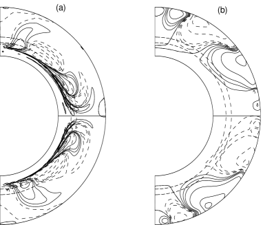
Figure 1: Toroidal (left) and poloidal (right) magnetic fields in the dynamo solution obtained with the non-local buoyancy formalism of Dikpati & Charbonneau (1999).

We plan to make our dynamo code available in the public domain, with the settings of parameters used to generate our standard solution presented in §3.1 and §4 of CNC. We are now in the process of making the code more user-friendly and preparing a guide for it. The code and the guide should be available in the public domain latest by 1 December 2005. The entire solar physics community should be able to examine our code and verify whether it produces the results presented in CNC.

3 Response to other criticisms

We now respond to the other criticisms of DRGM on the basics of our model—criticisms which do not necessarily depend on the fact that DRGM were unable to reproduce our results.

3.1 Is our dynamo model circulation-dominated?

The longest subsection of DRGM (§3.1) is devoted to questioning the name ‘circulation-dominated’ we had given to our dynamo model. Although the discussion of DRGM seems to us nothing more than mere quibbling over semantics, let us explain our point of view. We have $d\Omega/dr$ positive at the lower latitudes, and the $\alpha$ coefficient is also positive. According to the well-known dynamo sign rule (see, for example, Choudhuri 1998, §16.5), the dynamo wave should propagate poleward. Still the toroidal field below the bottom of the solar convection zone (SCZ) moves equatorward, because it is advected through a region where the diffusivity has a low value $\eta_{RZ}=2.2\times 10^{8}$ cm² s^-1 and it essentially remains frozen in the fluid. Even if we take a rather low value of $d=10^{4}$ km for the thickness of the layer below the SCZ through which the toroidal field is advected, still the diffusion time $d^{2}/\eta_{RZ}$ turns out to be about 144 yr—much larger than the time scale of advection by the meridional circulation. That is why the toroidal field simply gets advected through a thin layer below the bottom of SCZ while remaining frozen and we have felt that ‘circulation-dominated’ is the appropriate name of a dynamo model in which this happens. If DRGM do not like our name, they are free to use any other name. We are surprised that they took about one journal page to debate something which appears to us a trivial matter of semantics.

3.2 TF/PF ratios

In §3.4 of DRGM, our model is criticized on the ground that polar fields of order 2 kG are needed to generate 100 kG toroidal fields. The answer to this criticism can be found in §2–3 of an already published paper by Choudhuri (2003). DRGM’s argument is based on a serious misconception. The dynamo equation deals with the mean magnetic field. On the other hand, flux tube rise simulations suggested a magnetic field of 100 kG only inside the flux tubes—the mean field being much less if the flux is organized intermittently. Choudhuri (2003, §2) presented some straightforward back-of-the-envelope estimates showing that a circulation-dominated dynamo can stretch a polar field of 10 G to a maximum toroidal field of only about 10 kG. So the mean toroidal field can be at most of this value. The toroidal field has to be highly intermittent, with the value of 100 kG occuring only in isolated regions. This is an entirely consistent physical scenario.

3.3 Different diffusivities for PF and TF

Since there are not separate conducting fluids for toroidal and poloidal fields, DRGM argue in §4.2 that assuming different diffusivities at the same point is implausible. However, the diffusivities entering the dynamo equation are not actual ‘physical’ diffusivities, but effective turbulent diffusivities which arise from an averaging procedure and describe how the mean fields evolve. We believe that the magnetic field at the base of SCZ looks as sketched in Fig. 3 of Choudhuri (2003), with the flux concentrations stretching along the $\phi$ direction. Turbulent diffusivity is obviously suppressed within these flux concentrations, making the magnetic field $B_{\phi}$ in these regions of concentration rather immune to turbulent diffusivity. If we were doing calculations with the full magnetic field, then we could capture this effect through a simple quenching of turbulent diffusivity. But we have to average over regions much larger than the flux concentrations to get the mean field dynamo equation. How do we capture the information in the dynamo equation that diffusivity is suppressed within $B_{\phi}$ concentrations having sizes smaller than the scale of our mean field theory? We felt that taking a smaller diffusivity for $B_{\phi}$ is one way of handling this issue. We do not claim that this is a very satisfactory or mathematically rigorous way. But we have not been able to think up any better way of tackling this issue.

3.4 Penetration depth of meridional circulation

DRGM argue in §4.1 that the meridional circulation could not penetrate below the bottom of SCZ which we require. It may be pointed out that Dikpati & Charbonneau (1999) produced their best dynamo models with a deeply penetrating meridional circulation, without clearly mentioning anywhere in the text that this was essential to obtain good models. The fault of Nandy & Choudhuri (2002) seems to be that they were the first who asserted clearly that a penetrating flow is required to produce satisfactory circulation-dominated solar dynamo models and discussed its physical implications. Fig. 2 shows the radial profiles of $v_{\theta}$ at $\theta=45^{\circ}$ used by us as well as by Dikpati & Charbonneau (1999). No comment is necessary. Linguists and sociologists of science would be particlularly intrigued to note the language employed by DRGM to describe these two velocity fields. DRGM write “Dikpati & Charbonneau (1999) used an equatorward return flow which penetrated slightly below $0.7R$”, while DRGM’s comment on our velocity field is: “Nandy & Choudhuri (2002) had a subsurface return flow of about a 10 m s^-1 at $r=0.6R$”! We have no clue whatsoever how DRGM arrived at the extraordinary conclusion of our model having a velocity of 10 m s^-1 at $r=0.6R$, when a plot of velocity versus depth was given in Fig. 3 of CNC.

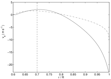
Figure 2: Plot of $v_{\theta}$ (in m s^-1) as a function of $r$ at the mid-latitude $\theta=45^{\circ}$. The solid line shows the velocity used by CNC, whereas the dashed dotted line is the velocity used by Dikpati & Charbonneau (1999; see Fig. 1c).

Defending the meridional circulation used by Dikpati & Charbonneau (1999), DRGM write: “Given the knowledge available at that time about the meridional circulation, it was reasonable to try what Dikpati & Charbonneau (1999) did, but not in 2004 …” DRGM have not clarified for the benefit of the readers whether it was still reasonable to try this in 2002 when Nandy & Choudhuri (2002) wrote their paper, although during 2001–2002 it was stated in successive dynamo papers of the HAO group (Dikpati & Gilman 2001; Dikpati et al. 2002) that they were using the same meridional circulation as Dikpati & Charbonneau (1999)! However, we are given to understand that 2004 is the decisive year when such meridional circulations ceased to be ‘reasonable’—the year marked by the publication of a paper by Gilman & Miesch (2004). We humbly beg to differ from this point of view. The bottom of the SCZ is the least understood region in the interior of the Sun. Recently one of us (A.R.C.) attended a workshop on the tachocline at Isaac Newton Institute in Cambridge, where one of the authors of the DRGM paper (P.A.G.) was also present. From the very heated discussions there, it was obvious that there is no general agreement regarding the extent of overshooting below the base of SCZ or the extent of turbulence in the tachocline. We agree with Gilman & Miesch (2004) that the meridional circulation could not penetrate much into a stable region where there is no overshooting or turbulence. However, in our current state of ignorance, we cannot rule out the possibility of enough overshooting and turbulence existing throughout the tachocline below the bottom of SCZ and a meridional circulation penetrating through this region. We cannot present detailed arguments within the three pages kindly allotted by the A&A Editor for our reply. A paper under preparation will address this issue.

4 Conclusion

To sum up, DRGM probably got results different from ours by treating the magnetic buoyancy unsatisfactorily. Their other criticisms of our model do not appear very relevant.

References

Chatterjee, P., Nandy, D., & Choudhuri, A. R. 2004, A & A, 427, 1019
Choudhuri, A. R. 1998, The Physics of Fluids and Plasmas: An Introduction for Astrophysicists (Cambridge: Cambridge University Press)
Choudhuri, A. R. 2003 Sol. Phys., 215, 31
Choudhuri, A. R., Chatterjee, P., & Nandy, D. 2004, ApJ, 615, L57
Choudhuri, A. R., & Dikpati, M. 1999, Sol. Phys., 184, 61
Choudhuri, A. R., Schüssler, M., & Dikpati, M. 1995 A & A, 303, L29
Dikpati, M., & Charbonneau, P. 1999, ApJ, 518, 508
Dikpati, M., & Choudhuri, A. R. 1995 Sol. Phys., 161, 9
Dikpati, M., Corbard, T., Thompson, M. J., & Gilman, P. A. 2002, ApJ, 575, L41
Dikpati, M., & Gilman, P. A. 2001, ApJ, 559, 428
Dikpati, M., Rempel, M., Gilman, P. A., & MacGregor, K. B. 2005, A & A, in press
Gilman, P. A., & Miesch, M. S. 2004, ApJ, 611, 568
Nandy, D., & Choudhuri, A. R. 2001, ApJ, 551, 576
Nandy, D., & Choudhuri, A. R. 2002, Science, 296, 1671