Hydrodynamical stellar models including rotation,
internal gravity waves and atomic diffusion

In this paper, we develop a formalism in order to incorporate the contribution of internal gravity waves to the transport of angular momentum and chemicals over long time-scales in stars. We show that the development of a double peaked shear layer acts as a filter for waves, and how the asymmetry of this filter produces momentum extraction from the core when it is rotating faster than the surface. Using only this filtered flux, it is possible to follow the contribution of internal waves over long (evolutionary) time-scales.

We then present the evolution of the internal rotation profile using this formalism for stars which are spun down via magnetic torquing. We show that waves tend to slow down the core, creating a “slow” front that may then propagate from the core to the surface. Further spin down of the surface leads to the formation of a new front. Finally we show how this momentum transport reduces rotational mixing in a $1.2\,M_{\odot}$, $Z=0.02$ model, leading to a surface lithium abundance in agreement with observations in the Hyades.

1 Introduction

Stellar models are getting more and more sophisticated. In order to explain detailed observed features of stars in various places of the Hertzsprung-Russell diagram, modern stellar evolution codes must indeed incorporate several complex physical processes which are often referred to as “non-standard”. The main ones are :

• Atomic diffusion (gravitational settling, thermal diffusion, radiative forces);

• Large scale mixing due to rotation (turbulence, meridional circulation);

• Convective overshooting;

• Internal gravity waves (IGW);

• Magnetic fields.

All these processes are not necessarily present at the same time everywhere in the HR diagram. Additionally they act on very different characteristic timescales in stars of various initial masses and evolutionary stages. In order to provide a coherent picture of stellar evolution, one must thus understand why some dominate in certain stellar types and not in others. Furthermore, one has to pay attention to their possible interactions and interdependence.

These mechanisms affect evolutionary tracks, lifetimes, surface abundances, chemical yields etc. Their impact on the stellar structure and evolution arises mainly from the redistribution of chemical elements that they cause, and which is related (except in the case of atomic diffusion) to the induced redistribution of angular momentum inside the stars. During the last fifteen years, many studies have been devoted to describe the evolution of the angular momentum distribution because this pattern governs the extent of rotation-induced mixing in stellar interiors. For models in which the internal rotation law evolves under the effects of meridional circulation, shear mixing, horizontal turbulence, mass loss, contraction and expansion (i.e., neglecting the transport by IGW and by magnetic fields) the main results can be summarized as follows :

• On the one hand, models which take into account the hydrodynamical processes induced by rotation as described by Zahn (1992), Maeder (1995), Talon & Zahn (1997) and Maeder & Zahn (1998) are very successful in explaining the observed “anomalies” in stars which do not have extended envelopes. Among the many successes of these models one can quote the reproduction of the left side of the Li dip in field and open cluster stars, of the constancy of the CNO abundances within the Li dip and of the evolution of Li abundance in sub-giants (Charbonnel & Talon 1999, Palacios et al. 2003, Pasquini et al.2004). For more massive stars these models explain for example the observed He and N enrichment in main sequence O- and early B-type stars, in OB super-giants and in A-type SMC super-giants. They also account for the observed variations of the Wolf-Rayet star populations as well as the fractions of type Ib/Ic supernovae with respect to type II SN at various metallicities (see Maeder & Meynet 2000, Meynet & Maeder 2005 and references therein).

• On the other hand, the same input physics fails to reproduce some of the most constraining observed features in low-mass stars which have deep convection envelope. First of all, meridional circulation and shear turbulence alone are not efficient enough to enforce the flat solar rotation profile measured by helioseismology (Brown et al. 1989; Kosovichev et al. 1997; Couvidat et al. 2003; Pinsonneault et al. 1989; Chaboyer et al. 1995 ; Matias & Zahn 1998). Additionally the rise of the Li abundance on the red side of the dip cannot be explained if one assumes that momentum is transported only by the wind-driven meridional circulation in those main-sequence stars which are efficiently spun down via magnetic torquing (Talon & Charbonnel 1998). Last but not least, the current rotating models are insufficient to explain the anomalies in C and N isotopes observed in field and cluster red giant stars (Palacios et al. 2005).

The successes and difficulties described above have revealed the occurrence of an additional process that participates in the transport of angular momentum in relatively low-mass stars which have extended convective envelopes and are spun down via magnetic braking in their early evolution (Talon & Charbonnel 1998). This process must act in conjunction with meridional circulation, turbulence and atomic diffusion. As of now, two candidates have received some attention, namely internal gravity waves and magnetic fields.

Internal gravity waves have initially been invoked as a source of mixing for chemicals (Press 1981, García López & Spruit 1991, Schatzman 1993, Montalbán 1994, Montalbán & Schatzman 1996, 2000, Young et al. 2003). Ando (1986) studied the transport of momentum associated with standing, gravity waves. He showed how momentum redistribution by these waves may increase the surface velocity to induce episodic mass-loss in Be stars. Goldreich & Nicholson (1989) used them later in order to explain the evolution of the velocity of binary stars, producing synchronization that proceeds from the surface to the core. Traveling internal gravity waves have since been invoked as an important process in the redistribution of angular momentum in single stars spun down by magnetic torquing (Schatzman 1993, Kumar & Quataert 1997, Zahn, Talon, & Matias 1997).

In a previous series of papers, we examined the generation of internal gravity waves by the surface convection zone of stars with various masses and metallicities. We found that these waves, which are able to extract angular momentum from the deep solar interior (Talon, Kumar, & Zahn 2002, hereafter TKZ), have a very peculiar mass (or more precisely effective temperature) dependence and could possibly dominate the transport of angular momentum in stars with deep enough convective envelope (Talon & Charbonnel 2003, 2004). We suggested that such a dependence could lead to a coherent picture of rotational mixing in stars of all masses at various evolution phases. It could for example explain simultaneously the cold side of the Li dip as well as the solar rotation profile and the existence of fast rotating horizontal branch stars (see Talon & Charbonnel 2004 for more details).

An important characteristic of internal waves is that, unless they are damped, they conserve their angular momentum even when their local frequency is modified by Doppler shifting. This should be kept in mind throughout the reading of this paper. For a comprehensive review of gravity wave properties, we suggest Bretherton (1969) and Zahn et al. (1997) for an application to the stellar, spherical case.

The other mechanism that has been invoked to enforce the Sun’s flat rotation profile requires a pre-existing fossil magnetic field (Charbonneau & Mac Gregor 1993; Barnes, Charbonneau, & Mac Gregor 1999). However no mass dependence is expected in that case. This is in contradiction with the Li dip constraint (although in this case this feature could be explained in purely solid body rotation by the combined action of solid body meridional circulation and radiative forces; see Charbonneau & Michaud 1988) and more importantly with the large rotational velocities measured in some horizontal branch stars.

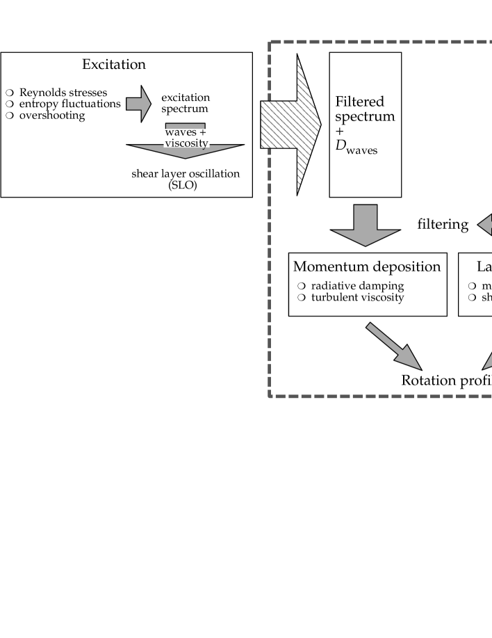
Figure 1: Schematic view of the physical processes and their interactions involved in momentum redistribution by IGW. Complete calculations take into account all processes enclosed in the dashed box.

Let us also mention calculations of massive star models by Maeder & Meynet (2003) in which the Taylor-Spruit dynamo (Spruit 1999, 2002), which is thought to be the most efficient dynamo mechanism in the radiative region, is included. When considered as is, this mechanism induces almost solid body rotation, efficiently reducing the extent of rotational mixing. It also leads to stellar models whose properties are closer to those of standard models and thus, in lesser agreement with stellar observations. When reviewing the efficiency of this mechanism by taking into account energy conservation, it is found that the dynamo is not as efficient as first thought. In fact, calculations for a $15\leavevmode\nobreak\ M_{\odot}$ star model show that adding the contribution of magnetic field only slightly modifies the results obtained with the purely hydrodynamic models (Maeder & Meynet 2004 and Maeder, private communication). Let us recall that for such massive stars with no convective envelope internal gravity waves can not be produced efficiently and thus the present rotating models would remain unchanged in our global picture.

All these results and constraints obtained for stars covering a large fraction of the HR diagram strongly incite further studies of the combined effects of rotation and internal gravity waves in stars where these waves are known to be efficiently produced. Although they do not definitively disgrace magnetic fields which certainly play a role in the complete picture, they bring sufficient arguments to justify complete tests of a fully hydrodynamical model before including MHD effects.

This is what we intend to do in the present series of papers where we will investigate the combined and sometimes conflicting effects of rotation, internal waves and atomic diffusion in low- and intermediate-mass stars at various stages of their evolution. We will present the first fully hydrodynamical stellar models that include self-consistently the chemical and momentum redistribution by these three mechanisms.

In the present paper we discuss the formalism that we will use in the hydrodynamical models which will be presented here and in forthcoming studies. A schematic view of all physical ingredients included and their interactions is shown in Fig. 1. In § 2, we first describe the prescription we follow for wave generation or excitation. Then in § 3, we come back to the properties of the shear layer oscillation (or SLO) which builds up below the surface convection zone of the star and on the momentum extraction by the waves in the radiative region. We explain how an excited wave spectrum combined with the action of the SLO may be replaced by a filtered spectrum and a diffusion coefficient, as illustrated in Fig. 1. General equations for the transport of angular momentum and chemicals are written in the global scheme (§ 4 and 5), which takes into account momentum deposition beyond the shear layer and momentum transport by meridional circulation and shear turbulence. Then we recall some properties of the transport by waves using a static model (§ 6). Finally we present the first results for a $1.2\,M_{\odot}$, $Z=0.02$ star computed within the complete physical framework (§ 7) before concluding (§ 8).

2 Internal Gravity Wave Generation

Gravity waves are produced, among other things, by the injection of kinetic energy from a turbulent region to an adjacent stable region. This is observed for example at the border of clouds in the earth’s atmosphere (Townsend 1965) and also in laboratory experiments (Townsend 1958). It should also occur in stars. This was already illustrated in the early (2D) numerical simulations of convection including penetration by Hurlburt et al. (1986, see also Hurlburt et al. 1994, Andersen 1994, Nordlund et al. 1996, Kiraga et al. 2000, Rogers & Glatzmeier 2005). There are two ways to excite those waves:

• convective overshooting in a stable region;

• bulk excitation, similar to that of the solar pressure waves.

Excitation by overshooting is probably the most difficult to evaluate analytically. The first attempt was made by García López & Spruit (1991) by assuming that the pressure perturbation produced by turbulent eddies at the radiative/convective boundary is equal to the wave pressure perturbation. In this model, stochastic eddies of a given size are considered to contribute to the excitation of a whole wavelength spectrum. As formulated, this model rests on the assumption of homogeneous turbulence, although it could be modified to incorporate the presence of downdrafts observed in numerical simulations of convection. Another estimate for this process has been made by Fritts, Vadas, & Andreassen (1998), in a study aimed at estimating the residual circulation induced by latitude dependent dissipation in the tachocline. However, they concentrate on the small wavelength waves that dissipate close to the convection zone and their mechanism does not take into account the combination of small scale eddies in order to produce low degree waves. Such waves are essential in order to influence the inner layer on an evolutionary time-scale (TKZ). Let us also mention here that the results presented in this study depend on the latitudinal differential rotation and cannot (as of now) be generalized to stars other than the Sun.

Kiraga et al. (2003) tried to evaluate the validity of the García López & Spruit approach by comparing the predictions of this model to a simulation of penetrative convection. The peak wave spectrum produced by the simulation was similar in amplitude to that of this parametric model. However, in the simulation modes where excited over a much broader range of frequencies and wavelengths. It is not clear whether this is related to the bi-dimensional nature of the simulation of to shortcomings of the model.

Internal gravity waves can also be excited in the convection zone itself. In that region, modes are evanescent and their amplitude is proportional to $\exp\left[-\int{\rm d}r\,k_{r}\right]$, where $k_{r}$ is the radial wave number. Press (1981) used the formalism of Goldreich & Keeley (1977) to show that Reynolds-stress and buoyancy may excite gravity waves with a rather large amplitude at the bottom of the convection zone. Goldreich & Kumar (1990) and Goldreich, Murray, & Kumar (1994, GMK) completed the Goldreich & Keeley formalism in order to apply it to solar p-modes. Their model quite successfully reproduces the solar spectral energy input rate distribution, provided one free parameter which describes the geometry of turbulent eddies is calibrated. In that case, driving is dominated by entropy fluctuations. Balmforth (1992) made a similar study, using a somewhat different formalism. Subject to the calibration of a free parameter, he is also able to reproduce the spectral energy distribution; however, it is the Reynolds-stress that is the main source of driving.

Figure 2: Penetration of IGW into the convection zone of a ZAMS $1\,M_{\odot}$ model for various degrees $\ell$. The arrows indicate the depth where the amplitude is reduced by a factor of 2. Also shown is the local convective flux given by the mixing length theory.

In the present study, we follow Kumar & Quataert (1997) and apply the GMK formalism to traveling internal gravity waves. This was also used by Kumar, Talon, & Zahn (1999), TKZ, Talon & Charbonnel (2003, 2004). The energy flux per unit frequency ${\cal F}_{E}$ is then

$${\cal F}_{E}\left(\ell,\omega\right) = \frac{\omega^{2}}{4\pi}\int dr\;\frac{\rho^{2}}{r^{2}}\left[\left(\frac{\partial\xi_{r}}{\partial r}\right)^{2}+\ell(\ell+1)\left(\frac{\partial\xi_{h}}{\partial r}\right)^{2}\right]$$ (1)

$$\times\exp\left[-h_{\omega}^{2}\ell(\ell+1)/2r^{2}\right]\frac{v^{3}L^{4}}{1+(\omega\tau_{L})^{15/2}},$$

where $\xi_{r}$ and $[\ell(\ell+1)]^{1/2}\xi_{h}$ are the radial and horizontal displacement wave-functions which are normalized to unit energy flux just below the convection zone, $v$ is the convective velocity, $L$ is the radial size of an energy bearing turbulent eddy, $\tau_{L}\approx L/v$ is the characteristic convective time, and $h_{\omega}$ is the radial size of the largest eddy at depth $r$ with characteristic frequency of $\omega$ or greater ($h_{\omega}=L\min\{1,(2\omega\tau_{L})^{-3/2}\}$). The radial wave number is related to the horizontal wave number $k_{h}$ by

$$k_{r}^{2}=\left(\frac{N^{2}}{\sigma^{2}}-1\right)k_{h}^{2}=\left(\frac{N^{2}}{\sigma^{2}}-1\right)\frac{\ell\left(\ell+1\right)}{r^{2}}$$ (2)

where $N^{2}$ is the Brunt-Väisälä frequency. In the convection zone, the mode is evanescent and the penetration depth varies as $\sqrt{\ell\left(\ell+1\right)}$. Figure 2 compares this distance for various modes with the convective energy that is locally available. In the outer part of the model, the luminosity is carried almost uniquely by convection.

The momentum flux per unit frequency ${\cal F}_{J}$ is then related to the energy flux by

$${{\cal F}_{J}}\left(m,\ell,\omega\right)=\frac{m}{\omega}{\cal F}_{E}\left(\ell,\omega\right)$$ (3)

(Goldreich & Nicholson 1989, Zahn et al. 1997).

3 Evolution of Angular Momentum

Figure 3: Behavior of the shear layer as a function of the diminishing viscosity for a $1.3\,M_{\odot}$ model with a turbulent viscosity given by Eq. (4). From left to right, $N=8$, $N=7.9$ and $N=7.85$. (top) Time evolution of the rotation velocity at two different depths. (Full line) $\Omega(r_{1})$ (dashed line) $\Omega(r_{2})$ with $r_{1}=r_{cz}-0.003H_{P}$ and $r_{2}=r_{cz}-0.015H_{P}$. (bottom) Phase space diagram.

3.1 Wave Mean-Flow Interaction and the SLO

It is now well established that the dissipation of internal gravity waves in a differentially rotating region leads to an increase in the local differential rotation. In stellar models, this leads to the formation of a narrow ($\sim$ 1-2% in radius) doubled peak oscillating shear layer adjacent to the convection zone where they are produced (Gough & McIntyre 1998, Ringot 1998, Kumar, Talon, & Zahn 1999). We shall refer to this process as “shear layer oscillation” or SLO.

In a simple two waves model, Kim & MacGregor (2001) examined the behavior of that layer, which depends on the ratio between viscosity and wave flux. If the viscosity is large, a stationary solution may be found. There then exists a bifurcation to an oscillatory behavior of the shear as viscosity is reduced. Further reduction leads to the appearance of chaos. The determination of the stellar viscosity is thus of key importance for the structure of this layer.

If only radiative viscosity is considered, one observes the formation of a very steep and narrow shear layer, and chaotic behavior is expected. However, as the local shear increases, it may lead to the appearance of a shear instability, which will enhance the local viscosity compared to its microscopic value. This process actually self-regulates the wave-mean flow interaction. Indeed, a larger wave flux leads to a larger differential rotation which in turns acts as to increase the local viscosity.

Several calculations have been performed, using various prescriptions for the turbulent viscosity. The first case-study should consist of using simply the radiative viscosity. It has the major advantage that it can be derived from first principles only. However, this viscosity is so low compared to the wave flux that it rapidly leads to a slow layer that is stopped and even begins to rotate backward. To prevent that, we will consider a “turbulent” viscosity proportional to the radiative viscosity

$$\nu=10^{N}\nu_{\rm rad}.$$ (4)

A regular oscillating layer is formed for $N=8$ (a similar form was used by TKZ). For a slightly larger ($N=9$) viscosity, we no longer obtain an oscillation. This corresponds to the stationary solution found by Kim & MacGregor (2003). Here, we do not find a stationary profile due to the use of different boundary conditions (Neumann rather than Dirichlet); our solution slowly decays to a state of solid body rotation. For smaller ($N=7.9$ and $N=7.85$) viscosities, there is a transition to chaos. These results generalize the Kim & MacGregor (2001) results to the case where a complete wave spectrum is considered. Period doubling is not readily identified in this simulation. Figure 3 summarizes our findings.

The turbulent viscosities used so far are not realistic. They vary only slowly with depth, and remain large even far from regions where there exists a physical mechanism to produce this turbulence. We must thus find a reliable prescription in order to estimate the magnitude of turbulence on physical grounds.

The structure of the shear region points to the shear instability as an important source of turbulence. Generally, its magnitude depends on the local shear rate and on the efficiency of buoyancy which acts as a restoring force. When taking into account radiative losses (Townsend 1958, Dudis 1974, Lignières et al. 1999) and the effect of horizontal turbulence on the stabilizing effect of mean molecular weight gradients (Talon & Zahn 1997), the viscous turbulence may be approximated by

$$\nu_{v}=\frac{8}{5}\frac{Ri_{\rm crit}(r{\rm d}\Omega/{\rm d}r)^{2}}{N^{2}_{T}/(K+D_{h})+N^{2}_{\mu}/D_{h}}.$$ (5)

This formulation is based on the local shear rate. In a rapidly varying profile, such as the one we get in the shear layer, it leads to large gradients in the turbulent diffusion coefficient, and is probably not realistic. Indeed, vertical turbulence can develop over vertical scales similar to the pressure scale height which is greater than the scale of the variations of the shear layer (less than $1$% in radius, see e.g. Fig. 4, while in low mass main sequence stars the pressure scale height just below the convection zone ranges from about $\sim\,10$% in radius in a $1\,M_{\odot}$ star to $\sim\,3$% in a $1.4\,M_{\odot}$ star). In practice, we thus used a convolution of the local shear turbulence given by Eq. (5) with a Gaussian of width $0.2\leavevmode\nobreak\ H_{P}$ ($H_{P}$ is the pressure scale height) in order to obtain a more realistic turbulent coefficient. Turbulence is also averaged over a complete oscillation cycle.

Figure 4: (left) Shear layer evolution (successive profiles are separated by 1 year) and (right) average turbulent viscosity (as described in § 3.1). The dashed line corresponds to an analytical fit (cf. Eq. 17).

Figure 5: Wave characteristics below the shear layer for a differential rotation of $\delta\Omega=0.1\leavevmode\nobreak\ \mu{\rm Hz}$ over $5\%$ in radius in a 1.3 $M_{\odot}$ star. First and second row: Wave amplitude for $m=\pm 1$ and $m=\pm\ell$. Third row: Amplitude difference between retrograde and prograde waves of the same azimuthal number. Fourth row: Net luminosity for a given azimuthal number.

In this framework, the magnitude of the shear layer is self-regulated. An increase in the wave flux leads to an increased differential rotation and thus, an increase of the shear turbulence.

Calculations are shown here for a $1.3\,M_{\odot}$, $Z=0.02$ model. Figure 4 shows the evolution of the shear layer as well as the self-consistent turbulent viscosity induced in the model. In this model, thermal diffusion is rather large (see Talon & Charbonnel 2003). This explains the large value for the turbulent coefficient, and also its extreme thinness. In lower mass stars, while just below the convection zone the viscosity is large enough to lead to a regular oscillating layer, it then decreases rapidly in the interior, leading to a complex layer structure that has a chaotic behavior. However, this has no particular impact on long term momentum extraction.

This turbulence is generated by wave momentum deposition due to radiative damping, and is related to turbulence produced by large amplitude waves where they are dissipated (Press 1981, Canuto 2002, Young et al. 2003). It is quite different in essence from the turbulent diffusion generally associated with waves, either due to wave breaking (Press 1981, García López & Spruit 1991) or to irreversible second order motions (Press 1981, Schatzman 1993, Montalbán 1994). This issue will be discussed further in § 5.

3.2 Momentum Deposition Beyond the Shear Layer

The superficial shear layer acts as a filter on internal gravity waves (Gough & McIntyre 1998). Indeed, as internal waves travel across first a “rapid” and then a “slow” layer, prograde and retrograde waves respectively are preferentially damped. However, some of the power remains in the lowest order waves, and over long time-scales (of the order of evolutionary time-scales), momentum redistribution below the shear layer cannot be neglected (TKZ). Figure 5 illustrates wave characteristics below the shear layer for a given differential rotation, with the convection zone rotating slower than the radiative zone. The two top rows compare the amplitude of retrograde and prograde waves. As shown in the third panel, the retrograde waves are somewhat less damped then their prograde counterparts, and this leads to a net luminosity of momentum, illustrated in the bottom panel. As explained in TKZ this is because the underlying differential rotation produces a prograde layer which, on average, is always larger than the retrograde layer.

It is the low frequency, low degree waves that give the largest contribution to momentum redistribution in the interior; high degree waves are damped closer to the convection zone (as damping $\propto\ell\left(\ell+1\right)^{3/2}$) and thus have an intrinsically small amplitude below the shear layer while high frequency waves experience less differential damping ($\propto 1/\sigma(r)^{4}=1/\left[\omega-m\left(\Omega(r)-\Omega_{\rm cz}\right)\right]^{4}$), crucial to produce a net momentum deposition (see Fig. 6). See § 4 for details on damping.

In order to built evolutionary stellar models, it is not possible to follow in detail the behavior of the oscillating shear layer, which occurs on time-scales of years or tens of years. However, this shear layer is crucial in filtering the low order waves that travel through it. The net wave flux across the shear layer depends of the asymmetry of the filter and thus, on the difference between the rotation velocity below the shear layer and that of the convection zone. Let us note however that the thickness of the oscillating layer is independent of this asymmetry. Last but not least, wave momentum transport does not have a diffusive behavior and as such must not be treated merely as a turbulent diffusion process.

Figure 6 illustrates differential damping in a shear region, with both a “rapid” and a “slow” layer. The $m=0$ mode is not affected by the differential rotation, and, for a given frequency, the damping length $\delta$ is inversely proportional to $\ell(\ell+1)$. The “rapid” layer increases the damping of prograde modes, and reduces it for the retrograde modes. The reverse is obtained from the “slow” layer.

Figure 6: (top) Instantaneous rotation profile (middle, bottom) Instantaneous damping length (corresponding to a reduction of wave amplitude $A=A_{0}/e$) for wave frequencies of $\nu=0.5$ and $\nu=1\leavevmode\nobreak\ \mu{\rm Hz}$ in a 1.3 $M_{\odot}$ star. The $m=0$ mode (open dots) is not affected by rotation, the $m=\pm\ell$ (squares and triangles) are the most affected. Below the shear layer, the radiative region is rotating more rapidly; it is the retrograde modes of low order that penetrate deeper, leading to a net deposition of negative momentum in the interior. The low ($\ell=1$ and $2$) modes have to travel back and forth a few times before they are damped, and are not shown in the bottom graph.

Figure 7: Local deposition of angular momentum for various values of differential rotation. The rotation profile rises linearly between the base of the convection zone and $(1-m/M)=-2.85$ by a value of $\delta\Omega$, which varies logarithmically from $10^{-5}$ to $10^{-1}$ $\mu{\rm Hz}$. This is illustrated for a $1.3\,M_{\odot}$ model. For moderate amounts of differential rotation (below $\sim\leavevmode\nobreak\ 10^{-2}\leavevmode\nobreak\ \mu{\rm Hz}$), the net momentum flux at a given point is a linear function of differential rotation.

Figure 7 shows the local momentum deposition for various values of differential rotation. As far as differential rotation is not too large, momentum deposition varies linearly with $\delta\Omega$. Actual calculations of the evolution of the distribution of angular momentum show that, for realistic values of braking (according to Kawaler 1988), the star remains in this linear regime.

3.3 Energy Considerations

It has been shown elsewhere (Kumar & Quataert 1997, Zahn et al. 1997, TKZ) that gravity waves can carry enough angular momentum to slow down the radiative zone of low mass stars on time-scales of order $10^{7}$ years. One may wonder however if the deposition of energy by waves may have an impact on the stellar structure. Let us first begin by comparing the amount of energy contained in gravity waves with other quantities. This will be done here for a ZAMS $1\,M_{\odot}$ model.

The total energy luminosity in waves is of order $10^{29}\leavevmode\nobreak\ {\rm ergs\,s^{-1}}$, while the total luminosity at the base of the convection zone is $2.5\times 10^{33}\leavevmode\nobreak\ {\rm ergs\,s^{-1}}$, of which a large part is convective (see Fig. 2). The wave luminosity thus represents about $0.01$% of the convective luminosity.

Let us next look at the amount of kinetic energy that is stored in rotation $K_{\Omega}$. We have $K_{\Omega}=\frac{1}{2}I\Omega^{2}$ with $I$ the moment of inertia of the star. For the whole star, it is of order $10^{54}\leavevmode\nobreak\ {\rm cm^{2}\,g}$. For an initial rotation velocity of $100\leavevmode\nobreak\ {\rm km\,s^{-1}}$, this leads to an energy of $10^{46}\leavevmode\nobreak\ {\rm ergs}$. As the star is spun down, this energy must be dissipated and will be added to the thermal energy. However, the total rotation energy is two order of magnitude lower than the thermal content and so, the impact will be negligible on the stellar structure.

4 A Model for Angular Momentum Evolution by Waves

Gravity waves lead to two different features that must be incorporated in stellar evolution codes:

• They produce a shear layer, that generates turbulence close to the bottom of the convection zone;

• They deposit negative (positive) momentum throughout the radiative interior when the convection zone rotates slower (faster) than the radiative zone.

The turbulent region is always present, and the shear layer oscillation is (almost) independent of the presence or absence of differential rotation below. The magnitude of the turbulence and the size of the turbulent region are self-regulated and depend on the wave flux. For a given wave-excitation model, and a given model for the turbulent diffusion, we obtain a localized turbulent region.

The net momentum luminosity spectrum below the shear layer for various masses is shown in Fig. 8. To obtain the net momentum deposition, one must follow the local momentum luminosity

$${\cal L}_{J}(r)=\sum_{\sigma,\ell,m}{{\cal L}_{J}}_{\ell,m}\left(r_{\rm shear\leavevmode\nobreak\ layer}\right)\exp\left[-\tau(r,\sigma,\ell)\right]$$ (6)

and where the local damping rate takes into account the mean molecular weight stratification

$$\tau(r,\sigma,\ell)=[\ell(\ell+1)]^{3\over 2}\int_{r}^{r_{c}}\left(K+\nu_{t}\right)\;{NN_{T}^{2}\over\sigma^{4}}\left({N^{2}\over N^{2}-\sigma^{2}}\right)^{1\over 2}{{\rm d}r\over r^{3}}$$ (7)

where $N^{2}=N_{T}^{2}+N_{\mu}^{2}$ is the total Brunt-Väisälä frequency, $N_{T}^{2}$ is its thermal part and $N_{\mu}^{2}$ is due to the mean molecular weight stratification (cf. Zahn et al. 1997). $\sigma$ is the local, Doppler shifted frequency

$$\sigma(r)=\omega-m\left(\Omega(r)-\Omega_{\rm cz}\right)$$ (8)

and $\omega$ is the wave frequency in the reference frame of the convection zone. Only those waves with a sufficient amplitude after filtering have to be traced.

When meridional circulation, turbulence and waves are taken into account, the evolution of angular momentum thus follows

$$\rho\frac{{\rm d}}{{\rm d}t}\left[r^{2}{\Omega}\right] = \frac{1}{5r^{2}}\frac{\partial}{\partial r}\left[\rho r^{4}\Omega U\right]+\frac{1}{r^{2}}\frac{\partial}{\partial r}\left[\rho(\nu_{t}+\nu_{\rm waves})r^{4}\frac{\partial\Omega}{\partial r}\right]$$ (9)

$$-\frac{3}{8\pi}\frac{1}{r^{2}}\frac{\partial}{\partial r}{{\cal L}_{J}(r)},$$

here $\rho$ is the density, $U$ the radial meridional circulation velocity, $\nu_{t}$ the turbulent viscosity due to differential rotation away from the shear layer, and $\nu_{\rm waves}$ the diffusion coefficient associated with wave-induced turbulence (see Eq. 17 in § 7.1). Horizontal averaging has been performed for this equation, and meridional circulation is considered only at first order (see § 7.1).

Figure 8: Filtered momentum luminosity spectrum for the $m=\ell$ mode (that is ${\cal L}_{\rm net}={\cal L}_{m=-\ell}-{\cal L}_{m=\ell}$) below the shear layer for various masses. Differential rotation is $\delta\Omega=10^{-4}\leavevmode\nobreak\ \mu{\rm Hz}$ over $5\%$ in radius.

5 Evolution of Chemicals

In most hydrodynamical models, chemicals evolve under the action of meridional circulation, turbulence and atomic diffusion. All these topics are discussed elsewhere (see e.g. Talon 2004 and references therein for a discussion of rotational mixing, and Turcotte et al. 1998 and references therein for a review of microscopic diffusion processes). However, when including gravity waves in momentum transport, one must also include their direct contribution to the transport of chemical species. This subject has received attention from several authors and we will here describe the main mechanisms involved.

The first process we shall discuss here is the turbulence generated in the shear layer by the shear instability. In a first step, energy is transfered by waves from the convection zone to the shear layer and stored into differential rotation, which can then be converted to turbulence by the shear instability. This view is similar to the idea of Canuto (2002) that gravity waves act as a source term in the equation that describes turbulence. This is also similar to the mixing described by Young et al. (2003). In our framework, turbulent diffusion is evaluated by taking the average of Eq. (5) over several SLO.

Weak mixing can also be induced by second order mass-transport effects in a diffusive medium (Press 1981, Schatzman 1993, Montalbán 1994). A diffusion coefficient can then be associated with wave dissipation by combining the average wave velocity and the average damping length of waves. If the concomitant transport of angular momentum is taken into account, the damping length of waves is reduced and the effect is to somewhat lower the size of the region over which this process is efficient. The thickness of the shear layer should, in many instances replace the damping length calculated in the case of solid body rotation. Differential rotation thus reduces the extent of this effect; its magnitude is at maximum of the same order as turbulence induced by the SLO. Considering the uncertainties in waves fluxes as well as on the mixing induced by those motions we suggest to neglect this effect altogether.

Finally, in certain circumstances, wave amplitude can rise to the point of becoming non-linear and inducing shear-mixing (Press 1981, García López & Spruit 1991). The non-linearity is given by

$$\epsilon\equiv k_{h}\xi_{h}=\frac{k_{h}u_{h}}{\sigma}$$ (10)

(Press 1981). The wave becomes non-linear when this parameter is of order 1 or more. In terms of energy luminosity, it is given by

$$\epsilon=\frac{k_{h}}{\sigma}\left(\frac{{\cal L}_{J}\left(r,\sigma,\ell\right)}{4\pi\rho r^{2}}\frac{k_{h}}{\left(N^{2}-\sigma^{2}\right)^{1/2}}\right)^{1/2}.$$ (11)

As estimated by Press (1981), some waves are slightly non-linear just below the convection zone; this non-linearity remains only over one damping length. However, since this region is already highly turbulent, this small non-linearity does not greatly modifies wave damping. Close to wave turning points (where $\sigma\rightarrow 0$) however, non-linearity may again become important. This will affect mostly low degree, low frequency waves by increasing their damping in that region. However, since radiative damping is already strong there, it will not greatly modify wave amplitudes. However, in some cases it could increase the amount of mixing of chemicals. García López & Spruit (1991) showed this has a significant effect only in a small part of the HR diagram (namely in stars close to the Li dip for a specific choice of the mixing length parameter). We will discuss the relevance of this effect in a future paper, where models of various masses will be implemented.

6 Waves in a Static Model

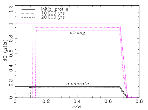
Figure 9: Evolution of the rotation profile in the case of very strong and moderate initial differential rotation in a $1\leavevmode\nobreak\ M_{\odot}$ star.

Before we apply our filtered wave model to an evolutionary calculation, let us begin by discussing some more the results obtained by TKZ in the case of a static model. Those are based on a rather small differential rotation, and use a given wave spectrum. It is worth verifying how sensitive are those results to other initial profiles or different distributions of energy. In the models presented in this section, we show results obtained for small time steps (of 1 year, as in TKZ), following the details of the shear layer oscillation. The only other process for momentum transport that is considered here is shear turbulence, and no surface braking is applied. Contrary to the TKZ study, here turbulence is directly related to the local shear rate (cf. Eq. 5).

6.1 Strong Initial Differential Rotation

Let us discuss some more results presented in § 3.2. In Fig. 9, we compare the evolution of the rotation profile in cases of very strong and moderate differential rotation. Momentum extraction from the core is clearly visible in both case. The core’s slow rotation slowly propagates toward the surface. It does so with a velocity that gets smaller as the front progresses to a region where the local angular momentum ($\propto r^{2}$) is larger. Differential rotation at the core boundary remains larger than in TKZ because the local turbulence $\nu_{t}$ is smaller. The important point to note is that in the presence of a large differential rotation, the local frequency of retrograde waves becomes very large and their damping is largely reduced in the inner regions. However, once the core has been spun down which is easily done since it contains very little momentum, a “slow” front can propagate toward the surface.

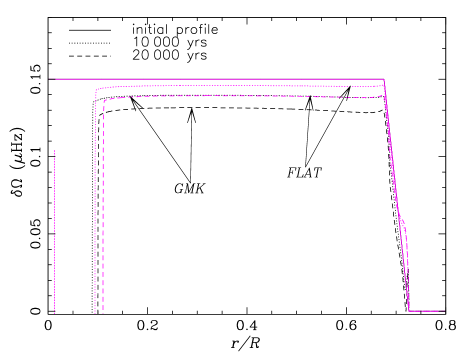
Figure 10: Evolution of the rotation profile with moderate initial differential rotation for a wave spectrum derived from GMK spectrum (cf. Eq. 1) and for a flat spectrum with the same total energy flux. Calculations are made in a $1\leavevmode\nobreak\ M_{\odot}$ star

6.2 Wave Spectrum

Another delicate point is the form of the wave spectrum. As already mentioned (§ 2), the exact spectrum produced by turbulence in the convection zone is not well constrained, and various analytical and numerical studies lead to different prescriptions. It is thus important to understand how modifying the spectrum influences the results. Figure 10 illustrates this comparison. The flat spectrum produces a front that migrates somewhat faster, but deposits less momentum in the intermediate region. In that case, the shear layer does not oscillate, but still produces a filter that preferentially damps prograde waves. While the exact spectrum changes the results quantitatively, qualitatively global effects are similar.

7 Waves in an Evolutionary $1.2\,M_{\odot}$ Model

7.1 Code Description

General inputs for stellar physics
Stellar models are computed with the stellar evolution code STAREVOL (Forestini 1991; Siess et al. 1997, 2000; Palacios et al. 2003). Our equation of state follows the Pols et al. (1995) formalism. Thermodynamical features of each plasma component (ions, electrons, photons and $\mathrm{H}_{2}$) are obtained by minimizing the Helmholtz free energy that includes separately non-ideal effects, and allows to treat ionization analytically, leading to smooth profiles for thermodynamical quantities. Radiative opacities are taken from Alexander & Fergusson (1994) below 8000 K and from Iglesias & Rogers (1996) at higher temperatures. Our nuclear reaction network follows 53 species (from ${}^{1}\mathrm{H}$ to ${}^{37}\mathrm{Cl}$) through 180 reactions. Nuclear reaction rates have been updated with the NACRE compilation (Angulo et al. 1999). Convection is treated according to the mixing length formalism with $\alpha_{p}=l/H_{p}=1.75$. No overshooting is considered.

Rotation
We follow the evolution of the rotation profile from the zero age main sequence on, assuming initial solid body rotation. The surface rotation velocity on the ZAMS is taken equal to $50\leavevmode\nobreak\ {\rm km\,s^{-1}}$. Surface spin-down follows Kawaler (1988) including saturation at $\Omega_{\rm sat}=1.5\times 10^{-5}\leavevmode\nobreak\ {\rm rad\,s^{-1}}$ (or $v\sim 10\leavevmode\nobreak\ {\rm km\,s^{-1}}$)

$$\frac{{\rm d}J}{{\rm d}t}=\left\{\begin{array}[]{l l }-K_{S}\Omega^{3}\left({\displaystyle{R}/{R_{\odot}}}\right)^{1/2}\left({\displaystyle{M}/{M_{\odot}}}\right)^{-1/2}&(\Omega\leq\Omega_{\rm sat})\\ &\\ -K_{S}\Omega\,{\Omega^{2}}_{\rm sat}\left({\displaystyle{R}/{R_{\odot}}}\right)^{1/2}\left({\displaystyle{M}/{M_{\odot}}}\right)^{-1/2}&(\Omega>\Omega_{\rm sat}).\end{array}\right.$$ (12)

The issue of saturation in the context of meridional circulation is discussed at length in Palacios et al. (2003).

IGW
To incorporate IGW, we first calculate filtered luminosities (cf. Fig. 8) for fixed differential rotations ($\delta\Omega=10^{-4},\leavevmode\nobreak\ 10^{-3},\leavevmode\nobreak\ 10^{-2}\leavevmode\nobreak\ {\rm and}\leavevmode\nobreak\ 10^{-1}\leavevmode\nobreak\ \mu{\rm Hz}$) in static ZAMS models. The wave luminosity below the surface convection zone is then linearly interpolated from those tables for the actual differential rotation just below the shear layer. The local momentum luminosity is obtained by calculating the damping integral for each individual wave (cf. Eq. 7) and then summing over all waves (cf. Eq. 6).

Meridional circulation
Meridional circulation is treated as an advection process for the transport of angular momentum, assuming strong horizontal turbulence and follows Zahn (1992).

Turbulence and diffusion
Turbulence is assumed to be strongly anisotropic, and everywhere we will assume that turbulent diffusion is equal to the turbulent viscosity. The vertical component of the turbulent viscosity

$$D_{v}=\nu_{v}=\frac{8}{5}\frac{Ri_{\rm crit}(r{\rm d}\Omega/{\rm d}r)^{2}}{N^{2}_{T}/(K+D_{h})+N^{2}_{\mu}/D_{h}}$$ (13)

takes into account the weakening effect of thermal diffusivity ($K$) on the thermal stratification and of horizontal turbulence ($D_{h}$) on both the thermal and mean molecular weight stratifications (Talon & Zahn 1997).

Horizontal turbulence follows Zahn (1992)

$$D_{h}=\nu_{h}=\frac{r}{C_{h}}\left|\frac{1}{3\rho r}\frac{{\rm d}(\rho r^{2}U)}{{\rm d}r}-\frac{U}{2}\frac{{\rm d}\ln r^{2}\Omega}{{\rm d}\ln r}\right|.$$ (14)

with $C_{h}=1$. The evolution of momentum is then given by Eq. (9).

Transport of chemicals
For chemicals, the combination of meridional circulation and horizontal turbulence results in a vertical effective diffusion

$$D_{\rm eff}=\frac{\left|rU(r)\right|^{2}}{30\,D_{h}}$$ (15)

(Chaboyer & Zahn, 1992).

Atomic diffusion driven by gravitational settling and thermal gradients is included using the formulation of Paquette et al. (1986).

The evolution of an element $c_{i}$ then follows

$$\rho\frac{{\rm d}{c_{i}}}{{\rm d}t}=\dot{c_{i}}+\frac{1}{r^{2}}\frac{\partial}{\partial r}\left[r^{2}\rho\left\{U_{ip}{c_{i}}+\left(D_{\rm eff}+D_{v}+D_{\rm waves}\right)\frac{\partial{c_{i}}}{\partial r}\right\}\right]$$ (16)

with $c_{i}$ the nuclear production/destruction rate and $U_{ip}$ the microscopic diffusion velocity with respect to protons.

Wave induced turbulence is treated explicitly through coefficient $D_{\rm waves}$ that we assume equal to the coefficient $\nu_{\rm waves}$ which enters Eq. 9. To evaluate this coefficient, we perform a time average of the diffusion coefficient associated with the local shear instability (Eq. 13) over several SLOs (see Fig. 4, and § 3.1). For evolutionary calculations, we use an analytical fit to this curve. In this application to a $1.2\leavevmode\nobreak\ M_{\odot}$ star, we used

$$\log D_{\rm waves}=\left(\log K+2\log L-68\right)\exp\left[\left(r_{\rm cz}-r\right)^{3}/\sigma\right]$$ (17)

with

$$\sigma=0.0003\left(1-r_{\rm cz}\right).$$ (18)

This fit is compared to the time-average in Fig. 4. Let us remark that above $\sim 10^{8}\leavevmode\nobreak\ {\rm cm^{2}\,s^{-1}}$, mixing may be considered “instantaneous” compared with evolutionary time-scales and thus, our analytical fit is aimed at reproducing the numerical turbulent viscosity below this value.

7.2 Evolution of the Rotation Profile

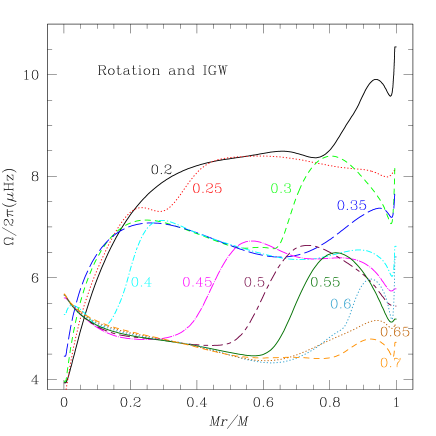
Figure 11: Evolution of the rotation profile in a complete model where the transport of angular momentum is due to internal gravity waves, meridional circulation and turbulence. The model shown is for a $1.2\,M_{\odot}$ $Z=0.02$, star with an initial rotation velocity of $50\leavevmode\nobreak\ {\rm km\,s^{-1}}$. The curves are labeled according to the corresponding ages in Gyr.

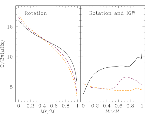
Figure 12: Same as Fig. 11 for 0.2, 0.5 and 0.7 Gyr in a case without (left) and with (right) internal gravity waves included. The time sequence goes from the highest to the smallest surface velocity

Let us first concentrate on the evolution of the rotation profile when momentum deposition by IGW is taken into account in conjunction with shear turbulence and meridional circulation. Here, the short time-scale SLO is present only as a filter; the magnitude of the wave flux depends on the amount of differential rotation between the base of the convection zone and a region just below the SLO (see § 3.2). In quasi-solid body rotation (with the surface rotating slightly slower because of braking), low degree waves penetrate all the way to the stellar core, and are damped (and thus deposit their negative momentum) over the whole radiative region. However, since the amount of angular momentum contained in the radiative core is minute, the local deposition of even a small amount of momentum is enough to spin it down significantly. In a “slow” region, damping of retrograde waves increases (cf. Eqs. 7 and 8), and this leads to the formation of a “front”, which propagates from the core to the surface. The propagation of a first front is seen in Fig. 11 (curves at 0.2, 0.25, 0.3 and 0.35 Gyr). A second front evolves from 0.4 to the 0.7 Gyr curves.

At the age of the Hyades, differential rotation is considerably reduced. In particular, it is of interest to compare calculations including and not including waves. In the second case (left plot in Fig. 12), the amount of differential rotation at the age of the Hyades is very large. This is in in agreement with the results obtained in the solar case by Matias & Zahn (1998) who performed calculations under the same hypothesis as here, and by Chaboyer et al. (1995) who approximated meridional circulation as a diffusive process.

The present complete model confirms the ability of gravity waves to efficiently extract angular momentum from the deep interior of solar-type stars. It shows how the momentum redistribution proceeds when the stars are spun down via magnetic torquing.

Let us see now what are the consequences on meridional circulation and shear turbulence, and on the Li depletion due to rotational mixing.

7.3 Meridional Circulation Velocity and Diffusion Coefficients

Figure 13 presents profiles of the vertical component of the meridional velocity $U$ at 0.5 Gyr in the $1.2\leavevmode\nobreak\ M_{\odot}$ models with and without gravity waves. When not including waves, there are two circulation loops. The meridional velocity is negative in the external part of the radiative zone down to $\sim 0.3\,M_{*}$. This meridian loop brings matter upward at the equator and down in the polar regions, in response to the extraction of angular momentum due to braking. Deeper the circulation is positive (bold line), indicating an inward transport of angular momentum. When internal waves are taken into account, several loops of circulation appear, with negative and positive loops (light and bold lines respectively) alternating.

These differences reflect directly in the transport coefficients which are shown at the same age (0.5 Gyr) in Figs. 14 and 15. Details in the profiles vary with time but this is a typical illustration. Strong variations (i.e. peaks and gaps) in the profiles of both effective and total diffusion coefficients reflect the presence of several circulation loops, each drop corresponding to an inversion of the flow direction. When gravity waves are included, the amplitude of these coefficients is reduced and vertical turbulence ($D_{v}$) is less developed than in the pure rotating models because of the decrease of the overall differential rotation.

In Fig. 15, the wave-induced turbulence ($D_{\rm waves}$) used in the present simulation with IGW and given by Eq. 17 is also shown. As can be seen, this coefficient drops very rapidly below the convection envelope and is much smaller than the total diffusion coefficient coming from rotation except very close from the convection region.

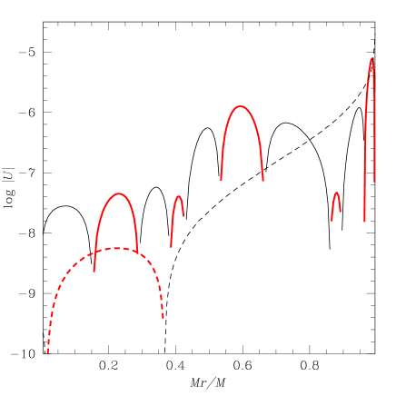
Figure 13: Profiles of the vertical component of the meridional velocity in a $1.2\,M_{\odot}$ star at 0.5 Gyr in a simple rotating model (dotted line) and in a rotating model including gravity waves (full line). The bold lines indicate positive values of $U$.

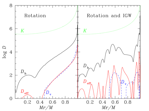
Figure 14: Comparison of the transport coefficients in a $1.2\,M_{\odot}$ star at 0.5 Gyr in a simple rotating model (left) and in a rotating model including IGW (right). Coefficients are identified on the figure. $D_{v}$ is the dashed line and $D_{\rm eff}$ a full line.

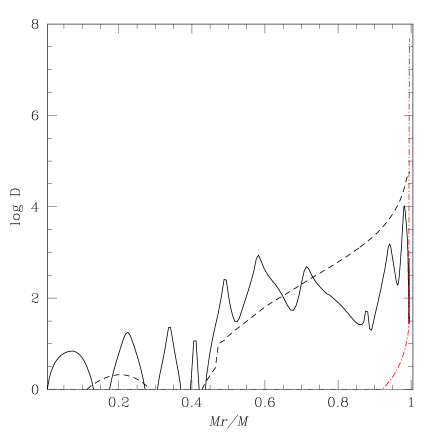
Figure 15: Total diffusion coefficient in a $1.2\,M_{\odot}$ star at 0.5 Gyr in a simple rotating model (dotted line) and in a rotating model including IGW (full line). The dashed-dotted line gives $D_{\rm waves}$.

7.4 Evolution of Chemicals

Our goal in the present paper is not to make detailed comparison of the model predictions with all the observable constraints that come from abundance anomalies in stars. This will be done in forthcoming studies. We wish however to illustrate briefly the behavior of ⁴He and ⁷Li in our $1.2\leavevmode\nobreak\ M_{\odot}$ rotating model including gravity waves. The case of ⁴He is related to possible impact on the overall evolution and lifetimes, and in addition it illustrates the interaction with atomic diffusion. On the other hand ⁷Li is a fragile element which helps to probe the status of the external stellar layers.

The ⁴He profile at the age of the Hyades is shown in Fig. 16 for both the complete model and the model without IGW. One sees there two effects. First, at this age, the model with IGW is slightly less evolved (i.e. it has a lower central ⁴He content). Second, its ⁴He surface abundance is slightly lower and the ⁴He gradient just below the convection envelope is slightly steeper. This is due to the lower amplitude of the total diffusion coefficient in the models including waves, which allows ⁴He to settle more under the effect of atomic diffusion. One sees here that $D_{\rm waves}$ has a negligible effect on the ⁴He behavior and does not compensate for the decrease in the total diffusion coefficient in the external part of the radiative zone.

The best observational constraints available to test our predictions are the Li data in open clusters. As discussed in § 1, models in which the transport of angular momentum is carried out only by meridional circulation and turbulence fail to reproduce the rise of the Li abundance on the right side of the Li dip. This is confirmed in the present model without IGW which lies in this region and has an effective temperature of $T_{\rm eff}=6220\leavevmode\nobreak\ {\rm K}$ at the age of the Hyades. As can be seen in Fig. 17, the ⁷Li surface abundance in this model (dotted line) is $\sim$ one order of magnitude smaller than the Li value in stars of $6220\pm 100\leavevmode\nobreak\ {\rm K}$ in the Hyades and which is indicated by the box. For the model including IGW (full line), the magnitude of both meridional circulation and turbulence is reduced. Consequently ⁷Li is less destroyed and our prediction accounts nicely for the data. Note that the surface lithium decrease in these stars is not dominated by atomic diffusion, but still by the (reduced, compared to the case without IGW) rotational transport of this element down to regions where it is nuclearly destroyed. Again, the effect of $D_{\rm waves}$ is negligible.

In a forthcoming paper, we will present models of Pop I stars with various initial masses and initial rotation rates and compare in details the Li predictions on the red side of the Li dip with observations in open cluster and field stars.

Figure 16: ⁴He profile at the age of the Hyades in the complete model (full line) and in the model without the IGW (dashed line) for a $1.2\,M_{\odot}$ star.

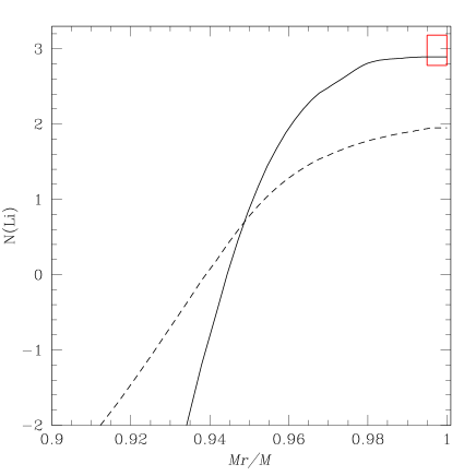
Figure 17: ⁷Li profile at the age of the Hyades in the complete model (full line) and in the model without the IGW (dashed line) for a $1.2\,M_{\odot}$ star. The box indicates the observed Li abundances in Hyades stars with an effective temperature ($\pm$ 100 K) corresponding to that of the model at 0.7 Gyr (data by Boesgaard & King 2002)

8 Discussion and Conclusions

In this paper, we examined how it is possible to include all the effects of internal gravity waves into evolutionary calculations. The main challenge is that IGW tend to produce a thin shear layer that oscillates with a very small time-scale. Talon et al. (2002) showed that this shear layer oscillation (or SLO) acts as a filter for waves, being more transparent to waves that will reduce the differential rotation between the convection and the radiation zones. We verified that this filter is linear in $\delta\Omega$ and as such, details of the SLO need not be considered for variations occurring over long time-scales.

We also presented the first evolution model that includes the hydrodynamical processes induced by rotation and internal gravity waves. We focused on a $1.2\leavevmode\nobreak\ M_{\odot}$, $Z=0.02$ star which lies on the red side of the Li dip ($T_{\rm eff}=6220\,{\rm K}$ at 0.7 Gyr). For the rotation profile, IGW lead to the appearance of a “slow” front, propagating from the core to the surface. When the outer convection zone is constantly spun down, several fronts propagate; this propagation is very rapid at the beginning because differential rotation is large, and slows down with time.

For the evolution of chemicals, Talon & Charbonnel (1998) expected IGW to reduce rotational mixing together with differential rotation. This effect is confirmed in this first fully consistent study. The surface of the Li abundance in our complete model is in perfect agreement with the data in the Hyades stars of similar effective temperature.

Let us remind to the reader that, while the formalism presented in this paper is quite general and allows to properly include IGW in complete hydrodynamical stellar models, several uncertainties remain. Firstly, a very delicate issue is that of IGW generation. The GMK model most certainly underestimates the wave flux since it considers only bulk excitation, and not overshooting or convective penetration. However, since wave generation has to be proportional to the convective luminosity, differential properties between different stellar types should vary less. We thus expect the wave flux to be larger than calculated, but by a similar amount in each stellar type. Complete studies for different stellar types should permit to calibrate this amount, that could then be used uniformly.

The second uncertainty is the exact value for the turbulent viscosity to use in the SLO ($\nu_{\rm waves}$, Eq. 17). Here, we estimated a viscosity based on the shear instability and assumed a small amount of enlargement and averaging in order for the turbulent viscosity not to be too local. However, this model has only a rather small impact on numerical results since in all cases it remains very localized below the convection zone.

The last point to bear in mind is that no latitudinal dependence is considered here; only a horizontal average is used. Let us remark that, in order to be able to take into account this dependence, observational data of latitudinal differential rotation in stars other than the Sun must be obtained.

The results on the evolution of the rotation profile and on the lithium abundance presented in this paper are very encouraging and should now to be confronted to the data for stars of various masses, metallicities and ages. This will be done in forthcoming studies.

- [1] Alexander D.R., Ferguson J.W., 1994, ApJ, 437, 879
- [2] Andersen B.N., 1994, Solar Phys. 152, 241
- [3] Andersen B.N., 1996, A&A 312, 610
- [4] Ando H., 1986, A&A 163, 97
- [5] Angulo C., Arnould M., Rayet M., et al., 1999, Nucl.Phys.A, 656, 3
- [6] Balmforth N.J., 1992, MNRAS 255, 639
- [7] Barnes G., Charbonneau P., MacGregor K.B., 1999, ApJ, 511, 762
- [8] Boesgaard A.M., King J.R., 2002, ApJ 565, 587
- [9] Bretherton F.P., 1969, Quart. J. R. Met. Soc. 95, 213
- [10] Brown T.M., Christensen-Dalsgaard J., Dziembowski W.A., Goode P., Gough D.O., Morrow C.A., 1989, ApJ 343, 526
- [11] Canuto V.M., 2002, MNRAS 337, 713
- [12] Chaboyer B., Demarque P., Guenther D.B., Pinsonneault M.H., 1995, ApJ 446, 435
- [13] Chaboyer B., Zahn J.P., 1992, A&A 253, 173
- [14] Charbonneau P., MacGregor K.B., 1993, ApJ, 417, 762
- [15] Charbonneau P., Michaud, G., 1988, ApJ, 334, 746
- [16] Charbonnel C., Talon S., 1999, A&A 351, 635 1997, A&A 324, 298
- [17] Couvidat S., Garcia R.A., Turck-Chièze S., Corbard T., Henney C.J., Jiménez-Reyes S., 2003, ApJ 597, L77
- [18] Dudis J.J., 1974, J. Fluid Mech. 64, 65 Wheeler S.J., Gough D.O., 1995, Nature 376, 669
- [19] Forestini M., 1991, PhD thesis, Université Libre de Bruxelles, Belgium
- [20] Fritts D.C., Vadas S.L., Andreassen Ø., 1998, A&A 333, 343
- [21] Gaigé Y., 1993, A&A 269, 267
- [22] García López R.J., Spruit H.C., 1991, ApJ 377, 268
- [23] Goldreich P., Keeley D.A., 1977, ApJ 212, 243
- [24] Goldreich P., Kumar P., 1990, ApJ 363, 694
- [25] Goldreich P., Murray N., Kumar, P., 1994, ApJ 424, 466
- [26] Goldreich P., Nicholson P.D., 1989, ApJ 342, 1079
- [27] Gough D. O., McIntyre M.E., 1998, Nature 394, 755
- [28] Hurlburt N.E., Toomre J., Massaguer J.M., 1986, ApJ 311, 563
- [29] Hurlburt N.E., Toomre J., Massaguer J.M., Zahn J.-P., 1994, ApJ 421, 245
- [30] Iglesias C.A., Rogers F.J., 1996, ApJ 464, 943
- [31] Kawaler S.D., 1988, ApJ 333, 236
- [32] Kim Eun-jin, MacGregor K.B., 2001, ApJ 556, L117
- [33] Kim Eun-jin, MacGregor K.B., 2003, ApJ 588, 645
- [34] Kiraga M., Jahn K., Stepien K., Zahn J.-P., 2003, Acta Astronomica, 53, 321
- [35] Kiraga M., Różyczka M., Stepien K., Jahn K., Muthsam H., 2000, Acta Astronomica, 50, 93
- [36] Kosovichev A., et al., 1997, Sol. Phys. 170, 43
- [37] Kumar P., Quataert E.J., 1997, ApJ 475, L143
- [38] Kumar P., Talon S., Zahn J.-P., 1999, ApJ 520, 859 (KTZ)
- [39] Lignières F., Califano F., Mangeney A., 1999, A&A 314, 465
- [40] Matias J., Zahn J.-P., 1998, in “Sounding solar and stellar interiors”, IAU Symposium 181, poster volume, Eds. Provost J. & Schmider F.X.
- [41] Maeder A., 1995, A&A 299, 84
- [42] Maeder A., 2003, A&A 399, 263
- [43] Maeder A., Meynet G., 2000, ARAA 38, 143
- [44] Maeder A., Meynet G., 2003, A&A 411, 552
- [45] Maeder A., Meynet G., 2004, A&A 422, 225
- [46] Maeder A., Zahn J.P., 1998, A&A 334, 1000
- [47] Meynet G., Maeder A., 2005, A&A 429, 581
- [48] Montalbán J., 1994, A&A 281, 421
- [49] Montalbán J., Schatzman E., 1996, A&A 305, 513
- [50] Montalbán J., Schatzman E., 2000, A&A 354, 943
- [51] Nordlund A., Stein R.F., Brandenburg A., 1996, Bull. Astron. Soc. of India 24, 261
- [52] Palacios A., Charbonnel C., Talon S., Siess L., 2005, in preparation
- [53] Palacios A., Talon S., Charbonnel C., Forestini M., 2003, A&A 399, 603
- [54] Paquette C., Pelletier C., Fontaine G., Michaud G., 1986, ApJS, 61, 177
- [55] Pasquini L., Randich S., Zoccali M., Hill V., Charbonnel C., Nordström B., 2004, A&A 424, 951
- [56] Pinsonneault M., Kawaler S.D., Sofia S., Demarque P., 1989, ApJ, 338, 424
- [57] Pols O.R., Tout C.A., Eggleton P.P., Han Z., 1995, MNRAS, 274, 964
- [58] Press W.H., 1981, ApJ 245, 286
- [59] Rogers T.M., Glatzmeier G.A., 2005, ApJ 620, 432
- [60] Ringot O., 1998, A&A 335, 89
- [61] Schatzman E., 1993, A&A 279, 431
- [62] Siess L., Dufour, E., Forestini M., 2000, A&A 358, 593
- [63] Siess L., Forestini M., Bertout C., 1996, A&A 326, 1001
- [64] Spruit H.C., 1999, A&A 349, 189
- [65] Spruit H.C., 2002, A&A 381, 923
- [66] Talon S., 2004, in “Stellar Rotation”, IAU Symposium 215, Eds. André Maeder & Philippe Eenens
- [67] Talon S., Charbonnel C., 1998, A&A 335, 959
- [68] Talon S., Charbonnel C., 2003, A&A 405, 1025
- [69] Talon S., Charbonnel C., 2004, A&A 418, 1051
- [70] Talon S., Kumar P., Zahn J.-P., 2002, ApJL 574, 175 (TKZ)
- [71] Talon S., Zahn J.-P., 1997, A&A 317, 749
- [72] Talon S., Zahn J.P., Maeder A., Meynet G., 1997, A&A 322, 209
- [73] Townsend A.A., 1958, J. Fluid Mech. 4, 361
- [74] Townsend A.A., 1965, J. Fluid Mech. 22, 241
- [75] Turcotte S., Richer J., Michaud G., Iglesias C.A., Rogers F.J., 1998, ApJ 504, 539
- [76] Young P.A., Knierman K.A., Rigby J.R., Arnett D., 2003, ApJ 595, 1114
- [77] Zahn J.P., 1992, A&A 265, 115
- [78] Zahn J.-P., Talon S., Matias J., 1997, A&A 322, 320