New model of angular momentum transfer from the rotating central body of a two-body system into the orbital motion of this system (with application to the earth-moon system)

Abstract

In a previous paper we treated within the framework of our Projective Unified Field Theory (Schmutzer 2004, Schmutzer 2005a) the 2-body system (e.g. earth-moon system) with a rotating central body in a rather abstract manner. Here a concrete model of the transfer of angular momentum from the rotating central body to the orbital motion of the whole 2-body system is presented, where particularly the transfer is caused by the inhomogeneous gravitational force of the moon acting on the oceanic waters of the earth, being modeled by a spherical shell around the solid earth. The theory is numerically tested.
Key words: transfer of angular momentum from earth to moon, action of the gravitational force of the moon on the waters of the earth.

1 Introduction

Nowadays the concept that the tidal braking effect of the earth rotation is caused by the gravitational force of the moon acting on the viscous oceanic waters around the earth is accepted in general. With respect to the details of this braking mechanism several models were proposed and theoretically investigated in detail, including numerical computer calculation. We refrain from reviewing the historically first ideas and the afterwards following publications on this subject, but we rather cite some previous papers, where the interested reader can find further information: Brosche 1975, 1979, 1989 as well as Brosche and Schuh 1998.

Our considerations start with a strongly simplified model of the earth consisting of a rigid sphere surrounded by a homogeneous viscous fluid shell (oceanic waters) of uniform thickness, being under the influence of the rotation and the gravitational field of the rigid earth as well as of the gravitational field of the orbiting moon. It may be a good help to the reader to have a look on the figures of forming of the tidal bulge mechanism without and with phase lag in both the monographs: Lambeck 1980, Sabadini and Vermeersen 2004. For this publication the physical situation of the earth-moon system with phase lag is sketched in Fig. 2.

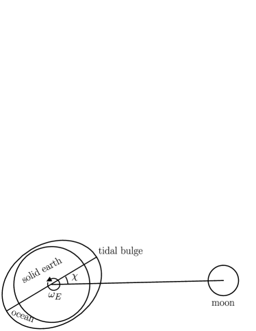
Figure 1: Deformed fluid shell (deformation caused by the gravitational field of the moon) including the rotation of the earth, which causes the phase lag by the dragging effect within the viscous fluid.

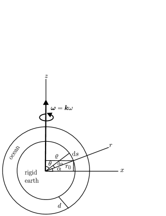
Figure 2: Rigid earth, ocean as viscous fluid shell and line element $\;\mathrm{d}s$ at the interface between both parts of the earth ($r_{0}$ radius of the rigid earth).

For the concrete calculations in the following sections we use Fig. 2 (axis of rotation $\rightarrow$ $z$-axis) and Fig. 3 (axis of rotation $\rightarrow$ perpendicular to the $x$-$y$-plane).

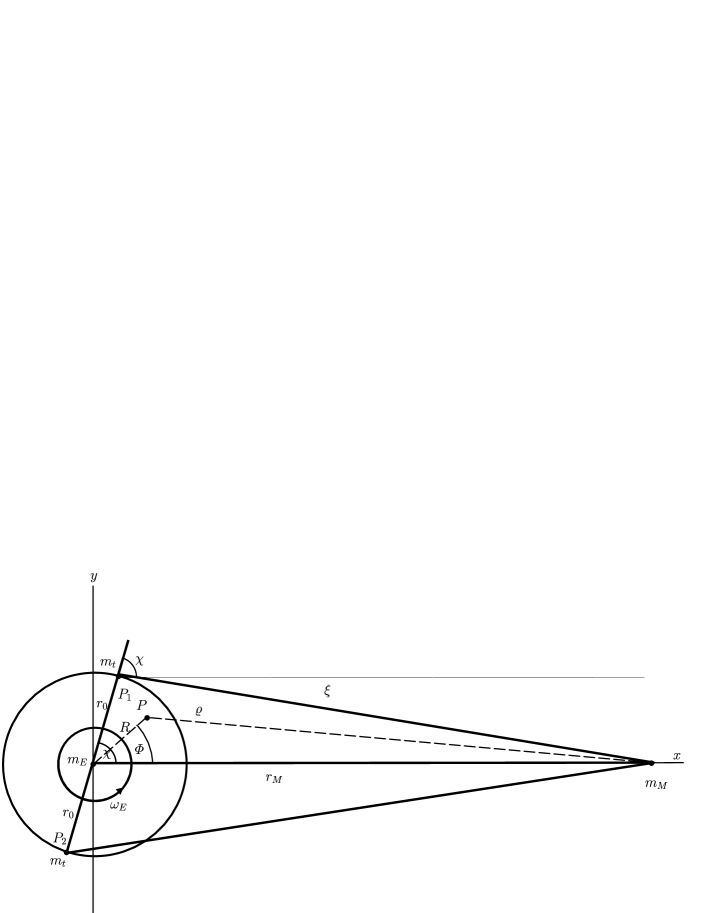
Figure 3: Equilibrium of the tidal bulge (quasi-mechanical body with mass $m_{t}$ in the point $P_{1}$) as a result of the acting gravitational force of the moon and the dragging force (negative friction force) within the fluid, caused by rotation of the earth.

2 Friction force and friction torque

Now using Fig. 2, we apply Newton’s friction force law to the infinitesimal azimuthal component of the friction force $\;\mathrm{d}F_{fric|\varPhi}$ within a viscous fluid ($\eta$ viscosity), referring to an infinitesimal areal element $\;\mathrm{d}A_{\varPhi}$ positioned at the point with the cylindrical coordinates ($\varrho=r_{0}\cos\alpha$, $\varPhi$, $z=r_{0}\sin\alpha$) at the bottom of the ocean:

$$\begin{aligned} &\mbox{a)}\quad\;\mathrm{d}F_{fric|\varPhi}=\eta\mbox{$\displaystyle\frac{{\rm d}v}{{\rm d}r}$}\,\;\mathrm{d}A_{\varPhi}=r_{0}^{2}\mbox{$\displaystyle\frac{{\rm d}v}{{\rm d}r}$}\,\cos\alpha\;\mathrm{d}\varPhi\;\mathrm{d}\alpha\quad\text{with}\\ &\mbox{b)}\quad\;\mathrm{d}A_{\varPhi}=\varrho\;\mathrm{d}\varPhi\;\mathrm{d}s\,,\quad\mbox{c)}\quad\;\mathrm{d}s=r_{0}\;\mathrm{d}\alpha\,,\quad\mbox{d)}\quad v=\omega\varrho=r_{0}\omega\cos\alpha\end{aligned}$$ (1)

($r_{0}$ radius of the earth, $v$ radial-dependent azimuthal velocity, $\omega$ rotational angular velocity).

In vectorial writing the corresponding infinitesimal friction force reads:

$$\;\mathrm{d}\boldsymbol{F}_{fric|\varPhi}=\boldsymbol{e}_{\varPhi}\;\mathrm{d}F_{fric|\varPhi}\,.$$ (2)

Because of the rotation-symmetry assumed we find by integration over the azimuthal angle $\varPhi$ from $0$ to $2\pi$ the intermediate results

$$\mbox{a)}\quad\;\mathrm{d}A=\int\limits_{0}^{2\pi}\;\mathrm{d}A_{\varPhi}=2\pi r_{0}^{2}\cos\alpha\;\mathrm{d}\alpha\,,\quad\mbox{b)}\quad\;\mathrm{d}F_{fric}=\eta\mbox{$\displaystyle\frac{{\rm d}v}{{\rm d}r}$}\,\;\mathrm{d}A\,.$$ (3)

For simplification of the problem we suppose a linear radial velocity profile ($d$ depth of the ocean):

$$\mbox{a)}\quad v(r,\alpha)=v(r_{0},\alpha)\Bigl{[}1-\frac{1-s_{oc}}{d}\,(r-r_{0})\Bigr{]}\,,\quad\text{i.e.}\quad\mbox{b)}\quad\mbox{$\displaystyle\frac{{\rm d}v(r,\alpha)}{{\rm d}r}$}=-\frac{1-s_{oc}}{d}\,v(r_{0},\alpha)\,,$$ (4)

where

$$v_{d}(\alpha)=s_{oc}v(r_{0},\alpha)$$ (5)

is the velocity at the surface of the ocean. We name the constant $s_{oc}<1$ “oceanic flow slope parameter”.

Eliminating the velocity gradient in (3b), we find

$$\;\mathrm{d}F_{fric}=-\frac{\eta(1-s_{oc})v(r_{0},\alpha)}{d}\,\;\mathrm{d}A$$ (6)

and further with the help of (3a) and (1d)

$$\;\mathrm{d}F_{fric}=-\frac{2\pi r_{0}^{3}\omega\eta(1-s_{oc})\cos^{2}\alpha}{d}\,\;\mathrm{d}\alpha\,.$$ (7)

Integration over $\alpha$ from $-\dfrac{\pi}{2}$ to $\dfrac{\pi}{2}$ yields

$$F_{fric}=-\frac{\pi^{2}r^{3}_{0}\omega\eta(1-s_{oc})}{d}\,.$$ (8)

Adapting this uniform oceanic shell modeling to the earth, where about 70.8 % of the surface are oceanic waters, it is convenient to introduce a rough “surface correction factor” $f_{oc}$. Then formula (8) reads

$$F_{fric}=-\frac{\pi^{2}r^{3}_{0}\omega\eta(1-s_{oc})f_{oc}}{d}\,.$$ (9)

As an example one is tempted to choose $f_{oc}\approx 0.6$.

Now we define in the usual way the infinitesimal vectorial friction torque

$$\;\mathrm{d}\boldsymbol{M}_{fric|\varPhi}=\boldsymbol{e}_{r}r_{0}\times\;\mathrm{d}\boldsymbol{F}_{fric|\varPhi}=-\boldsymbol{e}_{\theta}r_{0}\;\mathrm{d}F_{fric|\varPhi}$$ (10)

corresponding to the infinitesimal friction force (2).

In analogy to the above calculations we receive by integration

$$\;\mathrm{d}\boldsymbol{M}_{fric}=\int\limits_{\varPhi=0}^{2\pi}\;\mathrm{d}\boldsymbol{M}_{fric|\varPhi}\;\mathrm{d}\varPhi=-\boldsymbol{k}\frac{2\pi r_{0}^{4}\omega\eta(1-s_{oc})\cos^{3}\alpha\;\mathrm{d}\alpha}{d}$$ (11)

and by further integration

$$\boldsymbol{M}_{fric}=-\boldsymbol{k}\frac{2\pi r_{0}^{4}\omega\eta(1-s_{oc})f_{oc}}{d}\!\int\limits_{\alpha=-\frac{\pi}{2}}^{\frac{\pi}{2}}\cos^{3}\alpha\;\mathrm{d}\alpha$$ (12)

or explicitly

$$\mbox{a)}\quad\boldsymbol{M}_{fric}=\boldsymbol{k}M_{fric}\quad\text{with}\quad\mbox{b)}\quad M_{fric}=-\frac{8\pi r_{0}^{4}\omega\eta(1-s_{oc})f_{oc}}{3d}\,.$$ (13)

Let us now remember some results from our previous paper (Schmutzer 2005a): We used the following definition of the rotational angular momentum of the earth rotating about the $z$-axis:

$$\boldsymbol{L}=\boldsymbol{k}L_{rot}=\boldsymbol{k}\theta_{E}\omega_{E}$$ (14)

($\theta_{E}$ moment of inertia, $\omega_{E}$ rotational angular velocity, $\boldsymbol{k}$ unit vector in $z$-direction). Hence by temporal differentiation follows (dot means total time derivative)

$$\mbox{a)}\quad\mbox{$\displaystyle\frac{{\rm d}\boldsymbol{L}}{{\rm d}t}$}=\boldsymbol{k}\bigl{(}\dot{\theta}_{E}\omega_{E}+\theta_{E}\dot{\omega}_{E}\bigr{)}\quad\text{with}\quad\mbox{b)}\quad\dot{\theta}_{E}={}\stackrel{{\scriptstyle\circ}}{{\theta}}{\!\!}_{E}+\theta_{E}\varSigma\,.$$ (15)

From this last equation we remember that the total time derivative of the moment of inertia consists of two parts: the partial derivative (denoted by circle) and the temporal cosmological influence (determined by the “logarithmic scalaric world function” $\varSigma$).

According to the balance equation of the angular momentum

$$\mbox{$\displaystyle\frac{{\rm d}\boldsymbol{L}}{{\rm d}t}$}=\boldsymbol{M}_{fric}$$ (16)

the temporal change of $\boldsymbol{L}$ is caused by the friction torque (13a). Inserting the expression (15a) and (13a) into (16) yields the following temporal change of the angular velocity (for $\omega\to\omega_{E}$):

$$\dot{\omega}_{E}=-\frac{8\pi r_{0}^{4}\omega_{E}\eta(1-s_{oc})f_{oc}}{3\theta_{E}d}-\frac{(\stackrel{{\scriptstyle\circ}}{{\theta}}{\!\!}_{E}+\theta_{E}\varSigma)\omega_{E}}{\theta_{E}}\quad\text{or}$$ (17a)

$$\frac{\eta(1-s_{oc})f_{oc}}{d}=-\frac{3\bigl{[}\theta_{E}\dot{\omega}_{E}+(\stackrel{{\scriptstyle\circ}}{{\theta}}{\!\!}_{E}+\theta_{E}\varSigma)\omega_{E}\bigr{]}}{8\pi r_{0}^{4}\omega_{E}}\,.$$ (17b)

3 Deformation of the earth by the inhomogeneous gravitational field of the moon

Basis of our following considerations is Fig. LABEL:pic3. For treating the above physical problem further we first calculate the rotation-symmetric gravitational field of the moon (taken as point-like) about the $x$-axis ($R=\sqrt{x^{2}+y^{2}}$) under the approximate suppositions:

$$\mbox{a)}\quad\frac{r}{r_{M}}\ll 1\,,\quad\mbox{b)}\quad\frac{m_{M}r_{0}^{2}}{m_{E}r_{M}^{2}}\ll 1\,,\quad\mbox{c)}\quad\frac{m_{M}r_{0}^{3}}{m_{E}r_{M}^{3}}\ll 1$$ (18)

($m_{E}$ mass of the earth, $m_{M}$ mass of the moon, $r_{M}$ distance between the centers of earth and moon).

First we remember that the gravitational force of the moon acting on the center of the earth is compensated by the centrifugal force in this same point, caused by the orbital motion of the earth about the common center of mass of the 2-body problem.

Now we begin our considerations on the gravitational potential $\phi_{M}$ of the moon at an arbitrary point $P$ inside the earth ($r\leqq r_{0}$). Using the notation of Fig. LABEL:pic3, then the well-known Newtonian potential reads

$$\phi_{M}(\varrho)=-\frac{\gamma_{\mathrm{N}}m_{M}}{\varrho}\,.$$ (19)

Hence for the center of the earth results

$$\phi_{M}(r_{M})=-\frac{\gamma_{\mathrm{N}}m_{M}}{r_{M}}\,.$$ (20)

The difference of both the potentials is equal to

$$\varphi_{M}(\varrho)=\phi_{M}(\varrho)-\phi_{M}(r_{M})=-\gamma_{\mathrm{N}}m_{M}\Bigl{(}\frac{1}{\varrho}-\frac{1}{r_{M}}\Bigr{)}\,.$$ (21)

According to the cosine law we learn from Fig. LABEL:pic3:

$$\varrho=r_{M}\Bigl{[}1+\Bigl{(}\frac{R}{r_{M}}\Bigr{)}^{2}-\frac{2R}{r_{M}}\,\cos\varPhi\Bigr{]}^{1/2}\,.$$ (22)

With the help of (18a) we approximately find

$$\varrho=r_{M}\Bigl{[}1-\frac{R}{r_{M}}\,\cos\varPhi+\frac{1}{2}\,\Bigl{(}\frac{R}{r_{M}}\Bigr{)}^{2}\Bigl{(}1-\cos^{2}\varPhi\Bigr{)}\Bigr{]}$$ (23)

and further

$$\varphi_{M}(\varrho)=-\frac{\gamma_{\mathrm{N}}m_{M}}{r_{M}}\,\Bigl{[}\frac{R}{r_{M}}\,\cos\varPhi-\frac{1}{2}\Bigl{(}\frac{R}{r_{M}}\Bigr{)}^{2}(1-3\cos^{2}\varPhi)\Bigr{]}\,.$$ (24)

Rearranging this equation gives

$$\mbox{a)}\quad\varphi_{M}(x,y)=\frac{\gamma_{\mathrm{N}}m_{M}}{2r_{M}^{3}}\,(y^{2}-2x^{2}-2xr_{M})\quad\text{with}\quad\mbox{b)}\quad R^{2}=x^{2}+y^{2}\,.$$ (25)

With respect to the earth, for simplicity we refer to a homogeneous mass sphere. From usual textbooks we take the expression for the gravitational potential in the interior of such a homogeneous spherical body (in this notation e.g. Schmutzer 2005b):

$$\phi_{Ei}(r)=\frac{\gamma_{\mathrm{N}}m_{E}}{2r_{0}^{3}}\,(r^{2}-3r_{0}^{3})$$ (interior potential), (26a)

$$\phi_{Ee}(r)=-\frac{\gamma_{\mathrm{N}}m_{E}}{r}$$ (exterior potential). (26b)

From (25a) and (26a) we receive the superposition potential of the earth and the moon in the interior of the earth:

$$\phi_{i}(x,y)=\phi_{Ei}(x,y)+\varphi_{M}(x,y)=\frac{\gamma_{\mathrm{N}}m_{E}}{2r_{0}}\,\Bigl{[}\Bigl{(}1-\frac{2m_{M}r_{0}^{3}}{m_{E}r_{M}^{3}}\Bigr{)}\frac{(x-x_{0})^{2}}{r_{0}^{2}}+\Bigl{(}1+\frac{m_{M}r_{0}^{3}}{m_{E}r_{M}^{3}}\Bigr{)}\frac{y^{2}}{r_{0}^{2}}\Bigr{]}-\phi_{0}\,,$$ (27)

where the abbreviations

$$\mbox{a)}\quad\phi_{0}=\frac{\gamma_{\mathrm{N}}m_{M}^{2}r_{0}^{3}}{2m_{E}r_{M}^{4}\Bigl{(}1-\dfrac{2m_{M}r_{0}^{3}}{m_{E}r_{M}^{3}}\Bigr{)}}+\frac{3\gamma_{\mathrm{N}}m_{E}}{2r_{0}}\,,\quad\mbox{b)}\quad x_{0}=\frac{m_{M}r_{0}^{3}}{m_{E}r^{2}_{M}\Bigl{(}1-\dfrac{2m_{M}r_{0}^{3}}{m_{E}r_{M}^{3}}\Bigr{)}}$$ (28)

were used.

Let us here mention that the treatment of this subject in the corresponding literature usually starts from the integral representation of the potential. Our superposition method applied above lead us to the resulting ellipsoid formula by setting $\phi_{i}(x,y)=\mathrm{const}$ in (27). This approach shows that under the influence of the moon, beyond the deformation of the sphere to an ellipsoid, our calculation exhibits a translation of the resulting ellipsoid by the amount $x_{0}$ in the $x$-direction.

Using the semi-axes $\hat{a}$ and $\hat{b}$, taken from the above abbreviations,

$$\mbox{a)}\quad\hat{a}^{2}=\frac{r_{0}^{2}}{1-\dfrac{2m_{M}r_{0}^{3}}{m_{E}r_{M}^{3}}}\,,\quad\mbox{b)}\quad\hat{b}^{2}=\frac{r_{0}^{2}}{1+\dfrac{m_{M}r_{0}^{3}}{m_{E}r_{M}^{3}}}\,,$$ (29)

the equation (27) reads

$$\phi_{i}(x,y)=\frac{\gamma_{\mathrm{N}}m_{E}}{2r_{0}}\Bigl{[}\frac{(x-x_{0})^{2}}{\hat{a}^{2}}+\frac{y^{2}}{{\hat{b}}^{2}}-1\Bigr{]}+\frac{\gamma_{\mathrm{N}}m_{E}}{2r_{0}}-\phi_{0}\,.$$ (30)

Fitting this potential to the surface equation of the physical ellipsoid

$$\frac{(x-x_{0})^{2}}{\hat{a}^{2}}+\frac{y^{2}}{{\hat{b}}^{2}}=1$$ (31)

of the slightly deformed earth by the inhomogeneous gravitational field of the moon leads to the expression

$$\phi_{i}(x,y)_{\mathit{ellipsoid}}=\frac{\gamma_{\mathrm{N}}m_{E}}{2r_{0}}-\phi_{0}=-\frac{\gamma_{\mathrm{N}}m_{E}}{r_{0}}-\frac{\gamma_{\mathrm{N}}m_{M}^{2}r_{0}^{3}}{2m_{E}r^{4}_{M}\Bigl{(}1-\dfrac{2m_{M}r_{0}^{3}}{m_{E}r_{M}^{3}}\Bigr{)}}\,.$$ (32)

Further simplification of the above formula (31) is reached by applying the approximate suppositions derived from (18):

$$\mbox{a)}\quad x_{0}=\frac{m_{M}r_{0}^{3}}{m_{E}r_{M}^{2}}\,,\quad\mbox{b)}\quad\phi_{0}=\frac{3\gamma_{\mathrm{N}}m_{E}}{2r_{0}}\,,\quad\mbox{c)}\quad\hat{a}=r_{0}\Bigl{(}1+\frac{m_{M}r_{0}^{3}}{m_{E}r_{M}^{3}}\Bigr{)}\,,\quad\mbox{d)}\quad\hat{b}=r_{0}\Bigl{(}1-\frac{m_{M}r_{0}^{3}}{2m_{M}r_{M}^{3}}\Bigr{)}\,.$$ (33)

Conservation of the mass of the earth

$$m_{E}=\frac{4\pi}{3}\,\mu_{0}r_{0}^{3}$$ (34)

($\mu_{0}$ constant mass density) during the deformation leads to the relation

$$r_{0}^{3}=\hat{a}{\hat{b}}^{2}\,.$$ (35)

One should remember that for simplicity our above calculations were based on a homogeneous mass model of the earth. For our further calculations we are only interested in the physical situation at the surface of the sphere, not explicitly referring to its interior. Therefore our further treatment is consistent.

4 Rotation of the earth, dragging force on the tidal bulges and calculation of the tidal phase lag angle (tidal dragging angle)

4.1 Forces on the moon-nearest bulge

Nowadays there is no doubt among the experts that the phenomenon of the oceanic tides is primarily caused by the moon. The observed tidal water bulges in the zenith (direction to the moon) and symmetric to it in the nadir (opposite direction) are modeled by the two water bulges resulting from the symmetric deformation of the sphere to the ellipsoidal form calculated above. Since the rotational angular velocity of the earth is much bigger than the revolution angular velocity of the moon, the earth performs a relatively quick rotation with respect to the tidal bulges, i.e. with respect to the moon (motion under the quasi-fixed bulges). Hence follows that an observer in the frame of reference of the surface of the earth realizes the phenomenon of tides.

Here we investigate the dragging effect of the viscous waters, caused in the waters by the rotation of the rigid earth. This effect leads to a shift of the bulges by a certain phase lag angle $\chi$. The equilibrium position of the bulges is the result of two on the bulges acting torques, caused by the gravitational force of the moon and the dragging force in the viscous oceanic waters, as above already mentioned.

Our task is now to determine this equilibrium position of the moon-nearest bulge which abstractively will be considered as a mechanical quasi-body, where the forces act on the center of mass of this quasi-body ($m_{t}$ tidally caused mass of the quasi-body). The following investigations are based on Fig. LABEL:pic3, where for simplicity the ellipsoid is approximated by a sphere and the point of consideration is shifted from the interior to the surface of the earth ($P\to P_{1}$).

Let us further mention that the gravitational force of the sun, which is distinctly smaller than the gravitational force of the moon, will be neglected for simplification of the physical problem, i.e. we concentrate our investigation on the primarily essential points of the equilibrium mechanism.

In order to calculate the resulting torque acting on the center of mass of the moon-nearest bulge, we first list the various forces being present:

$$\boldsymbol{F}_{E}=m_{t}\boldsymbol{G}_{E}=m_{t}\boldsymbol{e}_{R}G_{E|R}$$ (36)

(radial gravitational force of the earth),

$$\boldsymbol{F}_{M}=m_{t}\boldsymbol{G}_{M}$$ (37)

(radial gravitational force of the moon),

$$\boldsymbol{F}_{c}=m_{t}\boldsymbol{G}_{c}=m_{t}\boldsymbol{e}_{R}r_{0}\omega_{E}^{2}$$ (38)

(radial centrifugal force by rotation of the earth),

$$\boldsymbol{F}_{fric}=\boldsymbol{e}_{\varPhi}F_{fric}$$ (39)

(azimuthal friction force determined by (9)),

$$\boldsymbol{F}_{p}=\boldsymbol{e}_{R}F_{p|R}$$ (40)

(radial pressure force on the bulge as back-reaction of the earth).

One should realize that the quantities $\boldsymbol{G}_{E}$, $\boldsymbol{G}_{M}$ and $\boldsymbol{G}_{c}$ are acceleration quantities.

Using the radial and azimuthal vectorial decomposition of (37), we obtain

$$\mbox{a)}\quad\boldsymbol{F}_{M}=\boldsymbol{e}_{R}F_{M|R}+\boldsymbol{e}_{\varPhi}F_{M|\varPhi}\quad\text{with}\quad\mbox{b)}\quad F_{M|R}=m_{t}G_{M|R}\,,\quad\mbox{c)}\quad F_{M|\varPhi}=m_{t}G_{M|\varPhi}\,.$$ (41)

Hence follows the radial component of the total force as the sum of all radial components:

$$F_{R}=m_{t}\bigl{(}G_{E|R}+G_{M|R}+r_{0}\omega_{E}^{2}\bigr{)}+F_{p|R}\,.$$ (42)

4.2 Stationary equilibrium

Demanding stationarity we arrive at the equation

$$F_{R}=0\,.$$ (43)

With respect to the azimuthal component of the force we meet the following physical situation: Due to the viscosity of the fluid the quasi-body (modeled bulge) is dragged into the direction of the rotational orbital velocity by the dragging force

$$F_{drag}=-F_{fric}\qquad\text{($F_{drag}>0$, $F_{fric}<0$).}$$ (44)

In the case of stationarity the dragging force is compensated by the (oppositely directed) gravitational force (pulling force) of the moon.

These previous considerations lead us to the equilibrium equation

$$F_{\varPhi}=F_{M|\varPhi}+F_{drag}=m_{t}G_{M|\varPhi}+F_{drag}=0$$ (45)

being by means of (44) equivalent to the condition

$$F_{fric}=m_{t}G_{M|\varPhi}\,.$$ (46)

According to the definition of the torque by the azimuthal forces

$$M_{\varPhi}=F_{\varPhi}r_{0}\,,$$ (47)

for the equilibrium results

$$M_{\varPhi}=0\,,$$ (48)

being equivalent to (45).

4.3 Calculation of the azimuthal gravitational force component and of the gravitational torque, both caused by the moon

After these decomposition procedures we are now able to calculate on the basis of Fig. LABEL:pic3 the azimuthal component of the gravitational force of the moon acting on the tidal bulge being at the oceanic surface of the earth ($R\to r_{0}$, $\varPhi\to\chi$). In this specialization formula (23) reads

$$\xi=r_{M}\Bigl{[}1-\frac{r_{0}}{r_{M}}\,\cos\chi+\frac{1}{2}\,\Bigl{(}\frac{r_{0}}{r_{M}}\Bigr{)}^{2}(1-\cos^{2}\chi)\Bigr{]}\,.$$ (49)

By differentiation follows

$$\,\mbox{$\displaystyle\dfrac{{\partial}\xi}{{\partial}\chi}$}\,=r_{0}\sin\chi\Bigl{(}1+\frac{r_{0}}{r_{M}}\,\cos\chi\Bigr{)}\,.$$ (50)

We further receive with the help of (49) from (19)

$$\phi_{M}(\xi)=-\frac{\gamma_{\mathrm{N}}m_{M}}{r_{M}}\,\Bigl{[}1+\frac{r_{0}}{r_{M}}\,\cos\chi-\frac{1}{2}\,\Bigl{(}\frac{r_{0}}{r_{M}}\Bigr{)}^{2}(1-3\cos^{2}\chi)\Bigr{]}$$ (51)

and hence by differentiation

$$\,\mbox{$\displaystyle\dfrac{{\partial}\phi_{M}(\xi)}{{\partial}\xi}$}\,=\frac{\gamma_{\mathrm{N}}m_{M}}{r_{M}^{2}}\,\Bigl{[}1+\frac{2r_{0}}{r_{M}}\,\cos\chi-\Bigl{(}\frac{r_{0}}{r_{M}}\Bigr{)}^{2}(1-4\cos^{2}\chi)\Bigr{]}\,.$$ (52)

By means of (52) and (50) follows

$$\,\mbox{$\displaystyle\dfrac{{\partial}\phi_{M}}{{\partial}\chi}$}\,=\,\mbox{$\displaystyle\dfrac{{\partial}\phi_{M}(\xi)}{{\partial}\xi}$}\,\,\mbox{$\displaystyle\dfrac{{\partial}\xi}{{\partial}\chi}$}\,=\frac{\gamma_{\mathrm{N}}m_{M}r_{0}\sin\chi}{r_{M}^{2}}\,\Bigl{[}1+\frac{3r_{0}}{r_{M}}\,\cos\chi-\Bigl{(}\frac{r_{0}}{r_{M}}\Bigr{)}^{2}(1-6\cos^{2}\chi)\Bigr{]}\,.$$ (53)

This result leads to the azimuthal gravitational force of the moon, acting on the moon-nearest tidal bulge at the azimuthal angle $\chi$ (first order approximation in $r_{0}$):

$$F_{M\chi}=m_{t}G_{M\chi}=-m_{t}\,\mbox{$\displaystyle\dfrac{{\partial}\phi_{M}}{{\partial}(r_{0}\chi)}$}\,=-\frac{\gamma_{\mathrm{N}}m_{M}m_{t}\sin\chi}{r_{M}^{2}}\,\Bigl{(}1+\frac{3r_{0}}{r_{M}}\,\cos\chi\Bigr{)}\,.$$ (54)

Hence by the angle transformation $\chi\to\chi+\pi$ we arrive at the corresponding force on the diagonally situated second tidal bulge:

$$F_{M(\chi+\pi)}=\frac{\gamma_{\mathrm{N}}m_{M}m_{t}\sin\chi}{r_{M}^{2}}\,\Bigl{(}1-\frac{3r_{0}}{r_{M}}\,\cos\chi\Bigr{)}\,.$$ (55)

From (54) and (55) we find for the azimuthal gravitational force of the moon, acting on both tidal bulges:

$$F_{M|az}=F_{M\chi}+F_{M(\chi+\pi)}=-\frac{3\gamma_{\mathrm{N}}m_{M}m_{t}r_{0}}{r_{M}^{3}}\,\sin(2\chi)\,.$$ (56)

The corresponding azimuthal gravitational torque, caused by the moon, reads:

$$M_{M|az}=F_{M|az}r_{0}\,.$$ (57)

4.4 Tidal phase lag angle (dragging angle)

This quantity follows immediately from the stationary equilibrium condition (45). Inserting (56) and (8) into this condition gives the intended result ($\omega\to\omega_{E}$ angular velocity of the earth):

$$\mbox{a)}\quad\sin(2\chi)=\frac{\pi^{2}r_{0}^{2}r_{M}^{3}\omega_{E}\eta(1-s_{oc})f_{oc}}{3\gamma_{\mathrm{N}}m_{M}m_{t}d}\quad\text{or}\quad\mbox{b)}\quad\chi=\frac{1}{2}\,\arcsin\frac{\pi^{2}r_{0}^{2}r_{M}^{3}\omega_{E}\eta(1-s_{oc})f_{oc}}{3\gamma_{\mathrm{N}}m_{M}m_{t}d}$$ (58)

($\chi$ tidal phase lag angle or dragging angle).

For practical reasons we approximate (58a) for the case $|\chi|\ll\dfrac{1}{2}$:

$$\chi=\frac{\pi^{2}r_{0}^{2}r_{M}^{3}\omega_{E}\eta(1-s_{oc})f_{oc}}{6\gamma_{\mathrm{N}}m_{M}m_{t}d}\,.$$ (59)

Further it is useful to introduce the meaningful quantity

$$S_{tidal}=\frac{\eta(1-s_{oc})f_{oc}}{dm_{t}\chi}$$ (60)

which we name “tidal coefficient”.

By means of (59) we receive the following different form of it:

$$S_{tidal}=\frac{6\gamma_{\mathrm{N}}m_{M}}{\pi^{2}r_{0}^{2}r_{M}^{3}\omega_{E}}\,,$$ (61)

In this context we remember the relation (17b). Neglecting the rebound effect, cosmological effect, etc., from this relation mentioned we find

$$\frac{\eta(1-s_{oc})f_{oc}}{d}=-\frac{3\theta_{E}\dot{\omega}_{E|tidal}}{8\pi r_{0}^{4}\omega_{E}}\,.$$ (62)

Eliminating in (60) with the help of this formula, we obtain the following alternative relation for the tidal coefficient:

$$S_{tidal}=-\frac{3\theta_{E}\dot{\omega}_{E|tidal}}{8\pi r_{0}^{4}\omega_{E}m_{t}\chi}\,.$$ (63)

5 Numerical evaluation

5.1 Empirical values

First from the corresponding literature we list some empirical data on the earth-moon system etc., being useful for the following numerical calculations (Gauss system of units):

$$\gamma_{\mathrm{N}}=6.673\cdot 10^{-8}\,\mathrm{g^{-1}cm^{3}s^{-2}}$$ (64)

(Newtonian gravitational constant),

$$r_{0}=6.378\cdot 10^{8}\,\mathrm{cm}$$ (65)

(radius of the earth),

$$r_{M}=3.844\cdot 10^{10}\,\mathrm{cm}$$ (66)

(distance earth/moon),

$$m_{E}=5.976\cdot 10^{27}\,\mathrm{g}$$ (67)

(mass of the earth),

$$m_{M}=7.348\cdot 10^{25}\,\mathrm{g}$$ (68)

(mass of the moon).

$$\omega_{E}=7.292\cdot 10^{-5}\,\mathrm{s^{-1}}$$ (69)

(angular velocity of the earth),

$$\dot{\omega}_{E|tidal}=-6.15\cdot 10^{-22}\,\mathrm{s^{-2}}$$ (70)

(tidal braking angular acceleration of the earth),

$$\mu_{oc}\approx 1.025\,\mathrm{g\,cm^{-3}}\qquad\text{[IERS Conventions 2003]}$$ (71)

(average mass density of the oceanic waters),

$$\theta_{E}=C_{E}=8.039\cdot 10^{44}\,\mathrm{g\,cm^{2}}$$ (72)

(polar moment of inertia of the earth).

Let us here add two remarks:

1. The values listed above partly serve as data for approximate information.

2. The following numerical calculations are performed for rough testing our theory with respect to the order of magnitude.

5.2 Detailed numerical results by using values of the above list

From (61) we determine the tidal coefficient:

$$S_{tidal}=1.77\cdot 10^{-27}\,\mathrm{cm^{-2}s^{-1}}\,,$$ (73)

whereas from (63) we find

$$m_{t}\chi S_{tidal}=4.91\cdot 10^{-9}\,\mathrm{g\,cm^{-2}s^{-1}}\,.$$ (74)

Using the value (73), we arrive at

$$m_{t}\chi=2.77\cdot 10^{18}\,\mathrm{g}\,.$$ (75)

As empirically observed, the tide is coming in approximately 25 minutes after the culmination of the moon. This fact corresponds to a phase lag angle of

$$\mbox{a)}\quad\chi=6.25^{\circ}=0.11\,\mathrm{rad}\,,\quad\text{i.e.}\quad\mbox{b)}\quad\sin\chi=0.112\,.$$ (76)

Inserting the first value into (75), we find for the mass of the tidal bulge the numerical result

$$m_{t}=2.54\cdot 10^{19}\,\mathrm{g}\,.$$ (77)

Since we here are mainly interested in orders of magnitudes of some physical quantities, we refrain from refinements of our rough oceanic shell model. For simplicity we therefore choose for the thickness of the shell the estimated average value

$$d=3.8\cdot 10^{5}\,\mathrm{cm}=3.8\,\mathrm{km}$$ (78)

to be found in literature. Further for our refinement parameters we take the simple values $s_{oc}=0$, $f_{oc}=1$.

Then from (60) results

$$\mbox{a)}\quad S_{tidal}=\frac{\eta}{dm_{t}\chi}\quad\text{or}\quad\mbox{b)}\quad\eta=S_{tidal}dm_{t}\chi\,.$$ (79)

Using the above numerical values (73), (76a), (77) and (78), we arrive at the following approximate value of the viscosity of the oceanic waters

$$\eta=1.87\cdot 10^{-3}\,\mathrm{g\,cm^{-1}s^{-1}}=1.87\cdot 10^{-3}\,\mathrm{Poise}\quad\text{($1\,\mathrm{Poise}=1\,\mathrm{g\,cm^{-1}s^{-1}}$)}$$ (80)

which, considering our rough shell model, seems not to be too far away from empirical viscosity values of water, e.g. $\eta_{water}\approx 10^{-2}\,\mathrm{Poise}$ at $20^{\circ}\,\mathrm{C}$.

Finally we estimate the seize of the tidal bulge, up to now roughly treated as a quasi-mechanical body. We approximate such a body by a spherical cap whose volume is given by the formula ($R$ radius of the cap, $h$ height of the cap)

$$V_{cap}=\frac{\pi h}{6}\,(3R^{2}+h^{2})\,.$$ (81)

Rearranging this equation leads us to the following formula for the radius of the cap:

$$R=\sqrt{\dfrac{2m_{t}}{\pi\mu_{oc}h}-\dfrac{1}{3}\,h^{2}}\,.$$ (82)

Taking from literature the approximate empirical value of the height of the tide cap $h=53\,\mathrm{cm}$, by means of (71) and (77) we receive for the radius of the cap the numerical value

$$R=5.46\cdot 10^{8}\,\mathrm{cm}=5460\,\mathrm{km}\,.$$ (83)

Thankfully I appreciate interesting discussions with Prof. P. Brosche (Observatory Hoher List) and the technical help of Prof. A. Gorbatsievich (University of Minsk).

References

• Brosche, P.: 1975, Naturwissenschaften 62, (p.1-9); 1979, Astron. Nachr. 300, (p.195-196); 1989, Physik in unserer Zeit (Geophysik), 20.Jahrgang, Nr. 3, (p.70-78)

• Brosche, P. , Schuh, H.: 1998, in: Surveys in Geophysics 19, (p.417-430)

• Lambeck, K.: 1980, The Earth‘s Variable Rotation: Geophysical Causes and Consequences, Cambridge University Press, Cambridge

• Sabadini, R. , Vermeersen, B.: 2004, Global Dynamics of the Earth, Kluwer Academic Publishers, Dordrecht-Boston-London

• Schmutzer, E.: 2004, Projektive Einheitliche Feldtheorie mit Anwendungen in Kosmologie und Astrophysik, Verlag Harri Deutsch, Frankfurt/Main

• Schmutzer, E.: 2005a, Astron. Nachr. (in press)

• Schmutzer, E.: 2005b, Grundlagen der Theoretischen Physik, 3rd edition, Wiley-VCH, Weinheim ; 1989, Grundlagen der Theoretischen Physik, 1st edition Deutscher Verlag der Wissenschaften, Berlin