Radial Velocity Jitter in Stars from the California and Carnegie Planet Search at Keck Observatory

Abstract

I present an empirical model for predicting a star’s radial velocity jitter from its B V color, activity level, and absolute magnitude. This model is based on observations of $\sim 450$ well-observed stars from Keck Observatory for the California and Carnegie Planet Search Program. The model includes noise from both astrophysical sources and systematic errors, and describes jitter as generally increasing with a star’s activity and height above the main sequence.

1 Introduction

The California and Carnegie Planet Search has been observing $\sim 1200$ stars, some since 1997, at Keck Observatory in an ongoing program to detect radial velocity variations caused by planetary companions. One source of error in the measured velocities is “jitter” due, in part, to flows and inhomogeneities on the stellar surface that can produce variations in the measured radial velocity of a star, and can even mimic the signature of planetary companions (Henry, Donahue, & Baliunas (2002); Queloz et al. (2001); Santos et al. (2003)). Marcy et al. (2005) describe how the California and Carnegie Planet Search distinguishes planetary signals from jitter.

The best-fit orbital parameters of a Keplerian velocity model depend on the relative errors of points in an observed radial velocity time series. Thus, one requires a quantitative model of all sources of noise, including jitter, in order to properly calculate the orbits of a potential planetary companion.

Saar & Donahue (1997) studied jitter in F, G, and K dwarfs, modeling the effects of spots and convection on radial velocity measurements as a function of $T_{\mbox{\scriptsize eff}}$ and activity. They concluded that radial velocity jitter should increase with $T_{\mbox{\scriptsize eff}}$, activity, and $v\sin{i}$, and found this to be the case empirically in a small sample of active stars. Paulson, Cochran, & Hatzes (2004) found that among four Hyades stars with significant radial velocity variation, three showed correlated photometric variation, consistent with the effects of rotationally modulated spots and plage. Saar, Butler, & Marcy (1998) used a sample from the Lick Planet Search results to produce a formula for predicting jitter in stars given $P_{\mbox{rot}}$, $v\sin{i}$, $v_{\mbox{mac}}$, and photometric variability.

The purpose of this work is not to explore the astrophysical sources of jitter or to refine the formula of Saar, Butler, & Marcy (1998) which predicts jitter from photometric variability and $v\sin{i}$ (a quantity that is difficult to measure in stars as old as typical Planet Search stars), but to provide an empirical estimate of jitter using stellar parameters available without an independent photometric program or detailed spectroscopic analysis: $M_{\mbox{\scriptsize V}}$, B V, and $S$. The strategy is to divide the Planet Search sample into groups of stars with similar values for these parameters. The model then simply predicts that a given star will exhibit levels of jitter similar to those stars with similar properties, i.e., in the same group.

2 Data

2.1 The Sample

To measure the radial velocity jitter this work employs a sample of stars that have useful radial-velocity time series and no detected companions. From the $\sim 1200$ stars in the Keck Planet Search program, this sample comprises 531 stars with at least nine radial velocity measurements, with activity levels reported in Wright et al. (2004), and Hipparcos colors and parallaxes (ESA, 1997).

Rather than attempt to subtract the velocity signatures of known companions from the sample, some of which may be rather poorly determined, the sample here excludes those stars harboring published or announced companions from the sample altogether. Furthermore, this sample excludes stars that show clear, unambiguous evidence for unannounced companions (stellar and planetary). These cases involve very long period companions of unknown mass where the radial velocities show curvature, or Keplerian amplitudes of more than 1 km$\mbox{s}^{-1}$. Finally, the sample excludes several “borderline” stars whose radial-velocity time series have best-fit Keplerians with false alarm probabilities (Marcy et al., 2005) of less than 0.1.

The final sample comprises 448 stars.

2.2 The Evolution Metric

Following Wright (2004), this work employs the evolution metric

$$\Delta M_{\mbox{\scriptsize V}}=M_{\mbox{\scriptsize V,MS}}(\bv)-M_{\mbox{\scriptsize V}}$$ (1)

as a quantitative proxy for evolution. Here, $M_{\mbox{\scriptsize V}}$- and B V-values are from the Hipparcos catalog, and

$$M_{\mbox{\scriptsize V,MS}}(\bv)=\sum a_{i}(\bv)^{i}$$ (2)

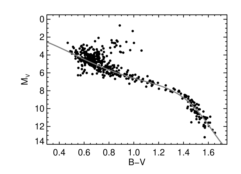
Figure 1: Color-magnitude diagram for the stars used in this work. The solid line is the fit to the main sequence used to determine $\Delta M_{\mbox{\scriptsize V}}$, the height above the main sequence.

represents the Hipparcos average main sequence where $a=\left\{\right.$1.11255, 5.79062, -16.76829, 76.47777,-140.08488, 127.38044, -49.71805, -8.24265, 14.07945, -3.43155$\left.\right\}$. Fig. 1 shows $M_{\mbox{\scriptsize V,MS}}$ plotted on a color-magnitude diagram with the stars from the sample described in 2.1. Evolved stars, lying above the main sequence, have positive values of $\Delta M_{\mbox{\scriptsize V}}$, while subdwarfs have negative values.

While a more appropriate metric might employ measured abundances to lift the degeneracy between the effects of metallicity and evolution on $\Delta M_{\mbox{\scriptsize V}}$, the goal here is to provide a description of radial velocity jitter without the benefit such measurements.

2.3 The Activity Metric

Active stars, especially active F dwarfs, exhibit higher levels of jitter than their inactive counterparts. To quantify this relationship, this work employs the activity metric $S$, as measured in Wright et al. (2004) for the Planet Search stars, which represents the amount of emission in the Ca II H and K line core normalized by nearby continuum regions. Wright et al. (2004), following Noyes et al. (1984), transformed $S$ to $R^{\prime}_{\mbox{\scriptsize HK}}$  which represents the fraction of a star’s total luminosity emitted by the chromosphere in the Ca II H and K lines. Example spectra containing Ca II H and K lines can be found in most of the planet discovery papers by the California and Carnegie Planet Search, e.g. Butler et al. (2003).

The quantity $R^{\prime}_{\mbox{\scriptsize HK}}$, however, is not well calibrated for stars with $\bv<0.4$ or $\bv>0.9$. To overcome this, this work employs an alternative metric of stellar activity, $F_{\mbox{\scriptsize{Ca~{}II}}}$, defined by Rutten (1984) (who used the expression “$F_{\mbox{\scriptsize{H}}}+F_{\mbox{\scriptsize{K}}}$” in that work) and described again in Rutten (1986). This metric differs from $R^{\prime}_{\mbox{\scriptsize HK}}$ primarily in that it does not correct for a photospheric component to the Ca II H and K lines and in that it is a flux density, rather than a fraction, since it is constructed using an additional factor of $T_{\mbox{\scriptsize eff}}^{4}$. Rutten & Schrijver (1987) argued that $F_{\mbox{\scriptsize{Ca~{}II}}}$ is a more appropriate metric for comparing activity levels among stars since it is related to soft X-ray and Mg II h and k fluxes by power laws with no color or luminosity dependence. Hall & Lockwood (1995) determined the units of $F_{\mbox{\scriptsize{Ca~{}II}}}$ to be $7.97\times 10^{5}\mbox{ erg}\mbox{ cm}^{-2}\mbox{s}^{-1}$. Rutten (1984) prescribes

$$F_{\mbox{\scriptsize{Ca~{}II}}}=SC_{\mbox{\scriptsize cf}}T_{\mbox{\scriptsize eff}}^{4}10^{-14}$$ (3)

to transform the $S$-values of the stars in the sample here to $F_{\mbox{\scriptsize{Ca~{}II}}}$ where

$$\log{C_{\mbox{\scriptsize cf}}}=0.25(\bv)^{3}-1.33(\bv)^{2}+0.43(\bv)+0.24$$ (4)

for main sequence stars with $0.3\leq\bv\leq 1.6$. This work takes $T_{\mbox{\scriptsize eff}}$ for sample stars from Valenti & Fischer (2005) or, for the few stars here without such measurements, from the $T_{\mbox{\scriptsize eff}}$-B Vrelation of Flower (1996).

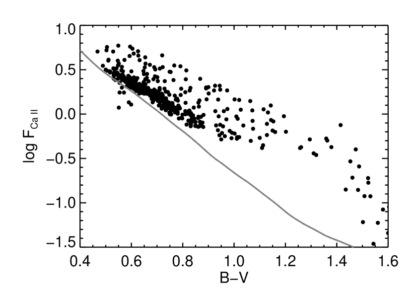
Figure 2: Activity, $F_{\mbox{\scriptsize{Ca~{}II}}}$, as a function of color for all of the stars used in this work. The solid line represents the minimum activity for dwarfs, $F_{\mbox{\scriptsize{Ca~{}II},min}}$.

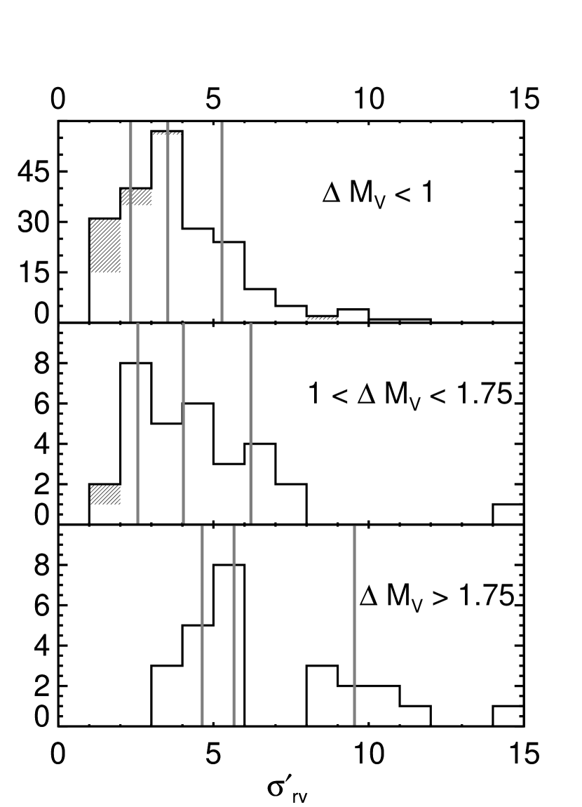
Figure 6: Distribution of $\sigma_{rv}^{\prime}$, the observed jitter, for inactive ($\Delta F_{\mbox{\scriptsize{Ca~{}II}}}<0.6$) stars in bins of $\Delta M_{\mbox{\scriptsize V}}$. The top panel includes only stars for which $0.6<\bv<1.4$, matching the majority of stars in the bottom two panels. Shaded regions indicate stars for which only upper limits on the jitter can be set.

Fig. 2 shows $F_{\mbox{\scriptsize{Ca~{}II}}}$ as a function of color for the sample stars here. Rutten (1987) tabulated the empirical minimum activity level $F_{\mbox{\scriptsize{Ca~{}II},min}}$ observed for stars as a function of B V. Table 1 and the solid line in Fig. 2 give this tabulation, converted to the units of this work. This minimum level ostensibly represents radiative flux not related to magnetic activity. A comparison of Fig. 2 with Fig. 6a of Rutten (1984) shows good agreement (note that the curves in Rutten’s figure have been superseded by the curves referenced above).

This work employs the activity metric $\Delta F_{\mbox{\scriptsize{Ca~{}II}}}$, constructed as:

$$\Delta F_{\mbox{\scriptsize{Ca~{}II}}}=F_{\mbox{\scriptsize{Ca~{}II}}}-F_{\mbox{\scriptsize{Ca~{}II},min}}$$ (5)

For some metal-poor, blue stars, $\Delta F_{\mbox{\scriptsize{Ca~{}II}}}$ is negative. Apparently, these stars’ very low metallicities ($[\mbox{Fe}/\mbox{H}]<-1$) require either a different calibration of $F_{\mbox{\scriptsize{Ca~{}II}}}$ or a different expression for $F_{\mbox{\scriptsize{Ca~{}II},min}}$ (or both). This is not a problem in this analysis, because, as described below, $\Delta F_{\mbox{\scriptsize{Ca~{}II}}}$ is not needed to predict the jitter for stars as inactive as these.

Table 1: The lower boundary of the surface flux $F_{\mbox{\scriptsize{Ca~{}II}}}$  as a function of B V, adapted from Rutten (1987) to the units of this work.

B V	$F_{\mbox{\scriptsize{Ca~{}II},min}}$
0.4	5.24
0.45	3.80
0.5	2.88
0.55	2.29
0.6	1.82
0.65	1.41
0.7	1.09
0.75	0.831
0.8	0.645
0.85	0.489
0.9	0.363
0.95	0.281
1.0	0.218
1.05	0.174
1.1	0.135
1.15	0.105
1.2	0.079
1.25	0.063
1.3	0.052
1.35	0.044
1.4	0.038
1.5	0.029
1.6	0.025

Henceforth, this work uses the term “active” to refer to stars with $F_{\mbox{\scriptsize{Ca~{}II}}}>0.6$. This limit corresponds to $\log{R^{\prime}_{\mbox{\scriptsize HK}}}\sim-4.95$ at $\bv=0.5$ and $\log{R^{\prime}_{\mbox{\scriptsize HK}}}\sim-4.8$ at $\bv=0.9$.

2.4 Radial Velocity Measurements

2.4.1 The Jitter Metric

Many sample stars exhibit linear trends in their radial velocity time series due to long-period planetary or stellar companions. To remove such effects, the standard deviation of the velocities, $\sigma_{rv}$ is defined about a linear trend, $v_{r}=a+bt$, for all of the time series:

$$\sigma_{rv}^{2}=\sum_{i=0}^{N}\frac{(v_{r,i}-a-bt_{i})^{2}}{N-2}$$ (6)

The quantity $\sigma_{rv}$ includes random measurement uncertainties such as those arising from photon statistics, estimated as follows. Each observation of a star consists of a spectrum divided into  400 chunks, each of which is analyzed independently the Planet Search Doppler analysis pipeline to determine the value of $\Delta v$, the differential radial velocity of the star with respect to a template observation. The distribution of the $\Delta v$ values of these 400 chunks provides an estimate of the measurement error for a given observation. Because the Planet Search employs an exposure meter at Keck, most observations of a given star have the same signal-to-noise (S/N) ratio, so the measurement errors for all observations of a given star are usually very similar. Thus, a single number $\sigma_{\mbox{\scriptsize meas}}$ provides an estimate of the contribution of measurement error to $\sigma_{rv}$ for observations of a given star.

Following Saar, Butler, & Marcy (1998), this work employs the metric $\sigma_{rv}^{\prime}\ =(\sigma_{rv}^{2}-\sigma_{\mbox{\scriptsize meas}}^{2})^{1/2}$ to quantify radial velocity variations in excess of $\sigma_{\mbox{\scriptsize meas}}$. The exposure meter at Keck ensures that those velocity errors limited by S/N are roughly constant across the sample, contributing 2-4 m$\mbox{s}^{-1}$to the error budget. The exceptions to this rule are faint M dwarfs, which receive a maximum of $\sim 10$ minutes per exposure and therefore have photon-limited errors of 3-8 m$\mbox{s}^{-1}$, and active F dwarfs that have high astrophysical jitter and receive short exposure times to keep errors photon-limited. For these stars, the observed rms velocities are nearly equal to $\sigma_{\mbox{\scriptsize meas}}$, indicating that photon statistics dominate the error budget. In cases in which where radial velocity variations in excess of $\sigma_{\mbox{\scriptsize meas}}$ remain undetected, this work simply assigns an upper limit of $\sigma_{\mbox{\scriptsize meas}}/2$:

$$\sigma_{rv}^{\prime}\left\{\begin{array}[]{ll}=\sqrt{\sigma_{rv}^{2}-\sigma_{\mbox{\scriptsize meas}}^{2}}&\sigma_{rv}^{2}>\frac{5}{4}\sigma_{\mbox{\scriptsize meas}}^{2}\\ \\ <\sigma_{\mbox{\scriptsize meas}}/2&\sigma_{rv}^{2}\leq\frac{5}{4}\sigma_{\mbox{\scriptsize meas}}^{2}\\ \end{array}\right.$$ (7)

2.4.2 The Components of $\sigma_{rv}^{\prime}$

In addition to astrophysical jitter, $\sigma_{rv}^{\prime}$ also measures undetected planetary companions and systematic errors as discussed below.

Many stars in this sample undoubtedly harbor still-undetected, low-amplitude planets. Only after many planetary orbits with good phase coverage can one use the periodic nature of the signals and Keplerian fits to distinguish these signals from jitter (Marcy et al., 2005). Refining these fits to determine the precise orbital elements of a planetary companion requires still more observations, and the statistics of the residuals to these fits is complex. It is for the sake of simplicity and uniformity in the sample that this work employs only linear fits to the velocity time series and not Keplerians.

Systematic errors have many sources, including imperfect deconvolution of template spectra (especially for M dwarfs) and poor charge transfer in the HIRES Tek CCD. The Planet Search estimates these errors to be on the order of 3 m$\mbox{s}^{-1}$for M dwarfs and $<2$ m$\mbox{s}^{-1}$for other stars (G. W. Marcy 2005, private communication). Some component of these systematic errors will be accounted for which the subtraction of $\sigma_{\mbox{\scriptsize meas}}$ from $\sigma_{rv}$, but systematic errors, by their nature, are not well characterized by Gaussian noise, so some component of these errors probably remain in $\sigma_{rv}^{\prime}$.

3 Analysis

The purpose of this paper is to quantify the known dependencies of radial velocity jitter on stellar parameters, namely that active, blue, and evolved stars exhibit more jitter than old, main sequence, G dwarfs. This section, therefore, discusses trends of jitter with respect to $\Delta F_{\mbox{\scriptsize{Ca~{}II}}}$, $\Delta M_{\mbox{\scriptsize V}}$, and B V.

3.1 Activity

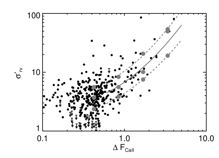
Figure 3: Activity, $\Delta F_{\mbox{\scriptsize{Ca~{}II}}}$, vs. the observed jitter, $\sigma_{rv}^{\prime}$ for stars with $\Delta M_{\mbox{\scriptsize V}}<1$. Typical errors on data points are around 1.5 m$\mbox{s}^{-1}$. Upper limits are represented by arrows. Large gray disks represent the 20th percentile, median, and 80th percentile in each of 4 equally spaced bins in $\log{\Delta F_{\mbox{\scriptsize{Ca~{}II}}}}$ from $0.3\leq\Delta F_{\mbox{\scriptsize{Ca~{}II}}}\leq 3$. The dashed lines represent the parabolic fits to these points in the range $0.6\leq\Delta F_{\mbox{\scriptsize{Ca~{}II}}}\leq 3$, where the model is applicable.

Fig. 3 shows $\sigma_{rv}^{\prime}$, as a function of $F_{\mbox{\scriptsize{Ca~{}II}}}$ for stars with $\Delta M_{\mbox{\scriptsize V}}<1$. There is a clear increase in $\sigma_{rv}^{\prime}$ with $F_{\mbox{\scriptsize{Ca~{}II}}}$, such that the most active stars consistently show more than 4 m$\mbox{s}^{-1}$of jitter. A few stars with $\Delta F_{\mbox{\scriptsize{Ca~{}II}}}<1$ appear to show more than $\sim 20$ m$\mbox{s}^{-1}$of jitter; these stars may harbor planets whose orbital periods have not yet become apparent from the radial velocity time series. However, two of these stars may be very young ($<1$ Gyr) according to Valenti & Fischer (2005), so one cannot discount the possibility that these $\sigma_{rv}^{\prime}$values are due purely to astrophysical jitter.

This work employs the following method to fit a polynomial to these data, which contain a few high outliers and points for which only an upper limit can be set. First, I divide the distribution into four evenly spaced bins in $\log{\Delta F_{\mbox{\scriptsize{Ca~{}II}}}}$. Within each bin I then find the median value, 20th percentile, and 80th percentile of $\sigma_{rv}^{\prime}$ (represented by large gray filled circles in Fig. 3), yielding three sets of points to which I fit second-order polynomials. In Figure 3, dashed lines represent the fits to the 20th and 80th percentile points, and the solid line represents the avereage of these fits, representing the model of the median. The Appendix describes the definition of a median and a percentile in a data set containing upper limits. Note that the choice of a second-order polynomial here is not physically or statistically motivated, but is merely chosen to be a simple, accurate description of the distribution with a smooth transition to the low-activity subsample.

There is very little change in the median jitter for stars with $\Delta F_{\mbox{\scriptsize{Ca~{}II}}}<0.6$, so these fits are only applicable for stars with $\Delta F_{\mbox{\scriptsize{Ca~{}II}}}>0.6$. Of the 72 such stars in the sample, 53% lie below the solid line in Fig. 3, 80% lie below the 80th percentile fit, and 20% lie below the 20th percentile fit. Table 2 contains coefficients for these polynomials.

The result here, that jitter increases with activity is consistent with the result of Saar et al. (2003), who found $\sigma_{rv}^{\prime}\propto(R^{\prime}_{\mbox{\scriptsize HK}})^{b}$, with $b=1.1$ for G and K dwarfs and $b=1.7$ for F dwarfs. Although here the fit is parabolic and is applied to a different metric, one can compare the results by fitting a line to $\sigma_{rv}^{\prime}$ versus $\log{R^{\prime}_{\mbox{\scriptsize HK}}}$ for the F stars and the G and K stars separately, using the ASURV statistical analysis package rev 1.2 Lavalley, Isobe, & Feigelson (1992), which implements the methods presented in Isobe, Feigelson, & Nelson (1986) to handle the upper limits. The best-fit values for found $b$ by applying the Buckley-James method and the parametric EM algorithm are $b=1.6$ for F dwarfs ($\bv<0.63$,$\Delta M_{\mbox{\scriptsize V}}<1$) and $b=0.80$ for G and K dwarfs ($0.63<\bv<1.4$, $\Delta M_{\mbox{\scriptsize V}}<1$). While these results differ somewhat from the results of Saar et al., the strong color dependence remains.

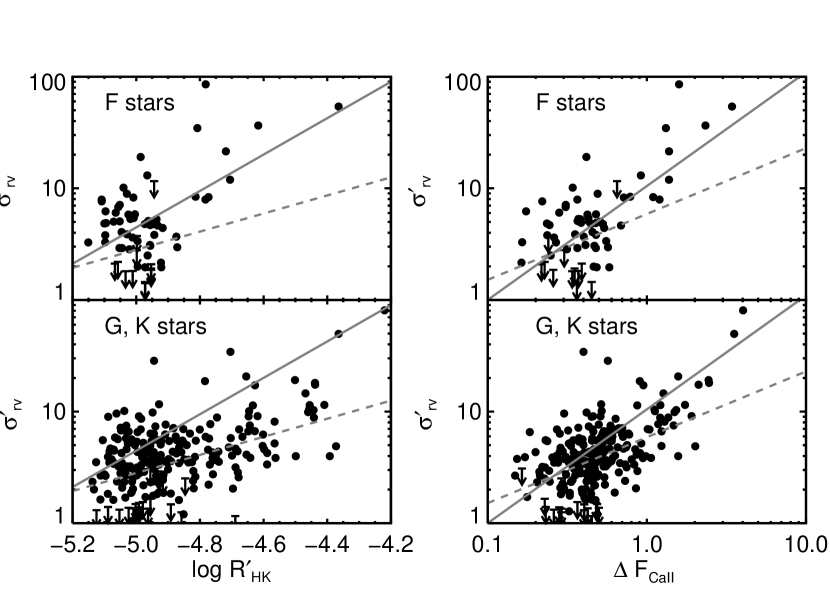
Figure 4: Jitter as a function of activity using two different activity metrics. Solid lines represent fits using only F stars, dashed lines those using only the G and K stars. F stars show a steeper activity dependence than G and K stars with $\log{R^{\prime}_{\mbox{\scriptsize HK}}}$ as a metric (left panel), but the difference is smaller when $F_{\mbox{\scriptsize{Ca~{}II}}}$ is the metric (right panel). These fits are provided for comparison only, and are not used in the jitter model presented here.

However, using the activity metric $\Delta F_{\mbox{\scriptsize{Ca~{}II}}}$ instead, however, with its extra factor of $T_{\mbox{\scriptsize eff}}^{4}$, this color dependence is somwhat reduced: a similar fit to the relation $\sigma_{rv}^{\prime}\propto(\log{\Delta F_{\mbox{\scriptsize{Ca~{}II}}}})^{c}$ returns $c=0.59$ for G and K dwarfs and $c=1.01$ for F dwarfs. The choice of $\Delta F_{\mbox{\scriptsize{Ca~{}II}}}$ thus reduces the color dependence of the jitter-activity relation, as shown in Fig. 4.

3.2 Stellar Evolution

Fig. 5 shows $\sigma_{rv}^{\prime}$, as a function of $\Delta M_{\mbox{\scriptsize V}}$ for stars with $\Delta F_{\mbox{\scriptsize{Ca~{}II}}}<0.6$. Stars with $\Delta M_{\mbox{\scriptsize V}}>2$ have higher typical $\sigma_{rv}^{\prime}$-values than stars on the main sequence. The trend here is weak, so in this case, the model consists of three broad groups, each modeled independently: main-sequence stars ($\Delta M_{\mbox{\scriptsize V}}<1$), slightly evolved stars ($1<\Delta M_{\mbox{\scriptsize V}}<1.75$), and subgiants ($\Delta M_{\mbox{\scriptsize V}}>1.75$).

Fig. 6 shows the distribution of $\sigma_{rv}^{\prime}$ values for these three bins in $\Delta M_{\mbox{\scriptsize V}}$, with shaded regions representing those stars for with $\sigma_{rv}^{\prime}$ exceeds $\sigma_{\mbox{\scriptsize meas}}/2$ (that is, upper limits on $\sigma_{rv}^{\prime}$) (Eq. 7). The median, 20th, and 80th percentile levels for these distributions appear as vertical gray bars in Fig. 6, and numerically in Table 2. Again, the appendix describes the statistics of medians for these data sets.

Fig. 6 shows that subgiants exhibit higher $\sigma_{rv}^{\prime}$ values than their main-sequence counterparts, having a median $\sigma_{rv}^{\prime}$ value $>5$m$\mbox{s}^{-1}$, significantly higher than the non-astrophysical sources of noise discussed in § 2.4.2. In fact, no subgiant in the sample performs better than 3 m$\mbox{s}^{-1}$. These stars are therefore poor velocity standards, due to jitter.

The distribution of slightly evolved stars is very similar to that of main sequence stars. This work nonetheless treats them separately here, because their activity levels, normally a good indicator of jitter, are generally lower and therefore not comparable to main-sequence stars (Wright, 2004). Their numbers are too few for further subdivisions into bins of color or activity, so the model given here simply incorporates median $\sigma_{rv}^{\prime}$ values for this group as a whole.

3.3 Color

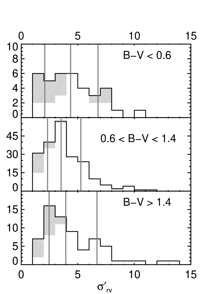
Figure 7: Distribution of $\sigma_{rv}^{\prime}$, the observed jitter, for inactive ($\Delta F_{\mbox{\scriptsize{Ca~{}II}}}<0.6$), unevolved ($\Delta M_{\mbox{\scriptsize V}}<1$) stars in three color bins. The intermediate color stars show the lowest median jitter. Shaded regions indicate stars for which only upper limits on the jitter can be set.

Fig. 7 shows the distribution of $\sigma_{rv}^{\prime}$ values for stars in three B V ranges (corresponding roughly to spectral types F, G and K, and M) that have $\Delta M_{\mbox{\scriptsize V}}<1$ and $F_{\mbox{\scriptsize{Ca~{}II}}}<0.6$. Here again, vertical bars show the values of the 20th percentile, median, and 80th percentile, and shaded regions represent upper limits.

Jitter in these unevolved inactive stars is not a well-determined, smooth function of color, but, broadly speaking, three distinct B V groups exist. Blue stars ($\bv<0.6$) generally show $\sim 5$ m$\mbox{s}^{-1}$of jitter, while G and K dwarfs exhibit a median $\sigma_{rv}^{\prime}$ value of 3 m$\mbox{s}^{-1}$. The large number of shaded stars in the distribution of F stars in Fig. 7 reflects the fact that, as noted in § 2.1, Planet Search stars do not receive more exposure time than their jitter levels warrant, to keep errors photon-limited. Note that this practice does not artificially inflate the estimate of jitter in these stars because the method of calculating medians accounts for these upper limits (Appendix).

The $\sigma_{rv}^{\prime}$ distribution of M dwarfs exhibits a tail of high jitter values ($\sigma_{rv}^{\prime}\sim$ 7 m$\mbox{s}^{-1}$), which most likely represents systematic errors in the deconvolution of their spectra, made difficult by the lack of continuum in such cool stars. The large shaded regions of the M dwarf distribution are due to these stars’ faintness: as noted in § 2.1, no Planet Search star receives more than 10 minutes of exposure at a time, so faint M dwarfs will yield lower S/N ratios and thus have photon-limited precision.

G and K dwarfs yield the best radial-velocity performance, with over 30 members exhibiting rms velocities below 2 m$\mbox{s}^{-1}$. It is fortunate that the best performing stars in the sample are those that most closely resemble the Sun.

Table 2: Jitter values for different regions in $\Delta F_{\mbox{\scriptsize{Ca~{}II}}}$, B V, $\Delta M_{\mbox{\scriptsize V}}$ space. Values in curly braces are coefficients in a polynomial fit: for an entry $\{a_{0},a_{1},a_{2}\}$, $\log{\sigma_{rv}^{\prime}}=\sum_{i}a_{i}(\bv)^{i}$.

Region			$\sigma_{rv}^{\prime}$(m$\mbox{s}^{-1}$)
$\Delta M_{\mbox{\scriptsize V}}$	$\Delta F_{\mbox{\scriptsize{Ca~{}II}}}$	B V	20th percentile	median	80th percentile
$1.75<\Delta M_{\mbox{\scriptsize V}}<4$	$<0.6$	$\cdots$	4.6	5.7	9.5
$1<\Delta M_{\mbox{\scriptsize V}}<1.75$	$<0.6$	$\cdots$	2.6	4.0	6.2
$<1$	$0.6\leq\Delta F_{\mbox{\scriptsize{Ca~{}II}}}<3$	$\bv<1.4$	$\{0.64,0.92,0.55\}$	$\{0.83,0.96,0.61\}$	$\{1.02,1.01,0.68\}$
$<1$	$<0.6$	$<0.6$	2.1	4.4	6.8
$<1$	$<0.6$	$0.6<\bv<1.4$	2.3	3.5	5.3
$<1$	$<0.6$	$>1.4$	2.5	3.9	6.7

3.4 Other Regions

Stars that are both active and either evolved or very red ($\bv>1.4$) are not discussed here, because there are too few sample stars to properly determine the behavior of such stars.

Only two sample stars meet the criteria for study here (§ 2.1) and have $\Delta F_{\mbox{\scriptsize{Ca~{}II}}}>0.6$ and $\bv>1.4$. They have $\sigma_{rv}^{\prime}$ values of 20 and 11 m$\mbox{s}^{-1}$, both higher than the values predicted by the median curve in Fig. 3, which are $\sim 5$ m$\mbox{s}^{-1}$. This indicates that red, active stars may have substantially more jitter than their bluer or more-inactive counterparts.

The region of $\Delta F_{\mbox{\scriptsize{Ca~{}II}}}$-$\Delta M_{\mbox{\scriptsize V}}$ space corresponding to active ($\Delta F_{\mbox{\scriptsize{Ca~{}II}}}>0.6$), evolved ($\Delta M_{\mbox{\scriptsize V}}>1$) stars is poorly populated, not just in this sample, but also in other surveys of Sun like stars (Wright, 2004). The sole such star in this sample has $\sigma_{rv}^{\prime}=21$ m$\mbox{s}^{-1}$, substantially higher than the 6 m$\mbox{s}^{-1}$predicted by the $\sigma_{rv}^{\prime}$-activity relation here. Such stars often represent massive early F stars that have entered or are entering the subgiant phase before losing substantial amounts of angular momentum (do Nascimento et al., 2003).

4 The Jitter Model

Table 2 contains the $\sigma_{rv}^{\prime}$ values that are typical for various regions given in (B V)-$F_{\mbox{\scriptsize{Ca~{}II}}}$-$\Delta M_{\mbox{\scriptsize V}}$ space. The jitter model assumes that a given star will exhibit levels of jitter similar to those of other stars in its region. When the Planet Search pipeline fits Keplerian orbits to radial velocity time series, it incorporates the jitter-model estimate of the jitter into its estimate of the errors. Furthermore, the model also consists of interpreting the median values in the appropriate region of Table 2 as the estimated jitter, but with the following minor modifications.

To prevent large discontinuities in the jitter model, the model linearly interpolates the median jitter for stars within 0.1 mag of the B V boundaries. For instance, an unevolved, inactive star with $\bv=0.65$ would have predicted jitter of 3.725 m$\mbox{s}^{-1}$: since it is within 0.1 mag of the boundary between the fourth and fifth entries in Table 2, the model interpolates between the median value for the $\bv<0.6$ and $0.6<\bv<1.4$ regions. The model also similarly interpolates between the first and second regions of Table 2 for stars with $1.65<\Delta M_{\mbox{\scriptsize V}}<1.85$. The model also sets the predicted jitter of active stars ($F_{\mbox{\scriptsize{Ca~{}II}}}>0.6$) to the greater of the predicted jitter and that predicted for an inactive star with the same B V and $M_{\mbox{\scriptsize V}}$.

Both this jitter model and the regions and values in Table 2 have evolved and become more sophisticated over time, so the model described here may not agree precisely with jitter estimates published in previous work by the California and Carnegie Planet Search.

This model is generally applicable for most Planet Search stars. Since it was derived using Keck data, in particular data before the September 2004 upgrade of the HIRES CCD, it accounts for systematic errors that may not be present in radial velocity data from other telescopes. For jitter values $>3$m$\mbox{s}^{-1}$, however, it predominantly measures astrophysical jitter, and so is generally applicable. The presence of undetected planets around the sample stars means that these values may be slightly overestimated, but the use of medians mitigates this effect.

Jitter is more important to the detection of exoplanets than the characterization of their orbits. The effects of including jitter in one’s noise estimate on best-fit orbital parameters for a single-planet system are generally very small ($<1\%$), in part because the errors are typically already nearly equal. Jitter plays a more important role in determining whether radial velocity variations are of stellar or Keplerian origin. To the extent that the jitter measured here is astrophysical and not due to systematics or still-undetected planets, the $2-5$ m $\mbox{s}^{-1}$of jitter exhibited by most inactive stars represents a minimum detection threshold below which planets will be very difficult to detect.

5 Conclusions

This work concerns a sample of the California and Carnegie Planet Search data stars representing stars without obvious or detected planets observed at the Keck Observatory. This sample describes the typical radial velocity stability, measured as $\sigma_{rv}^{\prime}$, of most stars in the Planet Search. The metric $\sigma_{rv}^{\prime}$ includes the effects of undetected planets, systematic errors ($\lesssim 3$m$\mbox{s}^{-1}$), and astrophysical jitter.

Among inactive stars F, G and K, and M dwarfs show sightly different amounts of radial velocity jitter, from 3.5 m$\mbox{s}^{-1}$for G and K dwarfs to nearly 5 m$\mbox{s}^{-1}$for M dwarfs. Evolved stars ($\Delta M_{\mbox{\scriptsize V}}>1.75$) show significant amounts of jitter, while those only slightly evolved appear more consistent with main sequence stars.

Active stars show markedly more jitter ($5-10$ m $\mbox{s}^{-1}$) than inactive stars, and this jitter increases with activity. The activity metric $F_{\mbox{\scriptsize{Ca~{}II}}}$ of Rutten can provide an estimate of jitter without the strong color dependence of previous models that employed $R^{\prime}_{\mbox{\scriptsize HK}}$ as a metric.

Appendix A Medians and Percentiles of Data Sets That Include Limits

The median is defined as the $N/2$th largest element of a sorted $N$-element data set. The presence of measurements for which one can only set limits (nondetections, for instance) complicates matters somewhat, but a median can still be similarly defined.

Consider a sorted $N$-element data set $x$, comprising elements $x_{i}$ where $0\leq i<N$. Each $x_{i}$ represents a measurement that is either exact (a data point), an upper limit, or a lower limit. The set $x$ should be sorted such that for otherwise equal elements, an upper limit is less than a data point, which in turn is less than a lower limit. (Note that these definitions apply only to the sorting procedure; different comparison conditions apply below.) One seeks to test the value of each element $x_{i}$ as a candidate median by comparing $a_{i}$, the number of elements unambiguously above the value of $x_{i}$, to $b_{i}$, the number unambiguously below it.

For the purposes of computing $b_{i}$, element $x_{j}$ is counted as being below the value of $x_{i}$ if, in the sorted array: (1) $x_{j}$ is a data point and $j<i$ or (2) $x_{j}$ is an upper limit and $j\leq i$. Note that when $x_{i}$ represents an upper limit, $x_{i}$ is less than the value of $x_{i}$ by definition, and so contributes to $b_{i}$, and that when $x_{j}$ represents a lower limit, it does not contribute to $b_{i}$ at all. Similarly, $x_{j}$ contributes to $a_{i}$ if $j>i$ when $x_{j}$ is a data point, or if $j\geq i$ when $x_{j}$ is a lower limit.

The median is then is the value of the $i$th element of $x$ such that $a_{i}$ is most nearly equal to $b_{i}$. If more than one such element exists, these can simply be averaged. In some cases, such as a data set consisting entirely of upper limits, no median can be defined. Similarly, the $p$th percentile can be defined as the value of $x_{i}$ such that $b_{i}/(a_{i}+b_{i})$ is most nearly $p/100$. Naturally, the 50th percentile is equivalent to the median.

For example, consider the appropriately sorted data set $x=\{<1,5,5,<7,10,50\}$, in which the first and fourth elements represent upper limits. The values of $a$ for this set are $\{4,3,2,2,1,0\}$, and similarly $b=\{1,1,2,4,4,5\}$. Thus, the median of this set is 5 ($=x_{2}$, since $a_{2}=b_{2}$), the 20th percentile is 1 ($=x_{0}$, since $b_{0}/(a_{0}+b_{0})=1/5=p/100$ when $p=20$), and the 80th percentile is 10 ($=x_{4}$, since $b_{4}/(a_{4}+b_{4})=4/5=p/100$ when $p=80$).

Figure 5: Evolution, measured as $\Delta M_{\mbox{\scriptsize V}}$ vs. $\sigma_{rv}^{\prime}$, for stars with $F_{\mbox{\scriptsize{Ca~{}II}}}<0.6$. Typical errors on data points are around 1.5 m$\mbox{s}^{-1}$. Arrows represent upper limits. The most evolved stars exhibit large amounts of jitter.

References

- Butler et al. (2003) Butler, R. P., Marcy, G. W., Vogt, S. S., Fischer, D. A., Henry, G. W., Laughlin, G., & Wright, J. T. 2003, ApJ, 582, 455
- do Nascimento et al. (2003) do Nascimento, J. D., Canto Martins, B. L., Melo, C. H. F., Porto de Mello, G., & De Medeiros, J. R. 2003, A&A, 405, 723
- ESA (1997) ESA 1997, The Hipparcos and Tycho catalogues, ESA SP-1200
- Flower (1996) Flower, P. J. 1996, ApJ, 469, 355
- Hall & Lockwood (1995) Hall, J. C. & Lockwood, G. W. 1995, ApJ, 438, 404
- Henry, Donahue, & Baliunas (2002) Henry, G. W., Donahue, R. A., & Baliunas, S. L. 2002, ApJ, 577, L111
- Isobe, Feigelson, & Nelson (1986) Isobe, T., Feigelson, E. D., & Nelson, P. I. 1986, ApJ, 306, 490
- Lavalley, Isobe, & Feigelson (1992) Lavalley, M., Isobe, T., & Feigelson, E. 1992, Astronomical Society of the Pacific Conference Series, 25, 245
- Marcy et al. (2005) Marcy, G. W., Butler, R. P., Vogt, S. S., Fischer, D. A., Henry, G. W., Laughlin, G., Wright, J. T., & Johnson, J. A. 2005, ApJ, 619, 570
- Noyes et al. (1984) Noyes, R. W., Hartmann, L. W., Baliunas, S. L., Duncan, D. K., & Vaughan, A. H. 1984, ApJ, 279, 763
- Paulson, Cochran, & Hatzes (2004) Paulson, D. B., Cochran, W. D., & Hatzes, A. P. 2004, AJ, 127, 3579
- Queloz et al. (2001) Queloz, D., et al. 2001, A&A, 379, 279
- Rutten (1984) Rutten, R. G. M. 1984, A&A, 130, 353
- Rutten (1986) Rutten, R. G. M. 1986, A&A, 159, 291
- Rutten (1987) Rutten, R. G. M. 1987, A&A, 177, 131
- Rutten & Schrijver (1987) Rutten, R. G. M. & Schrijver, C. J. 1987, A&A, 177, 155
- Saar & Donahue (1997) Saar, S. H., & Donahue, R. A. 1997, ApJ, 485, 319
- Saar, Butler, & Marcy (1998) Saar, S. H., Butler, R. P., & Marcy, G. W. 1998, ApJ, 498, L153
- Saar et al. (2003) Saar, S. H., Hatzes, A., Cochran, W., & Paulson, D. 2003, The Future of Cool-Star Astrophysics: 12th Cambridge Workshop on Cool Stars, Stellar Systems, and the Sun (2001 July 30 - August 3), eds. A. Brown, G.M. Harper, and T.R. Ayres, (University of Colorado), 12, 694
- Santos et al. (2003) Santos, N. C., et al. 2003, A&A, 406, 373
- Valenti & Fischer (2005) Fischer, D. A., Valenti, J. A 2005, ApJS, accepted
- Wright et al. (2004) Wright, J. T., Marcy, G. W., Butler, R. P., & Vogt, S. S. 2004, ApJS, 152, 261
- Wright (2004) Wright, J T. 2004, AJ, 128