Inflationary Solutions in Nonminimally Coupled Scalar Field Theory

Abstract

We study analytically and numerically the inflationary solutions for various type scalar potentials in the nonminimally coupled scalar field theory. The Hamilton-Jacobi equation is used to deal with nonlinear evolutions of inhomogeneous spacetimes and the long-wavelength approximation is employed. The constraints that lead to a sufficient inflation are found for the nonminimal coupling constant and initial conditions of the scalar field for inflation potentials. In particular, we numerically find an inflationary solution in the new inflation model of a nonminimal scalar field.

I Introduction

The origin of the large scale structure could be well explained in the inflationary scenario which predicts a scale invariant spectrum, Gaussian statistics, and the curvature perturbation. However, a recent attention on the non-Gaussianity of the temperature anisotropy maldacena03 has motivated the investigation of the gravitational perturbations during an inflation period beyond the linear order theory. The Hamilton-Jacobi theory, for instance, has been used to study nonlinear evolutions of inhomogeneous spacetimes in Einstein gravity salopek90 and generalized gravity soda95 ; koh05 . Even though it is difficult to get exact solutions of the Hamilton-Jacobi equation, the long-wavelength approximation is useful in dealing with superhorizon size perturbations. When the scale of perturbations is larger than the horizon size, spatial gradient terms can be neglected compared to their temporal variations. In this sense, the lowest order Hamilton-Jacobi and evolution equations for fields look like homogeneous equations of motion in the long-wavelength approximation.

Inflation potentials that dominate the energy density during the inflation period, are a crucial ingredient to discriminate among different inflation models. In Ref. lidsey97 , the inflation potentials were reconstructed from observational data. The inflation models can be classified according to the shape of the potential and the initial condition of the scalar field into three types: a large field, small field and hybrid field model dodelson97 . The chaotic inflation linde83 , which belongs to the large field model, has a positive curvature at the minimum of the potential and needs the initial condition $\phi_{0}>m_{pl}$ to result in a sufficient inflation. Contrary to the chaotic inflation, the new inflation linde82 (a small field model) has a negative curvature at the false vacuum and requires $\phi_{0}\ll m_{pl}$. The scalar field in the new inflation starts from the false vacuum initially and then rolls down to the true vacuum. And the hybrid inflation linde91 ; copeland94 has a positive curvature at the local minimum of the potential but has a non-zero energy which is different from the chaotic inflation model. One of the interesting features of the hybrid inflation is prediction of a blue power spectrum ($n>1$, $n$ being a spectral index) when perturbation modes leave the horizon.

The Brans-Dicke-like theories are naturally derived from the fundamental physics theory such as string or M-theory. They are also widely used to investigate the dark energy problem that is believed to be responsible for the present accelerating Universe. When the scalar fields are coupled to the spacetime curvature $R$ through $\xi R\phi^{2}/2$, the theory is renormalizable. The inflationary solutions were investigated in this nonminimally coupled scalar field theory and constraints on the nonminimal coupling constant $\xi$ were found futamase89 ; fakir90 ; tsujikawa00 . But many of models considered there are the chaotic inflation. The coupling term might prevent inflation from occurring in the new inflation model abbott81 because it behaves like a mass term in the scalar potential and destroys the flatness of the potential.

In this paper we try to find inflationary solutions in the nonminimally coupled scalar field theory for various potentials and use the Hamilton-Jacobi theory to deal with nonlinear evolutions of inhomogeneous spacetimes. Although the inflationary solutions in the new inflation model are believed to be impossible, we try to get the inflationary solutions by numerical calculations and the slow-roll approximation in the new inflation. We also find analytically or numerically the inflationary solutions for chaotic and hybrid inflation models and put constraints on the nonminimal coupling constant.

This paper is organized as follows. In. Sec. II, we derive the Hamilton-Jacobi and evolution equations for the gravitation and scalar fields when the scalar field is nonminimally coupled to the gravity. And then we solve the Hamilton-Jacobi equation approximately using slow-roll conditions during the inflation period in Sec. III. We consider the inflation potentials in chaotic, new, and hybrid inflation models. To compare with approximate analytical solutions, we perform numerical calculations in Sec. IV and finally we summarize our results in Sec. V.

II Hamilton-Jacobi Equation in Nonminimally Coupled Scalar Field Theory

The action for a nonminimally coupled scalar field takes the form

$$\mathcal{I}=\int d^{4}x\sqrt{-g}\left[(1-8\pi G\xi\phi^{2})\frac{R}{16\pi G}-\frac{1}{2}g^{\mu\nu}\partial_{\mu}\phi\partial_{\nu}\phi-V(\phi)\right],$$ (1)

where $\xi$ is a nonminimal coupling constant. The action (1) may be interpreted to have an effective gravitational constant $G_{eff}$ depending on the scalar field as futamase89

$$G_{eff}=\frac{G}{1-\phi^{2}/\phi_{c}^{2}},$$ (2)

where

$$\phi_{c}^{2}=\frac{1}{8\pi G\xi}\equiv\frac{m_{pl}^{2}}{8\pi\xi}.$$ (3)

We will require $G_{eff}>0$ to relate to our present Universe, and thus we restrict $\phi$ to the region $\phi<\phi_{c}$ for $\xi>0$. In the Hamilton-Jacobi formalism, the spacetime is written in the ADM metric

$$ds^{2}=-N^{2}dt^{2}+\gamma_{ij}dx^{i}dx^{j},$$ (4)

where $N$ and $\gamma_{ij}$ are a lapse function and a 3-spatial metric and we set a shift vector $N^{i}=0$.

The Hamilton-Jacobi theory proves useful for solving the gravitational and scalar field equations which can be obtained from the variation of the action (1). By introducing a generating functional $S$ that is a function of $\gamma_{ij},\phi$ and integration constants, we can get the Hamilton-Jacobi and momentum constraint equations salopek90 ; koh05 . The generating functional, $S(\phi,\gamma_{ij})$, can be expanded in a series in the order of spatial gradient terms

$$S=S^{(0)}+S^{(2)}+S^{(4)}+\cdots.$$ (5)

The lowest order Hamilton-Jacobi equation is sufficient to deal with the nonlinear evolution of the gravitational fields whose scales are larger than the horizon size. We will assume an ansatz for the lowest order generating functional of the form koh05

$$S^{(0)}(\phi,\gamma_{ij})=-\frac{1}{4\pi G}\int d^{3}x\gamma^{1/2}(1-8\pi G\xi\phi^{2})^{3/2}W(\phi,\gamma_{ij}),$$ (6)

so that $S^{(0)}$ satisfies automatically the momentum constraint equation. For Einstein gravity, $W$ can be interpreted as a locally defined Hubble parameter. Then the Hamilton-Jacobi and evolution equations for $\gamma_{ij}$ and $\phi$ are given by

$$W^{2}-\frac{4\pi G(1-8\pi G\xi\phi^{2}(1-6\xi))}{3(1-8\pi G\xi\phi^{2})^{3}}\left(\frac{1}{N}\dot{\phi}\right)^{2}-\frac{8\pi G}{3(1-8\pi G\xi\phi^{2})^{2}}V=0,$$ (7)

$$\frac{1}{N}\dot{\alpha}\equiv H=\sqrt{1-8\pi G\xi\phi^{2}}\left[W+\frac{8\pi G\xi\phi}{(1-8\pi G\xi\phi^{2})^{3/2}}\frac{1}{N}\dot{\phi}\right],$$ (8)

$$\frac{1}{N}\dot{\phi}=-\frac{(1-8\pi G\xi\phi^{2})^{5/2}}{4\pi G(1-8\pi G\xi\phi^{2}(1-6\xi))}W_{\phi},$$ (9)

where the metric is factored into a conformal part and a unimodular metric

$$\gamma_{ij}(t,{\bf x})=e^{2\alpha(t,{\bf x})}h_{ij}({\bf x}),\quad\det(h_{ij})=1.$$ (10)

There appears another singular point $\phi=\phi_{s}$ from Eq. (9) in the case $0<\xi<1/6$, where

$$\phi_{s}=\frac{m_{pl}}{\sqrt{8\pi\xi(1-6\xi)}}=\frac{\phi_{c}}{\sqrt{1-6\xi}}.$$ (11)

Note that Eq. (7) can also be written as

$$\left(H-\frac{\phi}{\phi_{c}^{2}-\phi^{2}}\frac{1}{N}\dot{\phi}\right)^{2}-\frac{\phi_{c}^{2}(\phi_{s}^{2}-\phi^{2})}{6\xi\phi_{s}^{2}(\phi_{c}^{2}-\phi^{2})^{2}}\left(\frac{1}{N}\dot{\phi}\right)^{2}-\frac{1}{3\xi(\phi_{c}^{2}-\phi^{2})}V=0.$$ (12)

There is no stable solution for $\phi>\phi_{s}$ in an isotropic flat spacetime futamase89 . This can be understood because each term in Eq. (12) becomes positive definite if $\phi>\phi_{s}(>\phi_{c})$. Thus the Hamiltonian constraint cannot be not satisfied for $\phi>\phi_{s}$.

III Slow-roll approximation

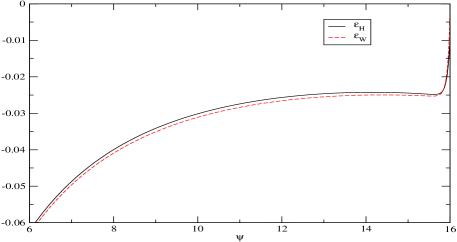
Figure 1: Comparison of $\varepsilon_{H}$ and $\varepsilon_{W}$ during an inflation period for $V=m^{2}\phi^{2}/2$. Here $\psi\equiv\sqrt{8\pi G}\phi$ and we set $\psi_{0}=16$ and $\xi=10^{-3}$.

Although the Hamilton-Jacobi method is a powerful tool for nonlinear evolutions of inhomogeneous spacetimes, it is known to be difficult to solve exactly the Hamilton-Jacobi equation for a general potential even in Einstein gravity salopek90 . In Ref. koh05 for generalized gravity, the Hamilton-Jacobi equation is analytically solved for general potentials using some approximate methods. A good approximation is the slow-roll approximation in inflation scenario to get analytical results which are well fitted to observations. We will try to get an analytical result of Eq. (7) using the slow-roll approximation.

The slow-roll conditions during the inflation period are

$$\frac{1}{2}\dot{\phi}^{2}\ll V(\phi),\quad\ddot{\phi}\ll 3H\dot{\phi}.$$ (13)

It turns out convenient to define slow-roll parameters from the above slow-roll conditions

$$\varepsilon_{H} \equiv \frac{\dot{H}}{NH^{2}}=\frac{\dot{\phi}}{N}\frac{H_{,\phi}}{H^{2}},\quad\eta_{H}\equiv\frac{1}{N}\left(\frac{\dot{\phi}}{N}\right)^{\cdot}\frac{N}{H\dot{\phi}},$$ (14)

$$\varepsilon_{W} \equiv \frac{\dot{W}}{NW^{2}}=\frac{\dot{\phi}}{N}\frac{W_{,\phi}}{W^{2}},\quad\eta_{W}\equiv\frac{1}{N}\left(\frac{\dot{\phi}}{N}\right)^{\cdot}\frac{N}{W\dot{\phi}}.$$ (15)

Here $\varepsilon_{H}$ and $\eta_{H}$ are usual definitions of slow-roll parameters, and $\varepsilon_{H}$ and $\varepsilon_{W}$ are related to each other

$$\varepsilon_{H}=\frac{\varepsilon_{W}}{\sqrt{1-8\pi G\xi\phi^{2}}}+\frac{2\xi\phi(1-8\pi G\xi\phi^{2})}{1-8\pi G\xi\phi^{2}(1-6\xi)}\frac{W_{,\phi}}{W}.$$ (16)

The occurrence of inflation requires $\varepsilon_{H},\eta_{H}\ll 1$. In Fig. 1, $\varepsilon_{H}$ and $\varepsilon_{W}$ are plotted for $V=m^{2}\phi^{2}/2$ during the inflation period. $\varepsilon_{H}$ and $\varepsilon_{W}$ are slightly different from each other, but they are both useful in determining the end of inflation, $\varepsilon_{H}\simeq\varepsilon_{W}=1$.

From Eq. (7), unless $|\xi|$ is much larger than $1$, the slow-roll condition is equivalent to neglecting the kinetic energy term in comparison to the potential energy. Then the Hamilton-Jacobi equation and the evolution equation for $\alpha$ become approximately

$$W^{2} \simeq \frac{8\pi G}{3(1-8\pi G\xi\phi^{2})^{2}}V,$$ (17)

$$\frac{1}{N}\dot{\alpha} \simeq \sqrt{1-8\pi G\xi\phi^{2}}W.$$ (18)

Another useful quantity to describe a sufficient inflation is the number of $e$-folds, $\mathcal{N}$, which is defined by

$$\mathcal{N}=\int^{\alpha_{e}}_{\alpha_{0}}d\alpha=\alpha(\phi_{e})-\alpha(\phi_{0})=\int^{\phi_{e}}_{\phi_{0}}\frac{H}{\dot{\phi}/N}d\phi,$$ (19)

where subscripts “$e$” denotes the end of inflation. To resolve the cosmological problems such as the flatness, horizon, and homogeneity problems, a bound $\mathcal{N}\gtrsim 60$ is required. With the help of Eqs. (18) and (9), $\mathcal{N}$ can be written as

$$\mathcal{N}=-4\pi G\int^{\phi_{e}}_{\phi}\frac{1-8\pi G\xi\phi^{2}(1-6\xi)}{(1-8\pi G\xi\phi^{2})^{2}}\frac{W}{W_{,\phi}}d\phi.$$ (20)

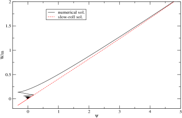
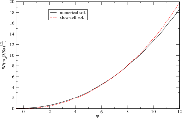
Figure 2: Comparison of slow-roll solutions with numerical solutions for $V=m^{2}\phi^{2}/2$ (left panel) and for $V=\lambda\phi^{4}/4!$ (right panel).

We will solve the Hamilton-Jacobi equation for various type potentials using the slow-roll approximation and find initial conditions for the scalar field to result in a sufficiently enough inflation. According to Ref. dodelson97 , inflation potentials in a single field model are classified into three types depending on the shape of potentials and the initial condition of the scalar field - a large field, small field and hybrid field model. In the large field model, for example in the chaotic inflation, the scalar field that is initially greater than $m_{pl}$ rolls slowly down to the minimum and then oscillates around the minimum value. And the potential has a positive curvature at the minimum. Contrary to the large field model, the scalar field in the small field model such as the new inflation stays initially near a false vacuum and then evolves toward the true vacuum. So it is possible to have an inflation even when the field is much smaller than $m_{pl}$ and the potential at the minimum has a negative curvature. And finally the scalar field in the hybrid inflation evolves toward a minimum of the potential which has a nonzero vacuum energy.

III.1 A large field model, $V(\phi)\propto\phi^{p}$

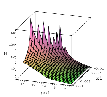
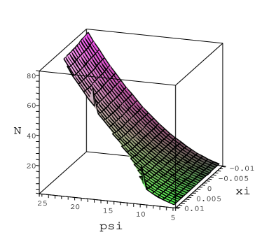
Figure 3: The number of e-folds for ranges of $\xi$ and $\psi_{0}$ for $V=m^{2}\phi^{2}/2$ (left panel) and for $V=\lambda\phi^{4}/4!$ (right panel).

An initial condition $\phi_{0}>m_{pl}$ is necessary for a sufficient inflation to occur in the large field model. The chaotic inflation belongs to this type. We consider $V=m^{2}\phi^{2}/2$ and $V=\lambda\phi^{4}/4!$ for the large field model. In Fig. 2, we compare the exact numerical solution and the slow-roll approximate solution of the Hamilton-Jacobi equation for $V=m^{2}\phi^{2}/2$ and $V=\lambda\phi^{4}/4!$. For $V=m^{2}\phi^{2}/2$, Eqs. (17) and (18) together with Eq. (9) become

$$W = \sqrt{\frac{4\pi G}{3}}\frac{m\phi}{1-8\pi G\xi\phi^{2}},$$ (21)

$$\frac{d\alpha}{d\phi} = -4\pi G\frac{\phi(1-8\pi G\xi\phi^{2}(1-6\xi))}{1-64\pi^{2}G^{2}\xi^{2}\phi^{4}}.$$ (22)

Integrating Eq. (22) over $\phi$ between $\phi_{0}$ and $\phi_{e}$, we can obtain the number of $e$-folds

$$\mathcal{N}=-\frac{1}{4\xi}({\rm arctanh}(\phi_{e}^{2}/\phi_{c}^{2})-{\rm arctanh}(\phi_{0}^{2}/\phi_{c}^{2}))-\frac{1-6\xi}{8\xi}\ln\frac{1-(\phi_{e}^{2}/\phi_{c})^{2}}{1-(\phi_{0}^{2}/\phi_{c}^{2})^{2}}.$$ (23)

After passing through the slow-roll regime, $\phi$ starts to oscillate around $\phi_{e}=0$. The number of $e$-folds are plotted in Fig. 3 (left) against $\psi_{0}\equiv\sqrt{8\pi}\phi_{0}/m_{pl}$ and $\xi$. In addition to the constraint from $G_{eff}>0$ for $\xi>0$, $\phi^{2}/\phi_{c}^{2}$ is further constrained by the form of ${\rm arctanh}$ function, independently of sign of $\xi$,

$$-1<\phi^{2}/\phi_{c}^{2}<1.$$ (24)

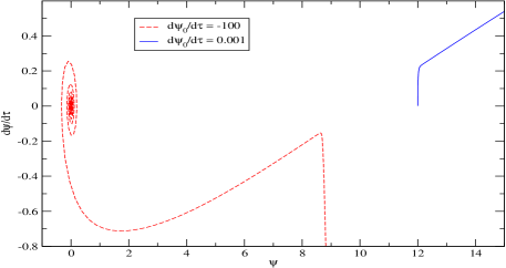
Figure 4: If $\xi$ is negative and $\phi_{0}>\phi_{m}$, the orbit of the scalar field depends on the initial value of $\dot{\phi}$ for $V=m^{2}\phi^{2}/2$. For $\xi=-10^{-2}$, $\psi_{0}\equiv\sqrt{8\pi G}\phi_{0}=12$, and $d\psi/d\tau=-100$, $\phi$ crosses over the peak of potential and evolves toward the origin. The origin is an attractor.

For $\xi<0$, the scalar field shows a different behavior depending upon the initial value $\phi_{0}$. If $\phi_{0}<\phi_{m}\equiv m_{pl}/\sqrt{8\pi|\xi|}=|\phi_{c}|$, the field $\phi$ evolves toward the origin. But if $\phi_{0}>\phi_{m}$, $\phi$ runs away to infinity and never reaches the origin. This constraint for $\xi<0$ is understood in the Einstein frame futamase89 ; tsujikawa00 . The potential in the Einstein frame can be obtained through a conformal transformation as

$$\hat{V}(\phi)=\frac{V(\phi)}{(1-\phi^{2}/\phi_{c}^{2})^{2}}.$$ (25)

The potential $\hat{V}$ has a local maximum at $\phi_{m}$ for $V=m^{2}\phi^{2}/2$ when $\xi$ is negative. If $\phi_{0}>\phi_{m}$, the field diverges to larger values as shown in Fig. 4 instead of rolling down to the origin. But if the initial value of $\dot{\phi}$ is very large and negative, the field crosses over the potential barrier and then reaches the origin. Even though it is possible for $\phi$ field to reach the origin when $\phi_{0}>\phi_{m}$ for $-10^{-3}<\xi<0$, the number of $e$-folds is not greater than $60$ because the slow-roll starts at $\phi\simeq\phi_{m}$. Thus, the initial condition $\phi_{0}$ should be less than $m_{pl}/\sqrt{8\pi|\xi|}$, independently of the sign of $\xi$. And a constraint $|\xi|\leq 10^{-3}$ is required for a sufficient inflation to occur. In this case, the first term in Eq. (23) dominates

$$\mathcal{N}\simeq\frac{1}{4\xi}{\rm arctanh}(\phi_{0}^{2}/\phi_{c}^{2}).$$ (26)

For $\mathcal{N}\gtrsim 60$, $\psi_{0}\equiv\sqrt{8\pi}\phi/m_{pl}\gtrsim 16.5$ when $\xi=10^{-3}$.

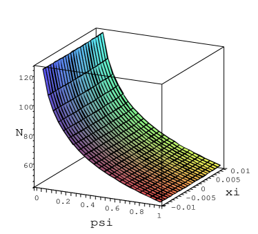
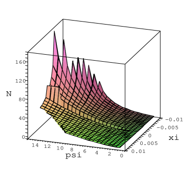
Figure 5: The number of e-folds for ranges of $\xi$ and initial values $\psi_{0}$ in the small field model (left panel) and in the hybrid model (right panel).

Next, we consider $V=\lambda\phi^{4}/4!$ and then Eqs. (17) and (18) become

$$W = \frac{\sqrt{\lambda\pi G}}{3}\frac{\phi^{2}}{1-8\pi G\xi\phi^{2}},$$ (27)

$$\frac{d\alpha}{d\phi} = -2\pi G\frac{\phi(1-8\pi G\xi\phi^{2}(1-6\xi))}{1-8\pi G\xi\phi^{2}}.$$ (28)

By simply integrating Eq. (28) we can get the number of $e$-folds

$$\mathcal{N}=-\frac{1-6\xi}{8\xi\phi_{c}^{2}}(\phi_{e}^{2}-\phi_{0}^{2})+\frac{3}{4}\ln\frac{1-\phi_{e}^{2}/\phi_{c}^{2}}{1-\phi_{0}^{2}/\phi_{c}^{2}}.$$ (29)

We plot the number of $e$-folds in Fig. 3 (right). For $\xi>0$, $\phi$ should be less than $\phi_{c}$ to satisfy the condition $G_{eff}>0$. A constraint $|\xi|<10^{-3}$ is also required in order to lead to a sufficient number of $e$-folds as for the case of $V=m^{2}\phi^{/}2$. A local maximum of the potential in the Einstein frame does not exist in this potential. Thus, there is no constraint on $\phi_{0}$ even when $\xi$ is negative. For $|\xi|<10^{-3}$, the first term in Eq. (29) dominates the second logarithmic term due to the factor of $(1-6\xi)/8\xi$. So for $|\xi|\leq 10^{-3}$ and $\phi_{e}\simeq 0$, we have initial conditions for $\mathcal{N}\geq 60$

$$\phi_{0}\geq\sqrt{\frac{60}{8\pi}}\sqrt{\frac{8}{1-6\xi}}m_{pl}.$$ (30)

III.2 A small field model, $V(\phi)\propto 1-(\phi/\mu)^{p}$

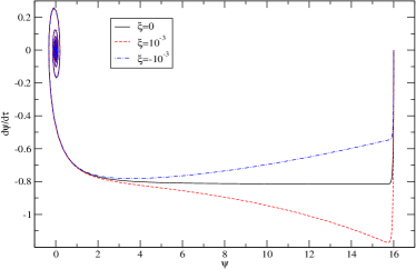
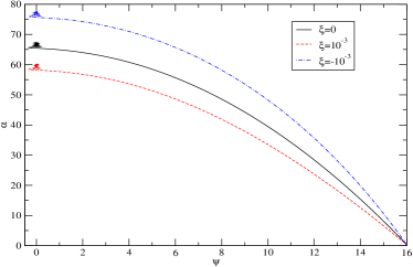
Figure 6: Phase diagram of $\psi\equiv\sqrt{8\pi G}\phi$ and $d\psi/d\tau$ (left panel) and $\alpha$ against $\psi$ (right panel) for $V(\phi)=m^{2}\phi^{2}/2$. An initial value $\psi_{0}=16$ is taken.

Let us consider a Ginzburg-Landau potential

$$V(\phi)=\frac{\chi}{8}(\phi^{2}-\mu^{2})^{2}.$$ (31)

If $|\phi|\gg\mu$, this potential can be regarded as a large field model with a term $\phi^{4}$ fakir90 . Therefore we assume that $|\phi|\ll\mu$. In the vicinity of the origin, this potential is approximated as

$$V(\phi)=\Lambda^{4}\left(1-\left(\frac{\phi}{\mu}\right)^{2}\right).$$ (32)

where $\Lambda=\mu(\chi/8)^{1/4}$. The field $\phi$ is initially located around the origin and then slowly rolls down to the true vacuum at $\mu=\langle\phi\rangle$. With the slow-roll condition, the Hamilton-Jacobi equation and the evolution equation for $\alpha$ become

$$W = \sqrt{\frac{\pi\chi G}{3}}\frac{\phi^{2}-\mu^{2}}{1-8\pi G\xi\phi^{2}},$$ (33)

$$\frac{d\alpha}{d\phi} = -\frac{2\pi G}{1-8\pi G\xi\mu^{2}}\frac{(\phi^{2}-\mu^{2})(1-8\pi G\xi\phi^{2}(1-6\xi))}{\phi(1-8\pi G\xi\phi^{2})}.$$ (34)

Then, the number of $e$-folds is

$$\mathcal{N}=\frac{1}{4(\phi_{c}^{2}-\mu^{2})}\Biggl{[}-\frac{1-6\xi}{2\xi}(\phi_{e}^{2}-\phi_{0}^{2})+\frac{\mu^{2}}{\xi}\ln\frac{\phi_{e}}{\phi_{0}}+3(\phi_{c}^{2}-\mu^{2})\ln\frac{1-\phi_{e}^{2}/\phi_{c}^{2}}{1-\phi_{0}^{2}/\phi_{c}^{2}}\Biggr{]}.$$ (35)

We assume that inflation ends when $\phi_{e}\simeq\mu$. In Eq. (35), if $1-\mu^{2}/\phi_{c}^{2}<0$, $\phi_{0}^{2}/\phi_{c}^{2}$ should be larger than $1$. However, this violates the condition $G_{eff}>0$ in Eq. (2) for $\xi>0$. So we restrict to $\mu^{2}/\phi_{c}^{2}<1$ for $\xi>0$. If $\phi\ll m_{pl}$, the second term in Eq. (35) dominates in the number of e-foldings

$$\mathcal{N}\simeq\frac{\mu^{2}}{4\xi(\phi_{c}^{2}-\mu^{2})}\ln\frac{\mu}{\phi_{0}}.$$ (36)

In Fig. 5 (left), we plot the number of $e$-foldings for various ranges of $\xi$ and $\psi\equiv\sqrt{8\pi G}\phi_{0}$ and $\sqrt{8\pi G}\mu=10$.

Note that the nonminimal coupling might prevent inflationary solutions in the new inflation abbott81 because the coupling term, $\xi R\phi^{2}/2$, behaves like a mass term in the scalar field potential and destroys the flatness of the potential near the origin. However, we will examine a possibility of the inflationary solutions in the new inflation when $\phi\ll\mu$ and $8\pi G\xi\phi^{2}\ll 1$. During the slow-roll of the inflation, the potential (31) can be approximated as $V\simeq\Lambda^{4}$. Then Eqs. (9) and (34) are approximated by

$$\dot{\phi} \simeq \sqrt{\frac{128\pi G\Lambda^{4}}{3}}\xi\phi,$$ (37)

$$\frac{d\alpha}{d\phi} \simeq \frac{2\pi G\mu^{2}}{1-8\pi G\xi\mu^{2}}\frac{1}{\phi}.$$ (38)

where we have set $N=1$. Thus we obtain the solutions

$$\phi=\phi_{i}\exp\left[\sqrt{\frac{128\pi G\Lambda^{4}}{3}}\xi t\right],\quad\alpha=\alpha_{i}\sqrt{\frac{8\pi G\Lambda^{4}}{3}}\frac{8\pi G\xi\mu^{2}}{1-8\pi G\xi\mu^{2}}t,$$ (39)

where $\phi_{i}$ and $\alpha_{i}$ are integration constants. Because $\alpha$ is a logarithm of the scale factor, this shows that the universe expands quasi-exponentially when the nonminimal coupling exists. But here we do not consider the dynamics of the phase transition in detail during the slow-roll phase, so it requires scrutiny to conclude about the existence of inflationary solutions in the new inflationary scenario.

III.3 A hybrid field model, $V\propto 1+(\phi/\mu)^{p}$

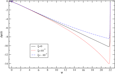
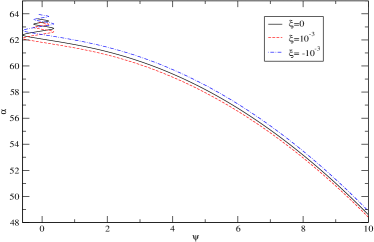
Figure 7: Phase diagram of $d\psi/d\tau$ and $\psi$ (left panel) and $\alpha$ against $\psi$ (right panel) for $V(\phi)=\lambda\phi^{4}/4!$. The initial value $\psi_{0}=22$ is taken.

This type of potential describes the hybrid inflation linde91 ; copeland94 . Contrary to the other inflation models, hybrid inflation gives a blue power spectrum. The potential in hybrid inflation may take the form

$$V(\sigma,\phi)=\frac{\lambda}{4}(M^{2}-\sigma^{2})^{2}+\frac{m^{2}}{2}\phi^{2}+\frac{g^{2}}{2}\phi^{2}\sigma^{2}.$$ (40)

When $\phi^{2}>\phi_{f}^{2}\equiv\lambda M^{2}/g$, there is a local minimum at $\sigma=0$ (false vacuum) on the constant $\phi$ slices. Inflation begins when $\sigma$ is located at the false vacuum ($\sigma=0$), and then the $\phi$ field rolls down toward the origin ($\phi=0$). During the inflation period and near $\sigma=0$, the potential can be given by

$$V(\phi)=\frac{\lambda}{4}M^{4}+\frac{1}{2}m^{2}\phi^{2}.$$ (41)

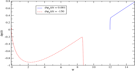
Figure 8: When $\xi<0$ and $\phi_{0}>\phi_{m}$, the orbit of the scalar field depends upon the initial value of $\dot{\phi}$ for $V=\Lambda^{4}(1+(\phi/\mu)^{2})$. For $\xi=-10^{-2}$, $\psi_{0}=12$, and $d\psi/d\tau=-150$, $\phi$ crosses over the peak of potential and evolves toward the origin as in the case of $V=m^{2}\phi^{2}/2$.

If the false vacuum energy dominates the potential energy, inflation ends when $\phi^{2}<\phi_{f}^{2}$. The hybrid field model differs from the large field model in the sense that during inflation the vacuum energy is nonzero. The potential, (41), can be rewritten as

$$V(\phi)=\Lambda^{4}\left(1+\left(\frac{\phi}{\mu}\right)^{2}\right),$$ (42)

where $\Lambda^{4}=\lambda M^{4}/4$ and $\mu^{2}=\lambda M^{4}/2m^{2}$. The Hamilton-Jacobi equation and the evolution equation for $\alpha$ become

$$W = \sqrt{\frac{8\pi G\Lambda^{4}}{3\mu^{2}}}\frac{\sqrt{\mu^{2}+\phi^{2}}}{1-8\pi G\xi\phi^{2}},$$ (43)

$$\frac{d\alpha}{d\phi} = -4\pi G\frac{(\mu^{2}+\phi^{2})(1-8\pi G\xi\phi^{2}(1-6\xi))}{\phi(1-8\pi G\xi\phi^{2})(1+16\pi G\xi\mu^{2}+8\pi G\xi\phi^{2})}.$$ (44)

By simply integrating Eq. (44), we obtain

$$\mathcal{N} = -\frac{1}{8\xi(1+2\mu^{2}/\phi_{c}^{2})}\Biggl{[}4\frac{\mu^{2}}{\phi_{c}^{2}}\ln\frac{\phi_{e}}{\phi_{0}}-6\xi\left(1+\frac{2\mu^{2}}{\phi_{c}^{2}}\right)\ln\frac{1-\phi_{e}^{2}/\phi_{c}^{2}}{1-\phi_{0}^{2}/\phi_{c}^{2}}$$ (45)

$$+\left(2-6\xi+\frac{2\mu^{2}}{\phi_{s}^{2}}\right)\ln\frac{1+2\mu^{2}/\phi_{c}^{2}+\phi_{e}^{2}/\phi_{c}^{2}}{1+2\mu^{2}/\phi_{c}^{2}+\phi_{0}^{2}/\phi_{c}^{2}}\Biggr{]}.$$

We assume that the inflaton field $\phi$ dominates the vacuum energy but the $\sigma$ field plays no significant role during the inflation period. This implies that $\mu\ll m_{pl}\ll\phi$ copeland94 . With this assumption, the third term in Eq. (45) is dominant compared to the other two terms. If we set $\phi_{e}\simeq 0$ and for $\xi<0$, note that the numerator in the second logarithmic term is greater than zero, then $8\pi G|\xi|\phi_{0}^{2}$ should be less than $1$. With the potential given in (41), this situation is similar to the large field model with $V=m^{2}\phi^{2}/2$. When $\xi$ is negative, the maximum value of the potential in the Einstein frame, (25), which could be obtained through the conformal transformation, is located at

$$\phi=\phi_{m}\equiv\frac{1-16\pi G|\xi|\mu^{2}}{8\pi G|\xi|}.$$ (46)

If $8\pi G|\xi|\mu^{2}\ll 1$, then $\phi_{m}\simeq m_{pl}/\sqrt{8\pi|\xi|}$. Similarly to the case of $V=m^{2}\phi^{2}/2$, even if the $\phi_{0}$ is greater than $\phi_{m}$, the $\phi$ field crosses over the barrier of the potential and then evolves toward the origin when it has a very large negative initial velocity. It is, however, required $\phi_{0}$ should be less than $\phi_{m}$ and $|\xi|\leq 10^{-3}$ as stated in the case of $V=m^{2}\phi^{2}/2$. The phase diagram for $\xi<0$ and $\phi_{0}>\phi_{m}$ are plotted in Fig 8. For $\mu\ll m_{pl}$, Eq. (45) could be approximated as

$$\mathcal{N}\simeq-\frac{2-6\xi}{8\xi}\ln\frac{1}{1+\phi_{0}^{2}/\phi_{c}^{2}}.$$ (47)

IV Numerical Solutions of Hamilton-Jacobi Equation

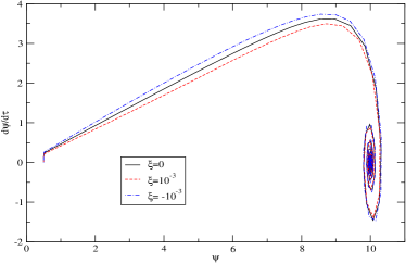
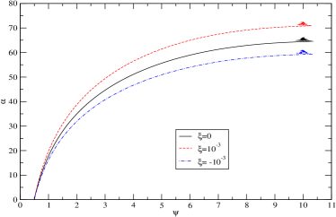
Figure 9: Phase diagram of $d\psi/d\tau$ and $\psi$ (left panel) and $\alpha$ against $\psi$ (right panel) for $V(\phi)=\chi(\phi^{2}-\mu^{2})^{2}/8$. We take the initial parameters $\psi_{0}=0.5$ and $\sqrt{8\pi G}\mu=10$.

In this section, we numerically solve the Hamilton-Jacobi equation (7) and the evolution equation (8) for $\alpha$ and Eq. (9) for $\phi$ in the nonminimally coupled scalar field theory. And then we compare this result with that of Einstein gravity, $\xi=0$ in this paper. $W$ could be interpreted as a Hubble parameter $H\equiv\dot{\alpha}/N$ for $\xi=0$. We choose the synchronous gauge ($N=1$) for numerical calculations and, using Eqs. (9) and (7), derive the second order differential equation for $\phi$

$$\ddot{\phi} = -3\sqrt{1-8\pi G\xi\phi^{2}}W\dot{\phi}-\frac{16\pi G\xi\phi}{1-8\pi G\xi\phi^{2}}\dot{\phi}^{2}\left[1-\frac{3\xi}{1-8\pi G\xi\phi^{2}(1-6\xi)}\right]$$ (48)

$$- \frac{1-8\pi G\xi\phi^{2}}{1-8\pi G\xi\phi^{2}(1-6\xi)}V_{,\phi}-\frac{32\pi G\xi\phi}{1-8\pi G\xi\phi^{2}(1-6\xi)}V.$$

The dimensionless quantities to be introduced are

$$\psi=\frac{\sqrt{8\pi}\phi}{m_{pl}},\quad\tau=\frac{t}{t_{\ast}},$$ (49)

where $t_{\ast}$ depends on the shape of the potential. We choose $t_{\ast}=1/m$ for $V=m^{2}\phi^{2}/2$, $t_{\ast}=\sqrt{8\pi/\lambda}/m_{pl}$ for $V=\lambda\phi^{4}/4!$, $t_{\ast}=\sqrt{8\pi/\chi}/m_{pl}$ for $V=\chi(\phi^{2}-\mu^{2})^{2}/8$, and $t_{\ast}=m_{pl}/\sqrt{8\pi}/\Lambda^{2}$ for $V=\Lambda^{4}(1+(\phi/\mu)^{2})$.

In Fig. 6, we plot the phase diagram and logarithm of the scale factor, $\alpha$, for $\phi$ for $V=m^{2}\phi^{2}/2$ when the initial value is prescribed by $\psi_{0}=16$. From the discussion in the previous section, $\psi_{0}^{2}$ should be smaller than $1/|\xi|$ for $V=m^{2}\phi^{2}/2$. Therefore, the constraint $|\xi|\lesssim 10^{-3}$ is required for a sufficient inflation to occur (see Fig. 3 (left)). Fig. 6 (left) shows an attractor at $(\phi,\dot{\phi})=(0,0)$ if the initial condition $\psi_{0}^{2}<1/|\xi|$ is satisfied. The number of $e$-folds in Fig. 6 (right) decreases for $\xi>0$ compared to the case of $\xi=0$ but is enhanced for $\xi<0$. As stated in the previous section, if $\psi$ is greater than $\psi_{m}=1/\sqrt{|\xi|}$ for $\xi<0$, the orbit in the phase diagram may reach the origin or evolve to larger values of $\psi$ depending on the velocity $d\psi/d\tau$. This is shown in Fig. 4. If $d\psi/d\tau=10^{-3}$ for $\xi=-10^{-2}$ and for $\psi_{0}=12$, which is larger than $\psi_{m}=10$, $\psi$ does not evolve toward the origin. On the contrary, if $d\psi/d\tau=-10^{2}$, it crosses over the peak of the potential and then reaches the attractor. However, if $|\xi|>10^{-3}$, it does not give a sufficiently enough inflation.

The phase diagram and number of $e$-folds for $V=\lambda\phi^{4}/4!$ are plotted in Fig. 7 with $\psi_{0}=22$. And $W$ against $\phi$ is plotted in Fig. 2 (right). For $\xi>0$, the initial value of $\psi$ is constrained by $\psi<1/\sqrt{\xi}$. So to have $\mathcal{N}\gtrsim 60$, one needs $\xi\lesssim 10^{-3}$. But, on the contrary to the case of $V=m^{2}\phi^{2}/2$, it is possible to have inflation for $\xi<0$, irrespective of the magnitude of $|\xi|$ (see Fig. 3 (right)). The attractor is shown at $(\phi,\dot{\phi})=(0,0)$ in Fig. 7 (left). As in the case of $V=m^{2}\phi^{2}/2$, $\mathcal{N}$ in Fig. 7 (right) decreases for positive $\xi$ compared to the $\xi=0$ case, whereas it increases for negative $\xi$. The number of $e$-folds, however, do not much depend on $\xi$. The initial condition $\psi_{0}>22$ is at least needed for $\xi=10^{-3}$ in Eq. (30).

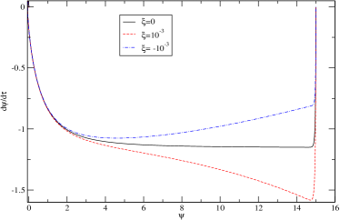
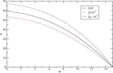
Figure 10: Phase diagram of $d\psi/d\tau$ and $\psi$ (left panel) and $\alpha$ against $\psi$ (right panel) for $V(\phi)=\Lambda^{4}(1+(\phi/\mu)^{2})$. We take the initial parameters as $\psi_{0}=15$ and $\sqrt{8\pi G}\mu=1$.

In Fig. 9, the phase space diagram and number of $e$-folds are plotted for the small field model with the potential (31). Contrary to the large field model, the attractor in phase diagram is located at $(\phi,\dot{\phi})=(\mu,0)$, where $\mu=\langle\phi\rangle$. We have chosen $\psi_{0}=0.5$ and $\sqrt{8\pi G}\mu=10$. Inflationary solutions are shown in Fig. 9 (right), which can be seen from $\alpha\propto\ln\phi$ implying a quasi-exponential expansion of the scale factor. The field is initially located at the origin ($\psi_{0}\ll 1$) and then evolves to the minimum of the potential, $\mu$. When the field arrives at the minimum, the inflation ends and the field starts to oscillate around the minimum. As long as $\psi_{0}\ll 1$, there is no constraint on the $\psi_{0}$ (see Fig. 5 (left)) but for $\xi>0$, $\mu$ must be less than $1/\sqrt{8\pi G\xi}$. The number of $e$-folds, $\mathcal{N}$, increases for $\xi>0$ relative to the $\xi=0$ case, which differs from the case of the large field model, but it decreases for $\xi<0$.

We plot the phase diagram and number of $e$-folds in Fig. 10 for the hybrid inflation potential. We put the parameters $\psi_{0}=15$ and $\sqrt{8\pi G}\mu=1$. Starting from $\psi_{0}$, the field rolls down toward the false vacuum, $V=\Lambda^{4}$. Similarly to the large field model with $V=m^{2}\phi^{2}/2$, the hybrid inflation also gives the constraint on $\psi_{0}$ as $\psi_{0}^{2}<1/|\xi|$. This constraint comes from the condition $G_{eff}>0$ for $\xi>0$ and the potential barrier of hybrid inflation in the Einstein frame which prevents the field from reaching the origin for $\xi<0$. In Fig. 5 (right), $\mathcal{N}$ is plotted for possible $\psi_{0}$ and $\xi$. It shows that a constraint of $|\xi|\leq 10^{-3}$ is needed for $\mathcal{N}\gtrsim 60$. Similar arguments in the case of $V=m^{2}\phi^{2}/2$ are possible for $\xi<0$ when the field initially is located in the region larger than the peak of the potential, $\psi_{m}=1/|\xi|$. If the initial velocity ($d\psi/d\tau$) of the field is much small, the field evolves to larger values of $\psi$ and does never arrive at the origin. But if the field has a large and negative initial velocity, then the field crosses over the peak of the potential and then evolves to the origin. We plot the phase diagram for $\xi<0$ when the $\psi>\psi_{m}=10$ in Fig. 8. We compare $d\psi/d\tau=0.001$ with $-150$ for $\xi=-10^{-2}$.

V summary

Using the Hamilton-Jacobi theory we have studied nonlinear evolutions of inhomogeneous spacetimes when scalar fields are nonminimally coupled with the spacetime curvature $R$. And we have found analytic and numerical solutions for several classes of inflation potentials during the inflation period. The inflation potentials thus studied could be categorized into three different types - a large field, small field, and hybrid field model, depending on the potential shape and the initial condition of scalar fields. Though it is believed that in the nonminimally coupled scalar theory, the new inflation, a small field model, may not have an inflationary solution, we have shown through an approximation and numerics that the new inflation potential can provide a quasi-exponential inflationary solution. Careful scrutiny is in order before reaching a definite conclusion for the existence of inflationary solutions. For the hybrid inflation potential, we have assumed that the inflaton field dominates the potential. However, if the potential is dominated by the vacuum energy, which is the limit of the small field model, the other scalar field, $\sigma$, plays a significant role in terminating the inflation. It would be interesting to consider the inflationary solutions for multi-field potentials.

In the case of $\xi>0$, the coupling constant is restricted to a range of $\xi<10^{-3}$ to have the number of $e$-folds greater than $60$ whose value is needed to resolve the well known cosmological puzzles. On the other hand, in the case of $\xi<0$, $V=\lambda\phi^{4}/4!$ in the large field or small field model does not lead to any constraint on $\xi$ to satisfy the observational bound on $\mathcal{N}$, but $V=m^{2}\phi^{2}/2$ in the large field model or hybrid field model with $\mu\ll\phi$, the scaled field $\psi_{0}\equiv\sqrt{8\pi}\phi_{0}/m_{pl}$ should be smaller than $1/|\xi|$ and $|\xi|<10^{-3}$. If these potentials in the original frame called Jordan frame are transformed into those in the Einstein frame by a conformal transformation, the local maxima of the potentials are located at $\phi_{m}=1/\sqrt{8\pi G|\xi|}$ for $V=m^{2}\phi^{/}2$ and $\phi_{m}=(1-16\pi G|\xi|\mu^{2})/8\pi G|\xi|$ for the hybrid field model. If the field $\phi$ is greater than $\phi_{m}$, it goes away to infinity and never reaches the origin. However, if the scalar field has a very large negative initial velocity, it can cross over the potential barrier and evolve toward the origin. But the number of $e$-folds being greater than $60$ restricts to the nonminimal coupling constant to $|\xi|<10^{-3}$.

It would be more helpful to understand analytically or numerically the behaviors of nonlinear evolutions of inhomogeneous spacetimes in the nonminimally coupled scalar field theory beyond the zeroth order Hamilton-Jacobi equation, which will be addressed in a future publication.

References

(1) J. Maldacena, J. High Energy Phys. 05, 013 (2003);
N. Bartolo, E. Komatsu, S. Matarrese, and A. Riotto, Phys. Rep. 402,
103 (2004).
(2) D. S. Salopek and J. R. Bond, Phys. Rev. D 42,
3936 (1990).
(3) S. Koh, S. P. Kim, and D. J. Song, astro-ph/0501401
(4) J. Soda, H. Ishihara, and O. Iguchi, Prog. Theor. Phys.
94, 781 (1995).
(5) J. E. Lidsey et al., Rev. Mod. Phys. 69,
373 (1997).
(6) S. Dodelson, W. H. Kinney, and E. W. Kolb, Phys. Rev. D
56, 3207 (1997); W. H. Kinney, ibid.58, 123506 (1998).
(7) A. D. Linde, Phys. Lett. B 129, 177 (1983).
(8) A. D. Linde, Phys. Lett. B 108, 389 (1982);
A. Albrecht and P. J. Steinhardt, Phys. Rev. Lett. 48, 1220 (1982).
(9) A. Linde, Phys. Lett., B 259,38 (1991); A. D. Linde,
Phys. Rev. D 49, 748 (1994).
(10) E. J. Copeland, A. R. Liddle, D. H. Lyth,
E. D. Stewart, and D. Wands, Phys. Rev. D 49, 6410 (1994).
(11) T. Futamase and K. Maeda, Phys. Rev. D 39,
399 (1989).
(12) R. Fakir and W. G. Unruh, Phys. Rev. D 41, 1783 (1990).
(13) S. Tsujikawa, Phys. Rev. D 62, 043512 (2000);
S. Tsujikawa and B. Gumjudpai, Phys. Rev. D 69,
123523 (2004).
(14) L. F. Abbott, Nucl. Phys. B 185, 233 (1981);
V. Faraoni, Phys. Rev. D 53, 6813 (1996).