Abstract

We present a review of the history and the present state of the fractal approach to the large-scale distribution of galaxies. The roots of the modern idea of cosmic fractality go to the beginning of the 20th century, when hierarchical world models were proposed by Fournier and Charlier. Fundamental aspects of hierarchical matter distribution was discussed by Einstein and Selety in the correspondence concerning inhomogeneous cosmological models.

The Great Debate on the nature of spiral nebulae went over to a struggle on the structure and extension of the galaxy clustering. Already during the epoch of galaxy angular catalogues astronomers detected superclusters of galaxies on the sky. However, early counts of bright galaxies were close to the $0.6m$-law, pointing to homogeneity. Also the debated variable extinction seemed to be a reasonable explanation of apparent galaxy clustering. Angular correlation function analysis gave small a homogeneity scale $R_{\mathrm{hom}}\approx 10$ Mpc within which the correlation exponent corresponds to a fractal dimension $D\approx 1.2$ and outside which the galaxy distribution is homogeneous.

It was realized later that a normalization condition for the reduced correlation function estimator results in distorted values for both $R_{\mathrm{hom}}$ and $D$. Moreover, according to a theorem on projections of fractals, galaxy angular catalogues can not be used for detecting a structure with the fractal dimension $D\geq 2$. For this 3-d maps are required, and indeed modern extensive redshift-based 3-d maps have revealed the “hidden” fractal dimension of about 2, and have confirmed superclustering at scales even up to 500 Mpc (the Sloan Great Wall). On scales, where the fractal analysis is possible in completely embedded spheres, a power–law density field has been found.

Two new fundamental cosmic numbers have appeared, the fractal dimension $D$ and the crossover scale to homogeneity $R_{\mathrm{hom}}$. Their values have been debated, and $D=1.2$ indirectly deduced from angular catalogues has been replaced by $D=2.2\pm 0.2$ directly obtained from 3-d maps and $R_{\mathrm{hom}}$ has expanded from 10 Mpc to scales approaching 100 Mpc. In concordance with the 3-d map results, modern all sky galaxy counts in the interval $10^{m}\div 15^{m}$ give a $0.44m$-law which corresponds to $D=2.2$ within a radius of 100$h^{-1}_{100}$ Mpc. The narrow cones of the existing deep galaxy surveys and poorly known peculiar velocities at small scales are still the main limiting factors hampering precise estimates of $D$ and $R_{\mathrm{hom}}$. We emphasize that the fractal mass–radius law of galaxy clustering has become a key phenomenon in observational cosmology. It creates novel challenges for theoretical understanding of the origin and evolution of the galaxy distribution, including the role of dark matter and dark energy.

CONTENTS

1. Introduction

2. The fractal view of large-scale structure of the Universe

2.1.The idea of a self-similar universe

Protofractals

Fournier d’Albe and Carl Charlier

2.2.Genuine fractal structures

Self-similarity and power law

Fractal dimension

2.3. Concepts of density field

Ordinary fluid-like density fields

Ordinary stochastic discrete processes

Fractal density fields

2.4.Exclusive properties of fractals

Power-law density-radius relation

Massive, zero-density universes

Lower and upper cutoffs

Lacunarity

Projection and intersection

Multifractal structures

2.5.Modern redshift and photometric distance surveys

Redshift surveys

Limits of a survey

Galaxy catalogues based on photometric distances

How to discover fractal structure?

3. Statistical methods to detect fractal structures

3.1.Definitions for correlation functions

Complete and reduced correlation functions

Mass variance in spheres and characteristic scales

3.2.The method of $\xi$ correlation function

Peebles’ $\xi$ correlation function

$\xi$-function estimators

The normalization condition for $\xi$ estimators

A systematic distortion of the true power-law

Redshift space and peculiar velocity field

3.3.The method of conditional density $\Gamma$

Definitions

$\Gamma$-function estimator

$\Gamma(s)$ and peculiar velocities

$\Gamma$-function for intersections

3.4.Comparision of $\xi$ and $\Gamma$ analyses

The relation between $\Gamma$ and $\xi$

Power-law correlation and fractal density field

Dependence of $r_{0}$ on the sample parameters

Geometry and characteristic scales of a survey

3.5.Nearest neighbours distribution

Poisson distribution

Fractal distribution

3.6.Two-point conditional column density

Definitions

Estimation

3.7.Fourier analysis of the structures

Ordinary density field

Fractal density field

Geometry of surveys

3.8.Multifractals and luminosity function

Spectrum of fractal dimensions

Schechter’s luminosity function

Space-luminosity correlation in multifractal model

4. The epoch of galaxy angular position catalogues

4.1.The birth of the debate

Einstein–Selety correspondence

Retrospective view on the posed questions

4.2.Early arguments for galaxy clustering

Observations disclose clusters of galaxies

Santa Barbara 1961 conference

The cosmological de Vaucouleurs law

4.3.Early arguments for homogeneity

Hubble’s counts of bright galaxies

Hubble’s deep galaxy counts

Variable dust extinction

The classical “linearity” argument

Isotropy in a homogeneous universe

4.4.Results from angular catalogues

Main catalogues of galaxies and clusters

The angular correlation function analysis

Angular and spatial correlation functions

Hierarchical $D=1.2$ models

Tallinn 1977 conference

First evidence for $D=2$ galaxy distribution

Why did angular catalogues lose information about the $D=2$ structures?

5. Debate on fractality: the epoch of spatial maps

5.1.The fractal breakthrough in the 1980s.

Davis & Peebles $\xi$ correlation function analysis of the CfA sample of galaxies

The puzzling behaviour of the $\xi$-function

Pietronero’s solution the mystery of $r_{0}$

Balatonfurd 1987 conference

Multifractal controversy for $D_{2}=1.2$ estimation

The size of a fractal cell in the Universe

5.2.Further steps in the debate

Princeton “Dialogues’96”: Davis’s evidence for homogeneity

Princeton “Dialogues’96”: Pietronero’s arguments for fractality

The problem of sky projection of fractals

Modern research topics on fractality

5.3.Recent results from the $\xi$ and $\Gamma$ functions analyses

The redshift space $\xi$- and $\Gamma$- functions

The problem of peculiar velocity field

Dependence of $r_{0}$ on sample parameters

Power spectrum and intersection of fractals

5.4.Other results of the fractal approach

The two-point conditional column density

Number counts of all-sky bright LEDA galaxies

Radial counts of KLUN galaxy sample

6. Why fractality is important for cosmology

6.1.Basic elements of cosmological models

Three major empirical laws in cosmology

Theoretical basis of modern cosmology

The standard cosmological model

Fractal sources for gravity field

6.2.The origin and evolution of large scale fractals: challenges for theoretical models

Hubble law within fractal galaxy distribution

Problem of the origin of the fractal structure

6.3.The Cosmological Principle

Einstein’s cosmological principle

Derivation of homogeneity from isotropy

Mandelbrot’s cosmological principle

Towards Einstein-Mandelbrot concordance

7. Concluding remarks

References

1 Introduction

In this review we discuss the historical roots, methodological problems and modern results that branch of observational cosmology, which has given rise to the “Great Debate on Fractality”. This sharp and sometimes dramatic debate has been in the limelight almost the whole 20th century and still is. It has involved such persons as Einstein, Hubble, Sandage, Peebles, Charlier, Selety, Lundmark, de Vaucouleurs, Mandelbrot, Pietronero and many others who appear in the story.

The debate on the fractality of the large scale galaxy distribution has been going on around two new fundamental empirical cosmic numbers, — the fractal dimension $D$ and the bordering scale where fractality transforms into homogeneity $R_{\mathrm{hom}}$. The discussion of galaxy clustering started from scales $1\div 10$ Mpc, then observations of the large scale structure (LSS) have shifted to the scales of $10\div 100$ Mpc, and now we are entering gigantic scales of $100\div 1000$ Mpc.

There are several recent papers and books devoted to the LSS analysis, which are close to the subject of our review (Sylos Labini et al. 1998; Martinez & Saar 2002; Gabrielli et al. 2004; Jones et al. 2004). However, what has been lacking is a picture of historical steps in the studies of the large scale structure with a focus on methodological problems and challenges of current research. Our review addresses these questions.

A fundamental task of practical cosmology is to study how matter is distributed in space and how it has evolved in cosmic time. The discovery of the strongly inhomogeneous spatial distribution of galaxies, at scales from galaxies to superclusters, i.e. over four orders of magnitude in scale, was of profound cosmological significance. Only faintly anticipated from photographic surveys, the surprisingly rich texture of galaxies became visible thanks to a large progress in measuring distances by redshifts for thousands of galaxies. The observed clustering is not just random clumping, but obeys a universal law. The two major theoretical tools, the correlation function and the conditional density analyses, both have revealed a power law dependence of the galaxy number density on the length scale, on scales $0.1\div 10$ Mpc. This signature of the scale invariance or fractality of the galaxy distribution has opened a new application of fractal geometry, widely used in modern statistical physics.

In this review we present the growing evidence for fractality of the large scale galaxy clustering. In sect.2 we give a brief introduction to the concept of fractal density field. In sect.3 basic statistical methods for analysis of galaxy distribution are described. Sect.4 is devoted to the main arguments for and against galaxy clustering, debated during the epoch of angular galaxy catalogues. Such 2-d data do not contain information on distance, and what is even more important, they are not sensitive to a distribution with the fractal dimension $D\geq 2$. In sect.5 we summarize results obtained in the modern 3-d epoch from extensive redshift surveys which have revealed the “hidden” fractal dimension of about two, and have detected structures at scales up to 500 Mpc. One has seen how the value of $D=1.2$ derived from the angular catalogues has been replaced by $D=2.2\pm 0.2$ in 3-d maps and the maximum observed scale of fractality $R_{hom}$ has increased from 10 Mpc to scales approaching 100 Mpc. In sect.6 we consider cosmological importance of the observed large scale fractality.

2 The fractal view of the large scale structure of the Universe

The last two decades have seen the first extensive surveys of galaxy redshifts, which have permitted us to move from the study of the angular distribution of galaxies on the celestial sphere to the analysis of their three-dimensional distribution in space.

Already the first redshift surveys revealed a rich variety of structures in the galaxy universe. These have been characterized by astronomers using terms such as binaries, triplets, groups, rich, regular, and irregular clusters, walls, superclusters, voids, filaments, cells, soap bubbles, sponges, great attractors, clumps, concentrations, associations …Of course each form of structure deserves separate studies, but they can be also viewed as natural appearances of one global master entity which is called a fractal. By using this self-similar structure one can describe an inhomogeneous galaxy distribution by means of one basic parameter, the fractal dimension $D$, which determines the global mass–radius behaviour of the Universe.

However, it took a lot of time to recognize in the clumpy galaxy distribution on the celestial vault the signature of fractal structures. It is interesting and useful to see how the idea of self-similarity emerged in ancient times and developed into first protofractal models.

2.1 The idea of a self-similar universe

2.1.1 Protofractals

The ancestors of fractals appeared in old cosmological thinking. In the presocratic Greece the philosopher Anaxagoras of Clazomenae (about 500 - 428 B.C.), who spent a large part of his life teaching at Athens, put forward his theory of seeds. Only fragments of his text have been preserved, but these give the impression that the theory was based on ideas reminiscent of self-similarity (e.g. Grujić 2001, 2002). Contrary to atomists, he regarded the matter divisible without a limit, and his famous words are: “In all things there is a portion of everything.”

What has been called by Mandelbrot a protofractal, appeared as simple hierarchies in the 18th century works by Swedenborg, Kant and Lambert. Emanuel Swedenborg (1688–1772) was a Swedish scientist and visionary who was appointed, at the age of 28, assessor extraordinar in the Swedish College of Mines. A very productive thinker and writer, he discussed practically all fields of science of his time. In 1734, in his Principia, Swedenborg put forward the remarkable view of self- similarity and cosmic hierarchy, which was related to his general opinion that everything in the world is constructed according to a common plan.

The next steps were made by Immanuel Kant (1724-1804) and Johann Lambert (1728-1777) with their hierarchic systems. For example, Kant wrote in his book available in translation as Kant (1755): We see the first members of a progressive relationship of worlds and systems; and the first part of this infinite progression enables us already to recognize what must be conjectured of the whole. There is no end but an abyss $\cdots$ without bound.

But there was an essential difference between these world models. Kant, and perhaps Swedenborg, imagined that the hierarchy continues without end towards larger levels of celestial systems: it was an infinite hierarchy. Lambert thought that after a large (he cites the figure 1000 as an example), but finite number of steps, the hierarchy ends. He thought that the stellar systems are kept together by the gravity of a dark mass: … in the end you arrive at the middle point of the whole world structure and there I find my ultimate mass which governs the whole creation.

John Herschel (1792–1871) was, among many others, intrigued by the dark sky or Olbers’s Paradox (Harrison 1987). And he outlined a solution in a private letter: $\ldots$ it is easy to imagine a constitution of a universe literally infinite which would allow of any amount of such directions of penetration as not to encounter a star. Granting that it consists of systems subdivided according to the law that every higher order of bodies in it should be immensely more distant from the centre than those of the next inferior order - this would happen.

Herschel had in mind some kind of a hierarchical system. In another text he gives as examples the satellites of the planets of the solar system and the large distances between stars and asserts that “the principle of subordinate grouping” assumes “the character and importance of a cosmical law”.

2.1.2 Fournier d’Albe and Carl Charlier

The idea of a hierarchic structure of the universe was blown into life again by Edmund Fournier d’Albe (1868–1933). In 1907 he published the remarkable book Two new worlds where one finds a mathematical description of a possible hierarchical distribution of stars. In Fournier’s world (Fig.1) the stars are distributed in a hierarchy of spherical clusters in an infinite space, so that the mass inside each sphere increases directly proportionally to its radius:

$$M(R)\propto R\,.$$ (1)

Of course, this makes it dramatically different from the mass–radius behaviour in a homogeneous universe where $M(R)\propto R^{3}$. This was Fournier’s idea of how to avoid cosmological paradoxes appearing in Newton’s universe.

The cosmic hierarchy was further studied by the Swedish astronomer Carl Charlier (1908) in his article How an infinite world may be built up. After enthusiastic inspection of Fournier’s book, he developed more general models of stellar distributions which also solve the Olbers’s paradox and the riddle of infinite gravitational potential.

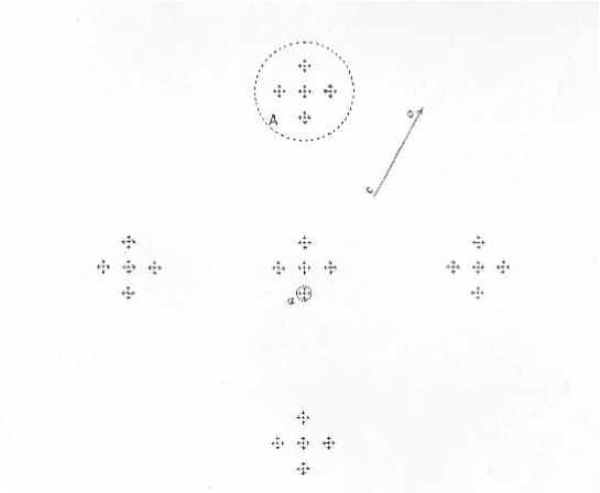
Figure 1: Fournier’s (1907) regular hierarchic world model. The same elements are repeated on different levels in a self–similar way. The average density $\rho(R)$ within the scale $R$ decreases with increasing scale $R$, hence $\rho(R)\rightarrow 0$ for $R\rightarrow\infty$.

Charlier found a criterion which the hierarchy must fulfil so that it will solve the mentioned paradoxes. The decisive factor is how fast the density decreases from one level (i) to the next one (i+1), and this depends on the ratio of the sizes of the successive elements and on the number $N_{i+1}$ of the lower elements forming the upper element. Denoting the sizes (radia) with $R_{i}$ and $R_{i+1}$, Charlier’s first criterion may be written as

$$R_{i+1}/R_{i}\geq N_{i+1}$$ (2)

or the size of upper level element divided by size of lower level element is larger or equal to the number of lower elements forming the upper elements. For example, Fournier’s illustration fulfils Charlier’s first criterion: there $N_{i}=N_{i+1}=5$, and the size ratio is always about 7.

In Charlier (1922), after a note by Selety (1922), a second criterion was derived:

$$R_{i+1}/R_{i}\geq\sqrt{N_{i+1}}$$ (3)

In terms of a continuous mass–radius behaviour for identical particles with mass $m$ the first criterion corresponds to $M(R)=mN(R)\propto R^{1}$. The second criterion, $M(R)\propto R^{2}$, and it is sufficient to cope with Olbers’ paradox and the infinite gravity force. The original Fournier’s (and the first Charlier’s) criterion is a stronger condition, and allows also a finite gravitational potential and finite stellar velocities.

2.2 Genuine fractal structures

Even though Fournier’s and Charlier’s hierarchies were overly simple for the real world, as we now know, they contained the seeds of the modern concept of genuine fractal. Regular hierarchical models (like in Fig.1) have a number of preferred scales, corresponding to the sizes of clusters at the level “$i$”. A great advantage of stochastic fractals is that they can be used to model scale-invariant galaxy clustering without preferred scales (Fig.2).

Though fractal geometry emerged just a few decades ago, some elements of it can be found already in the works of Poincaré and Hausdorff about a century ago. Mandelbrot (1975) introduced the name ”Fractals” and gave the following definition: A fractal is a set for which the Hausdorff dimension strictly exceeds the topological dimension.

Mandelbrot realized that fractal geometry is a powerful tool to characterize intrinsically irregular system. Nature is full of strongly irregular structures; trees, clouds, mountains and lightnings are familiar objects, which have in common the property that if one magnifies a small portion of them, a complexity comparable to that of the entire structure is revealed. This is geometric self-similarity.

Fractals are simple but subtle, as Luciano Pietronero likes to say, and becoming familiar with them requires some training of intuition. Here we briefly describe the essential properties of fractals, which are used in studies of the galaxy distribution. We recommend Mandelbrot (1982) for an original presentation by the father of fractals and Falconer (1990) for a special mathematical treatment. Here we emphasize observational consequences of self-similarity so that if this important property is actually present in galaxy data, one will be able to detect it correctly.

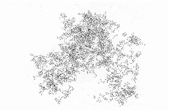
Figure 2: An example of a genuine stochastic fractal structure with the fractal dimension $D=1.26$ in two-dimensional space (B. Mandelbrot 1989).

2.2.1 Self-similarity and power law.

The difference between a self-similar distribution and a distribution with an intrinsic characteristic scale was clearly discussed by Coleman & Pietronero (1992). From a mathematical point of view self-similarity implies that the rescaling of the length $r$ by a factor $\>b$

$$r\rightarrow r^{\prime}=br$$ (4)

leaves the considered property, presented by an arbitrary function $f(r)$, unchanged apart from a renormalization that depends on $\>b$ but not on the variable $\>r$. This leads to the functional relation

$$f(r^{\prime})=f(b\cdot r)=A(b)\cdot f(r)$$ (5)

This is satisfied by a power law with any exponent. In fact for

$$f(r)=f_{0}r^{\alpha}$$ (6)

we have

$$f(r^{\prime})=f_{0}(br)^{\alpha}=(b)^{\alpha}f(r).$$ (7)

Here the exponent $\alpha$ defines the behaviour of the function everywhere. There is no preferred scale. It is true that the condition on the amplitude $\>f(r_{0})=1$ implies a certain length $r_{0}$

$$r_{0}=f_{0}^{-1/\alpha},$$ (8)

and one might be tempted to call $r_{0}$ a characteristic length, but this is quite misleading for self-similar structures! The power law refers to a fractal structure that was at the beginning constructed as self-similar and therefore cannot posses a characteristic length.

In eq.8 the value of $\>r_{0}$ is just related to the amplitude of the power law, and the amplitude has nothing to do with the scaling property. Instead of the value 1 for the amplitude, one could have used any other number in the relation $\>f(r_{0})=1$ to obtain other lengths. This is a subtle point of self-similarity; there is no reference value (like the average density) with respect to which one can define what is big or small.

This behaviour of the power-law is in contrast with the case of the exponential decay function where there is an intrinsic characteristic parameter $r_{0}$

$$g(r)=g_{0}e^{-r/r_{0}}$$ (9)

which determines a preferred length scale for the behaviour of the function. In the power-law the constant, dimensionless exponent $\alpha$ is not related to length scales at all.

2.2.2 Fractal dimension

The basic characteristics of a fractal structure is its dimension. The fractal dimension is a measure of the “strength of singularity” around the structure points. If there is a zero-level of structure elements, as in physical fractals where there is no mathematical singularity, the rate of growth of density with a decreasing spatial scale still defines the fractal dimension.

Let us consider the simplest example of a regular fractal structure to illustrate how the fractal dimension can be determined. Starting from a point occupied by an object we count how many objects are present within a sphere of radius $r$ in order to establish a number-radius relation from which one can define the fractal dimension $D$. Suppose that in the structure of Fig.1 we can find $N_{0}$ objects with mass $m_{0}$ in a volume of size $\>r_{0}$. If we consider a larger volume of size $\>r_{1}=k_{r}\cdot r_{0}$ we will find $\>N_{1}=k_{N}\cdot N_{0}$ objects. In a self-similar structure the parameters $\>k_{r}$ and $\>k_{N}$ will be the same also for other changes of scale. So, in general in a structure of size $\>r_{n}=k^{n}_{r}\cdot r_{0}$ we will have $\>N_{n}=k^{n}_{N}\cdot N_{0}$ objects. We can then write the relation between the number $\>N$ (or mass $M=m_{0}N$) and length $\>r$ in the form

$$N(r)=B\cdot r^{D}\,,\,\,\,\,\mathrm{or}\,\,\,\,M(r)=m_{0}B\cdot r^{D}$$ (10)

where the fractal dimension is the exponent $D$ of the power law, i.e.

$$D=\frac{\log{k_{N}}}{\log{k_{r}}}$$ (11)

depends on the rescaling factors $\>k_{r}$ and $\>k_{N}$. The prefactor $\>B$ is related to the zero-level parameters $\>N_{0}$ and $\>r_{0}$,

$$B=\frac{N_{0}}{r_{0}^{D}}\,.$$ (12)

We note that Eq.10 corresponds to a smooth continuous presentation of a strongly fluctuating function as is evident from Fig.1. The smooth average power-law for a fractal structure is always accompanied by large fluctuations and clustering at all scales.

Simple algorithms for constructing stochastic fractal structures with given fractal dimension one may find e.g. in Gabrielli et al. (2004). With these algorithms one may build artificial galaxy catalogues useful for testing different methods of structure analysis.

2.3 Concepts of density field

The definition of density field is the basis of the large scale structure analysis. There is an essential conceptual difference between ordinary and fractal density fields. The former kind of model is usually utilized for the description of gas or fluid dynamics having short range of correlations, while the latter one emerges in physical systems with strong long range scale-invariant fluctuations.

2.3.1 Ordinary fluid-like density fields

The concept of the density of a continuous medium (approximating fluid or gas), as it is normally used in hydrodynamics, contains the assumption that there exists a value of density independently of the size of the volume element $dV$. Then one may define the density $\rho(\vec{x})$ at a point $\vec{x}$ and regard it as a usual continuous function of position in space:

$$\rho_{{}_{fluid}}=\rho(\vec{x})=\lim_{V\rightarrow 0}\frac{M(\vec{x},V)}{V}$$ (13)

where $M$ is the mass of the fluid inside the volume $V$ around the point $\vec{x}$. For ordinary continuous media the limit exists and does not depend on the volume $V$, because at sufficiently small scales homogeneity is reached, i.e. $M=\rho V$.

When one studies fluctuations of an ordinary fluid, one can regard $\varrho(\vec{x})$ as one realization of a stochastic process for which the usual statistical moments are defined – average, dispersion etc.

Models for ordinary density fields go under the common name fluid-like correlated distributions. These have a uniform average background with superimposed fluctuations that are correlated. An example of such a fluctuation may be seen in Fig.3, top. Main properties of such distributions, in comparison with fractal distributions, are discussed by Gabrielli et al. (2004).

An ordinary stationary stochastic density field $\rho(\vec{x})$ may be represented as a sum of density fluctuations $\delta\rho(\vec{x})$ and the mean constant density $\rho_{0}=\langle\rho(\vec{x})\rangle$, so that

$$\rho(\vec{x})=\rho_{0}+\delta\rho\,,$$ (14)

or in terms of the dimensionless relative density fluctuation:

$$\delta(\vec{x})=\frac{\rho-\rho_{0}}{\rho_{0}}=\frac{\delta\rho(\vec{x})}{\rho_{0}}\,.$$ (15)

Note that the relative fluctuation $\delta(x)$ in Eq.15 has positive and negative values in the range $-1\leq\delta(x)<\infty$, while the density field is always positive $\rho(x)>0$ for positive masses of particles.

One usually considers $\delta\rho(\vec{x})$ as a realization of a Gaussian stochastic process, for which the phases of fluctuations are uncorrelated. Here a fundamental role is played by the average density $\bar{\rho}=$ const $>0$ which should exist and be well defined and positive for each realization of the random process $\rho(x)$. “Well defined” means that the average density does not depend on the size and location of a fair test volume.

2.3.2 Ordinary stochastic discrete processes

Ordinary density field may be also presented by a discrete stochastic process, called a stochastic point process or a point-particle distribution. Here discreteness introduces some new aspects related to point-like singularity of particles.

An important example of a homogeneous stochastic discrete density field is the Poisson process, giving rise to a number density of particles $n(\vec{x})=\Sigma_{i=1}^{N}\delta(\vec{x}-\vec{x}_{i})$. According to the Poisson law the probability $P$ to find $N$ particles in a volume $V$ is

$$P(N,V)=\frac{\langle N\rangle^{N}\exp(-\langle N\rangle)}{N\mathrm{!}}\,,$$ (16)

where $\langle N\rangle=n_{0}V$ is the average number of particles in the volume $V(r)$. The only parameter of the Poisson distribution is the constant number density $n_{0}=\langle n(\vec{x})\rangle$, or intensity of the Poisson process. It determines a characteristic scale $\lambda_{0}$ for this process

$$\lambda_{0}\approx n_{0}^{-1/3}\approx R_{sep}\,\,,$$ (17)

which is about the average distance between the particles also denoted as $R_{sep}$.

The normalized number (mass) variance $\sigma^{2}(r)$ in a sphere with radius $r$ is defined as

$$\sigma^{2}(r)=\frac{\langle N(r)^{2}\rangle-\langle N(r)\rangle^{2}}{\langle N(r)\rangle^{2}}\,\,,$$ (18)

which is an important quantity to characterize a stochastic process at both small and large spatial scales $r$.

Discreteness noise. Finite distances between point-particles of a discrete stochastic process make an essential noise of discreteness or shot noise appear when considered scales are less that average distance between particles $r<R_{\bar{n}}$. This noise increases with decreasing $r$ as

$$\sigma(r)\approx\frac{1}{\sqrt{N}}\approx\left(\frac{r}{\lambda_{0}}\right)^{-3/2}$$ (19)

and becomes infinitely large at very small scales.

Large spatial scales. On large spatial scales $r$ the distribution becomes homogeneous with its normalized dispersion (eq.19) approaching zero as $1/\sqrt{N}$ when the number of particles increases indefinitely. The scale $R_{\mathrm{hom}}\approx\lambda_{0}$ is the homogeneity scale of the Poisson process, it is defined from the condition that the normalized number variance $\sigma^{2}(R_{\mathrm{hom}})=1$.

The Poisson distribution is a homogeneous stochastic discrete density field without correlations, so that its correlation function is zero (neglecting the so-called “ diagonal” term corresponding to the point singularity at $r=0$). This means that the positions of points are independent of each other, so that there are no genuine structures. Though the eye may see apparent structures, these are just random fluctuations in an outcome (realization) of the process.

Gabrielli et al. (2004) considered another important example, the superhomogeneous discrete process like particles in a lattice with small correlated shifts of the particles around the regular lattice knots. Such a process is used for generating initial conditions for cosmological N-body simulations.

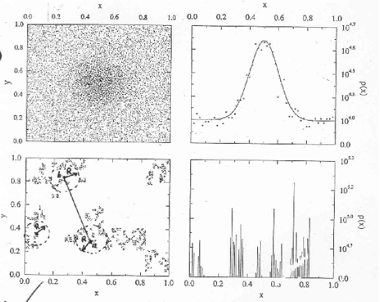
Figure 3: Top: an ordinary (fluid-like) discrete density field: a fluctuation on a Poisson background; bottom: a stochastic fractal density field (from Sylos Labini et al. 1998).

2.3.3 Fractal density fields

In the large scale structure analysis one applies a concept of discrete fractal point processes for which one may consider the density field in the form of a spatial distribution of $N$ particles in positions $\vec{x}_{a}$ with masses $m_{a}$ in a volume $V$, then

$$\rho(\vec{x})=\sum_{a=1}^{N}m_{a}\delta(\vec{x}-\vec{x}_{a})\,.$$ (20)

In the case of identical particles with $m_{a}=m$ one may simply use the concept of the number density field

$$n(\vec{x})=\sum_{a=1}^{N}\delta(\vec{x}-\vec{x}_{a})\,.$$ (21)

In order to describe the continuous hierarchy of clustering, which is a new characteristic of a fractal stochastic process, we first take into use a new independent variable, the radius $r$ of the spherical volume $V(r)$ in which the particles are counted. Then the fractal mass density may be defined as a function of two variables, the position $\vec{x}_{a}$ of a particle and the radius $r$ of the volume.

$$\rho_{{}_{\mathrm{fractal}}}=\rho(\vec{x}_{a},r)=\frac{M(\vec{x}_{a},V)}{V}\,,$$ (22)

where $M(\vec{x}_{a},V)$ is the mass inside the volume $V(r)$ located around the particle position $\vec{x}_{a}$.

For a mathematical infinite ideal fractal the number of points of the structure in a finite volume is infinite, so the mass is also infinite. In physics this problem may be avoided by some natural lower limit in sizes of elements, making the zero-level of the hierarchy. In this case one may speak about basic structure elements — point mass particles. Then the number of particles and the mass within the volume $V(r)$ is finite, i.e. in this case Eq.22 defines a physically measurable density. Though the quantity $\rho(\vec{x}_{a},r)$ is highly fluctuating from one particle position to another, as we shall see below it is possible to consider statistical average which is more stable characteristics of a fractal structure.

In Fig.3 an ordinary (fluid-like) density fluctuation on a Poisson background is compared with a stochastic fractal density fluctuations. In case of fractal structures the ordinary concept of the mass density of a continuous medium is not applicable. This is because the mass density can be defined only if both the position $\vec{x}$ and the volume $V$ are considered. In every volume $V$ containing a part of the structure there is a hierarchy of clusters and the value of the mass density strongly depends on the size of the volume. This is totally different from the usual calculus. Now there is no limit for the mass-volume ratio (Eq.13) and the density increases indefinitely when the volume tends towards zero:

$$\{\rho_{{}_{fractal}}\,\,\rightarrow\infty\,\,,\,\,\,\,\,\mathrm{for}\,\,\,\,\,V\rightarrow 0\}\,\,\,\,.$$ (23)

If the basic zero level elements exist then it determines the maximum value of the fractal density for the structure.

2.4 Exclusive properties of fractal density fields

2.4.1 Power-law density-radius relation

A characteristic feature of the fractal density field is a power-law behaviour of the density with increasing of the radius of the spherical volume $V(r)$ centered at a structure point. We can illustrate this property for the case of regular fractal structure (Fig.1), where the number of subelements within an element of the higher level is given by Eq.10. So in continuous representation, using Eq.22, one can define the fractal number density, which related to the elements of radius $r$, as

$$n_{V(r)}=\frac{N(r)}{V(r)}=\frac{3}{4\pi}Br^{-(3-D)}$$ (24)

where $D$ is the fractal dimension of the structure.

Hence, in order to calculate the fractal density one can start from a basic element which belongs to the structure and count the number of objects within the sphere $V(r)$ and divide it by the volume of the sphere $V(r)$ centered at the point. Apart from some fluctuation, depending on the actual position of the point within the structure the power-law Eq.24 will be obtained.

Note that the result is unexpected for our usual intuition — the density decreases from each point of the fractal structure. It seems like each point were the centre of the structure from which the density decreases outwards following the law in Eq.24. This property is essential for cosmological implications of the fractal structures (sec.6.5).

2.4.2 Massive, zero-density universes

An important consequence from Eq.24 is that in infinite space the fractal density field differs from an ordinary fluid-like density field at the limit of large volumes $V$ where

$$\{\rho_{{}_{fractal}}\,\,\rightarrow 0\,\,,\,\,\,\,\,\mathrm{for}\,\,\,\,\,V\rightarrow\infty\}$$ (25)

This property is due to a growing dilution of the hierarchy with increasing scales, so that a fractal structure is asymptotically dominated by voids.

Hence an infinite fractal universe can contain an infinitely large number of objects (hence an infinite mass) simultaneously with the zero density of the whole Universe. This unusual property of a hierarchical structure was exploited in old cosmological models to avoid gravitational and photometric paradoxes of the Newtonian infinite universe. This follows from the relations $\varphi\propto M/R$ and $F\propto M/R^{2}$.

2.4.3 The role of lower and upper cutoffs

In the realm of physics real structures usually have a lower scale $R_{\mathrm{min}}$ and an upper scale $R_{\mathrm{max}}$ between which the physical system follows fractal self-similar behaviour. These scales are called lower and upper cutoffs.

In studies of large-scale galaxy distribution the lower cutoff $R_{\mathrm{min}}$ is assumed to be equal to the size of a galaxy, while galaxies play a role of point-like particles. For different cosmological problems there could be different choices of the lower cutoff: dark matter clumps of $10^{6\div 8}M_{\odot}$, stars, comet-size objects, atoms, elementary particles. So the lower cutoff is usually a well-defined quantity.

The upper cutoff presents a much more complicated problem in studies of the galaxy distribution. In principle, one should apply such methods of the large scale structure analysis which allow one to determine directly from a galaxy survey the scale $R_{\mathrm{max}}=R_{\mathrm{hom}}$ where the galaxy distribution becomes homogeneous. However, such methods need a large survey volume whose size should correspond to several times the scale.

Up to now the largest galaxy redshift surveys cover a small part of the sky which hinders a firm estimation of the size $R_{\mathrm{hom}}$. Is there an upper cutoff for the large-scale galaxy distribution and what is its value? These are the primary questions around which the most acute discussion is going on.

2.4.4 Lacunarity

Two fractal structures with the same fractal dimension may look very different. In particular, when one makes fractal models of the galaxy distribution, it is quite essential how large a relative volume is occupied by voids, on a given scale.

This property was termed lacunarity by Mandelbrot (1982), from the word “lacuna” meaning hole or gap in Latin. Quantitatively lacunarity may be characterized by the constant of proportionality $F$ in the relation

$$N_{v}(\lambda>\Lambda)=F\Lambda^{-D}$$ (26)

where $N_{v}$ is the number of voids with size $\lambda>\Lambda$ within a fixed volume inside the structure.

Another definition was introduced by Blumenfeld & Mandelbrot (1997). They used the variation of the prefactor $B(\vec{x}_{a})$ in the density law computed for each structure point $\vec{x}_{a}$ within a ball with a fixed radius $R$, $N(r,\vec{x}_{a},R)=B(\vec{x}_{a},R)\,r^{D}$ (Eq.10). Then lacunarity is defined as a normalized dispersion of the distribution of the prefactor

$$\Phi=\frac{\langle(B-\bar{B})^{2}\rangle_{\vec{x}_{a}}}{\bar{B}^{2}}$$ (27)

Concrete examples of structures inside fixed sample volumes, having different lacunarities according to this definition may be found in Martinez & Saar (2002).

We note that the high lacunarity of the Rayleigh– Lévy flight fractal was the reason why it was rejected as a model for the real distribution of galaxies (Peebles 1980). However, later Mandelbrot (1998) demonstrated that fractal structures with a small lacunarity resemble more closely the arrangement of galaxies (see Fig.2).

2.4.5 Projection and intersection

The properties of orthogonal projections and intersections of a fractal structure play an important role in the analysis of galaxy samples with different geometries, both from angular 2-d and spatial 3-d catalogues.

Orthogonal projection. Let an object (structure) with a fractal dimension $D$, embedded in an Euclidean space of dimension $d=3$, be orthogonally projected onto an Euclidean plane with $d^{\prime}=2$. Then according to a general theorem of fractal projections (see Mandelbrot 1982; Falconer 1990), the projection as a fractal object receives the fractal dimension $D_{pr}$ so that

$$D_{pr}=D\,\,\,\,\mathrm{if}\,\,\,D<2$$ (28)

and

$$D_{pr}=2\,\,\,\,\mathrm{if}\,\,\,D\geq 2\,.$$ (29)

This means that in 3-d space a cloud having the fractal dimension $D\approx 2.5$ satisfies eq.29 and hence gives rise to a homogeneous shadow ($D_{pr}=2$) on the ground. Consequently, the orthogonal projection hides from view fractal structures with $D>2$. This has an important implication for the apparent distribution of galaxies on the sky (sec. 4.4).

Intersection of a fractal. If an object with a fractal dimension $D$, embedded in a $d=3$ Euclidean space, intersects an object with the dimension $D^{\prime}$, then according to the law of co-dimension additivity (see Mandelbrot 1982; Falconer 1990), the dimension of the intersection $D_{\mathrm{int}}$ becomes

$$D_{\mathrm{int}}=D+D^{\prime}-d\,.$$ (30)

For example, if a fractal structure with $D=2$ in 3-d space is intersected by a plane with $D^{\prime}=2$, then we obtain for the fractal dimension of the thin intersection $D_{\mathrm{int}}=2+2-3=1$. This property of intersections explains why a fractal structure with $D\approx 2$ may look as a fractal with $D\approx 1$ when inspected on large scales from a sample coming from a thin slice-like galaxy survey.

2.4.6 Multifractal structures

In fractal models of the galaxy distribution one usually utilizes only spatial positions for a sample of galaxies. This allows one to describe the distribution by means of only one parameter — the exponent in the power-law or the fractal dimension of the structure.

Real observational data contain also other important astrophysical information for each galaxy, such as luminosity, morphology, spectral properties, stellar contents e.t.c. In this case the scaling properties can be different for different types of galaxies. To take into account the dependence of the distribution on these parameters one has to introduce a more general model, called multifractal structures, which is characterized by a continuous set of fractal dimensions. Such approach was firstly suggested for galaxy distributions by Pietronero (1987). For recent discussions of this subject see Gabrielli et al. (2004), Martinez & Saar (2002) and Jones et al. (2004).

We note that multifractality may be viewed differently thanks to the complexity of the problem (even for fractals there is no unique definition). Multifractals are in contrast with homogeneity exactly like fractals are. In fact, the multifractal picture is a refinement and generalization of fractal properties (Paladin & Vulpiani 1987; Benzi et al. 1984).

2.5 Modern redshift and photometric distance surveys

For many years, astronomers could make only indirect conclusions about the distribution of galaxies on the basis of their two-dimensional projected locations on the celestial sphere. Such studies of projections are well reviewed in Peebles (1980).

In recent years the situation was completely changed when it became possible to measure the 3-dimensional distribution of galaxies using data from massive surveys of galaxy redshifts. At the present time there are several approaches for investigating the space distribution of matter (luminous and dark): photometric distance measurements, extensive redshift surveys of galaxies and quasars, the analysis of counts of galaxies, and the study of image distortion effects produced by weak gravitational lensing. All these observational studies have shown that clustering is a common phenomenon in the realm of nebulae.

2.5.1 Redshift surveys

Nature has given the astronomer, in the form of the linear redshift– distance law, an accurate way to measure extragalactic distances, which is generally more precise than photometric methods. For example, for a velocity dispersion of 50 km/s, typical for field galaxies, one can measure distances with an accuracy of about 1 Mpc. In order to get in this way a deep, 3-dimensional map of the surrounding galaxy universe, it is necessary to make deep surveys of redshifts, complete up to sufficiently faint magnitude limits.

Over 2700 galaxies had their redshift listed in the Second Reference Catalogue by de Vaucouleurs, de Vaucouleurs & Corwin (1976). This was the breakthrough which made it possible to use redshifts for mapping the structures made by galaxies.

Giovanelli & Haynes (1991) emphasized that ”In the last fifteen years, advances in detector and spectrometer technology at both optical and radio wavelengths have spurred a tremendous explosion in the galaxy redshift tally.” Indeed, this explosion has continued with an exponential rate up to present. Currently more than one million redshifts are known, almost all from optical spectra. This “redshift industry” continuously produces new points for the 3-d maps of spatial galaxy distribution. Special telescopes are dedicated to measurements of redshifts.

Table 1: Some recent galaxy surveys. The columns give: name of survey, solid angle $\Omega$ covered by survey, apparent magnitude limit, total number of galaxies $N$, the method of distance determination.

Catalogue	$\Omega$ ($sr$)	$m_{lim}$	$N$	distance	reference
				indicator
CfA1	1.83	14.5	1845	z	Huchra et al.1983
CfA2 (North)	1.23	15.5	6478	z	de Lapparent et al. 1988
PP	0.9	15.5	3301	z	Haynes & Giovanelli 1988
SSRS1	1.75	14.5	1773	z	Da Costa et al. 1990
SSRS2	1.13	15.5	3600	z	Da Costa et al. 1994
Stromlo-APM	1.3	17.15	1797	z	Loveday et al. 1992
LEDA	$4\pi$	16.0	25156	z	web site
LCRS	0.12	17.5	26000	z	Shectman et al. 1996
IRAS $2Jy$	$4\pi$	2. Jy	2652	z	Strauss et al. 1992
IRAS $1.2Jy$	$4\pi$	1.2 Jy	5313	z	Fischer et al. 1996
ESP	0.006	19.4	4000	z	Vettolani et al. 1997
KLUN	$4\pi$	15	6500	TF	Theureau et al. 1997b
KLUN+	$4\pi$	16	20000	TF	Theureau et al. 2004
Local Volume	$4\pi$	$<500$ km/s	300	RGS	Karachentsev et al. 2003
2dF	0.27	19.5	250 000	z	web site
SDSS	$\pi$	19	$10^{6}$	z	web site

Many extensive redshift surveys have already been completed, among them what are known by the abbreviations CfA, SSRS, LCRS, ESP. Their relevant parameters are presented in Tab.1. For a more detailed review the reader may consult Sylos Labini et al. (1998). Based on these surveys several 3-d maps of galaxy distribution have become available: both wide angle such as CfA1, CfA2, SSRS1, SSRS2, Perseus-Pisces, LEDA, and narrow angle such as LCRS, ESP.

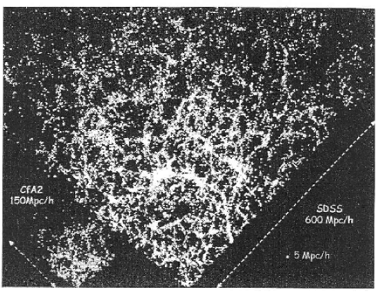
Figure 4: The large scale structure from the CfA and the first release of SDSS galaxy redshift survey (from Courtois et al. 2004a). One may easily recognize different kinds of structure on scales of about 100 Mpc.

The last decade saw the appearance of essentially larger surveys with hundreds of thousand of redshifts: the two-degree field galaxy redshift survey 2dF and the Sloan Digital Sky Survey SDSS. The depth of these galaxy catalogues allows one to detect and analyze structures with sizes up to 100 Mpc (see Fig.4).

Limits of a survey. A redshift survey is basically restricted by two limits: the apparent magnitude limit of the survey and the distance modulus limit which is different for different absolute magnitudes. In addition, it is important for the structure analysis to have a sufficiently large sky coverage.

The number of galaxies per square degree increases steeply with magnitude. There is roughly one galaxy/deg² up to $m\approx 15.5$ and about 85 up to 19 mag. On the other hand, this may be coped with the modern MOS (multiple object spectrograph) techniques which allow a simultaneous measurement of several tens of spectra of galaxies in the field of the telescope. Even if the sample is complete up to a certain apparent magnitude limit, its completeness in volume depends on the absolute magnitude: for galaxies with absolute magnitude $M$, the spatial completeness limit of the survey is at the distance modulus

$$\mu_{\mathrm{lim}}=m_{\mathrm{lim}}-M$$ (31)

For example, with $m_{\mathrm{lim}}=15.5$ and $M=-20$, $\mu=35.5$ which corresponds to the distance $r_{\mathrm{l}}=125$ Mpc (corresponding to $9300h_{{}_{75}}$ km/s). On the other hand, galaxies with $M=-18$ will be completely sampled only up to $r_{\mathrm{lim}}=50$ Mpc ($3700h_{{}_{75}}$ km/s). This shows that redshift surveys probe the distribution of only the most luminous galaxies at large distances, which may cause a biased picture. In order to cope with this problem, the only way is to push the surveys to fainter and fainter magnitude limits, because one cannot tell beforehand whether a galaxy taken is intrinsically bright or faint (or whether it is distant or relatively near).

2.5.2 Galaxy catalogues with photometric distances.

For the study of large-scale structure, redshift catalogues are generally superior to those based on photometric distances: 1) Redshift catalogues are much less time-consuming to make, 2) generally photometric distances are less accurate than redshift distances, and 3) redshifts may be measured for all Hubble types of galaxies.

However, there are questions which necessarily require large samples of galaxies for which both redshifts and independent photometric distances have been measured (e.g. the Hubble constant, deviations from the Hubble law, peculiar velocities and large scale streams). On the other hand, even photometric distances as such are valuable for investigating structures. They can be used for mapping the environment of the Local Group and for deriving the average number density law around us.

As radial velocities of galaxies, especially of those within groups and clusters, give only an approximate estimate of distances, Igor Karachentsev started a vast program of distance measurements to nearby galaxies, using the luminosity of their brightest blue and red stars (Karachentsev & Tikhonov, 1994; Karachentsev et al., 1997) and the luminosity of the tip of the red giant branch stars (Karachentsev et al. 2003). Over the last 10–15 years many nearby galaxies have been resolved into stars for the first time. This labour-consuming program requiring a lot of observing time with the largest ground-based telescopes, as well as the Hubble Space Telescope, is not yet complete. So far, the distances have been measured for about 150 galaxies situated within 9$h_{50}^{-1}$ Mpc (Karachentsev et al. 2003).

During the last years, a special effort has been undertaken to increase the Local Volume sample. “Blind” surveys of the sky in the 21 cm line (Kilborn et al. 2002), infrared and radio surveys of the Zone of Avoidance (Kraan-Korteweg & Lahav, 2000) and searches for new dwarf galaxies of very low surface brightness based on the POSS-II and ESO/SERC plates (Karachentseva & Karachentsev, 1998, 2000) have made the total number of the Local Volume galaxies increase more than two times.

A formidable example of a galaxy sample with photometric distances up to $\approx 100$ Mpc is the KLUN galaxy sample and its growing version KLUN+ (see KLUN+ home page at http://klun.obs-nancay.fr/KLUN+). These contain thousands of spiral galaxies for which both photometric magnitudes and the width of the neutral hydrogen 21cm line have been measured. Using the Tully–Fisher relation these two quantities (properly corrected and reduced to homogenized systems) allow one to make an estimate of the distance of a galaxy. Originally planned for measuring the value of the Hubble constant, the KLUN with its 5500 galaxies was used to study the radial number density distribution of galaxies around us (Teerikorpi et al. 1998). The new KLUN+ project is based on a Cosmological Key Project at the refurbished Nancay radio telescope in France. The HI survey plans to build a uniquely large magnitude-limited sample of 20 000 spiral galaxies distributed on the 80 percent of the sky visible from Nancay ($\delta>-40^{o}$). Theureau et al. (2004) give information and first results on the new HI measurements. The photometry comes from the DENIS (Near Infrared Survey) and 2MASS (2 Micron All Sky Survey). The aim is to build a sample complete to well defined magnitude limits in five photometric bands B, I, J, H and K (the earlier KLUN had only B magnitudes and diameters).

All these data give us the possibility to study the large scale galaxy distribution by means of different statistical methods which we describe below.

2.5.3 How to discover fractal structures

From the 3-d map shown in fig.4 (SDSS) one may recognize by eye structures with different sizes up to 100 Mpc. However, a quantitative analysis of the observed inhomogeneities in the spatial distribution of galaxies is a hard problem around which there is going on the debate on fractality of observed structures.

In order to understand the meaning of conclusions from different analyses of the observational data, it is highly advisable to investigate idiosyncracies and limitations of the used methods. The next section addresses this issue and discusses main mathematical tools used to discover fractal structures. We restrict our consideration to the methodological questions arising in practical applications of the methods to analysis of galaxy samples.

3 Statistical methods to detect fractality in galaxy distribution

Several statistical methods have been used for the analysis of both 2-d (angular distributions) and 3-d (spatial distributions) galaxy catalogues. A comprehensive review of mathematical approaches for the description of the large scale galaxy distribution may be found in the book by Martinez & Saar (2002).

Here we confine our discussion to the fractal approach. Detailed descriptions of such methods for the analysis of the distribution of galaxies are given by Sylos Labini et al. (1998) and Gabrielli et al. (2004).

One of our goals is to compare the standard method of the $\xi$ correlation function (Peebles, 1980; 1993) with the fractal approach (Pietronero 1987; Gabrielli et al. 2004). We demonstrate that it is essential for the study of the distribution of galaxies to utilize mathematical instruments which are adequate for the existing structures. It is especially important to use undistorted estimators for measuring the fractal dimension and the range of fractality.

3.1 Definitions for correlation functions

The theory of stochastic processes introduces and studies different functions intended for the correlation analysis (see e.g. sect.2 of Gabrielli at al. 2004).

3.1.1 Complete and reduced correlation functions

The complete two-point correlation function $R_{\mu\mu}$ (we call it simply the complete correlation function) of a stationary isotropic process $\mu(\vec{r})$ is defined as

$$R_{\mu\mu}(r)=\langle\mu(\vec{r}_{1})\mu(\vec{r}_{2})\rangle$$ (32)

where $r=\mid\vec{r}\mid=\mid\vec{r_{1}}-\vec{r_{2}}\mid$ is the mutual distance between considered points, and $\langle\cdot\rangle$ is the ensemble average over all realizations of the stochastic process.

Taking into account the truly constant mean value $\mu_{0}$ of the process

$$\mu_{0}=\langle\mu(\vec{r})\rangle=\mathrm{const}$$ (33)

one may define the reduced two-point correlation function $C_{2}$ for the fluctuations around $\mu_{0}$ (we call it simply the reduced correlation function) as

$$C_{2}(r)=\langle(\mu(\vec{r}_{1})-\mu_{0})(\mu(\vec{r}_{2})-\mu_{0})\rangle=R_{\mu\mu}(r)-\mu_{0}^{2}\,.$$ (34)

For $r=0$ it expresses the squared dispersion of the process as $\sigma_{\mu}^{2}=C_{2}(0)$.

We emphasize an important difference between the complete and reduced correlation functions $R_{\mu\mu}(r)$ and $C_{2}(r)$. For a stochastic process with long range power-law correlations the complete correlation function $R_{\mu\mu}(r)$ has a power-law form, while the reduced correlation function $C_{2}(r)$, according to its definition (eq.34), cannot be a power law in this case.

3.1.2 Mass variation in spheres and characteristic scales

In the applications that we discuss the stochastic process $\mu(\vec{r})$ will describe the density field $\rho(\vec{r})$.

Conditional and unconditional functions. It is important to distinct between conditional and unconditional functions (or statistics). For instance, when one considers such statistics which are defined with the condition that there is a fixed point-particle relative to which other particles of a process are considered, then one speaks about a conditional function. We will see below that the two major tools of the LSS analysis, the $\Gamma$ and $\xi$ functions, are both conditional correlation functions.

As an example of unconditional statistics we consider mass (number) fluctuations inside a sphere of radius $R$. Let us define in addition to $\rho(\vec{r})$ a new stochastic variable $M(R)$ as

$$M(R)=\int_{V(R)}\rho(\vec{r})d^{3}r$$ (35)

For a given radius $R$ fluctuations of this mass calculated in different positions in space can be characterized by the normalized mass variance $\sigma^{2}_{M}(R)$:

$$\sigma^{2}_{M}(R)=\frac{\langle M(R)^{2}\rangle-\langle M(R)\rangle^{2}}{\langle M(R)\rangle^{2}}\,\,,$$ (36)

where

$$\langle M(R)\rangle=\frac{4\pi}{3}\rho_{0}R^{3}$$ (37)

and for volume $V=V(R)$

$$\langle M(R)^{2}\rangle=\int_{V}d^{3}r_{1}\int_{V}d^{3}r_{2}\langle\rho(\vec{r}_{1})\rho(\vec{r}_{2})\rangle$$ (38)

Here there is no condition on the locations of the centre of the sphere, which may be put anywhere in the space within the sample regardless of the positions of the particles, also “between” them.

The scale of homogeneity. Our intuitive vision of uniformity may be formalized by means of the variable $M(R)$. E.g. the homogeneity scale $R_{\mathrm{hom}}$ may be defined as the scale at which $\sigma^{2}_{M}(R_{\mathrm{hom}})=1$ (or some other threshold value). This means that it is possible to regard a distribution of particles as approaching homogeneity if the average mass fluctuation within spheres of radius $R_{\mathrm{hom}}$ is about the average mass $\langle M(R_{\mathrm{hom}})\rangle$. This scale is well defined when $\sigma^{2}_{M}(R)\rightarrow 0$ for $R>R_{\mathrm{hom}}$.

The correlation length. The second scale is the correlation length $R_{\mathrm{cor}}$, which does not depend on the amplitude of the correlation function and just characterizes the rate of decrease of the correlation function. The correlation length may be infinite, as it is for a power law correlation $R_{\mu\mu}(r)\propto r^{-\gamma}$, or finite, as for an exponential correlation function $R_{\mu\mu}(r)\propto e^{-r/R_{\mathrm{cor}}}$.

3.2 The method of the $\xi$-correlation function

A widely used classical approach to the analysis of the large scale structure is the method of correlation function. It was first introduced to the galaxy analysis by Totsuji & Kihara (1969) who adopted this method from the statistical physics of ordinary gas density fluctuations (e.g. Landau & Lifshitz 1958). It was further developed and extensively applied to galaxy data by Peebles (1980, 1993) and others (for recent reviews see Martinez & Saar 2002; Jones et al. 2004).

3.2.1 Peebles’ $\xi$-correlation function

According to Peebles (1980) the two-point correlation function $\xi(r)$ is defined as the dimensionless reduced correlation function of the density fluctuations $\delta\rho(\vec{r})=\rho(\vec{r})-\rho_{0}$ around the average density $\rho_{0}$

$$\xi(r)=\frac{\langle\delta\rho(\vec{r}_{1})\delta\rho(\vec{r}_{2})\rangle}{\rho_{0}^{2}}=\frac{\langle\rho(\vec{r}_{1})\rho(\vec{r}_{2})\rangle-\rho_{0}^{2}}{\rho_{0}^{2}}$$ (39)

In fact the $\xi$-function is simply the reduced correlation function (eq.34) divided by the squared mean value of the process (eq.33), i.e.

$$\xi(r)=C_{2}(r)/\rho_{0}$$ (40)

In the case of a distribution of identical particles (with masses $m=m_{0}$) one uses a number density $n(\vec{r})=\rho(\vec{r})/m_{0}$, whose average is $\langle n(r)\rangle=n_{0}$. Then

$$\xi(r)=\frac{\langle n(\vec{r}_{1})n(\vec{r}_{1}+\vec{r})\rangle}{n_{0}^{2}}-1\,.$$ (41)

This dimensionless function measures correlations of fluctuations relative to a constant average number density $n_{0}$.

In the theory of stochastic processes one usually considers a normalized correlation function which is defined as $K_{\mu\mu}(r)=C_{2}(r)/\sigma_{x}^{2}=(R_{\mu\mu}(r)-x_{0}^{2})/\sigma_{x}^{2}$. Then there is the normalization condition $K_{\mu\mu}(0)=1$. The definition for the $\xi$-function (eq.39) implies the condition $\xi(0)=\sigma_{\rho}^{2}/\rho_{0}^{2}$.

Definition via Poisson process. The correlation function may also be defined as a measure of the deflection of a distribution of particles from a Poisson (uniform) distribution (Peebles 1980). In this case one considers two infinitesimal spheres at the points $\vec{r}_{1}$ and $\vec{r}_{2}$ with volumes $dV_{1}$ and $dV_{2}$ and with the mutual distance $\vec{r}_{12}$. Then the joint probability to find one particle in the volume $dV_{1}$ and another particle in the volume $dV_{2}$ is proportional to the number of pairs $dN_{12}$

$$dN_{12}=n_{0}^{2}dV_{1}dV_{2}[1+\xi(\vec{r}_{12})]\,,$$ (42)

where $n_{0}$ is the ensemble average number density of particles and $\xi(\vec{r}_{12})$ measures the deflection from the Poisson distribution. This definition implies that $\xi(\vec{r}_{12})=0$ automatically for a Poisson process.

For a statistically isotropic distribution the function $\xi(\vec{r}_{12})=\xi(r)$ depends on the separation $r$ only. For the case when an object is chosen at random from the sample, the probability of finding that it has a neighbour at a distance $r$ in $dV$ (e.g. $4\pi r^{2}dr$) is proportional to the expected number of neighbours $dN$

$$dN=n_{0}dV[1+\xi(r)]\,.$$ (43)

Here $\xi(r)$ is considered as the same two-point correlation function as defined by eq.41 (see sect.33 of Peebles 1980). It is a measure of finding an excess number of particles relative to the Poisson distribution, at the distance $r>0$ provided that there is a particle at $r=0$.

3.2.2 $\xi$-function estimators

In the theory of stochastic processes it is important to make a distinction between functions (e.g. $\xi(r)$) defined by ensemble averages and their estimators ($\hat{\xi}(r)$), e.g. applied to a finite galaxy sample.

To estimate the two-point correlation function from an available data sample of $N_{s}$ objects within a volume $V_{s}$, one generally uses a method based on artificially generated Poisson process, which fills the same volume $V_{s}$ of the sample. Then the $\xi$-function for a given scale $r$ is estimated as the ratio of the number of pairs with such mutual distance in the sample to the number of such pairs in the artificial Poisson distribution. There are several different pairwise estimators (Kerscher et al. 2000; Martinez & Saar 2002; Gabrielli et al. 2004), and the difference between them lies mainly in their method of edge correction.

For instance, the Davis–Peebles estimator weights the points according to the part of the spherical shell volume which is contained in the volume of the sample. It has the form

$$\hat{\xi}(r)=\left(\frac{N_{rd}}{N_{s}-1}\right)\frac{N_{p}(r)}{N_{p,rd}(r)}-1\,,$$ (44)

Here $N_{p}(r)$ is the number of data-data pairs of observed objects in the catalogue having their mutual distance in the interval $(r,\,r+dr)$. $N_{p,dr}(r)$ comes from the joint catalogue of data and artificial random distributions in the same volume $V_{s}$. It is the number of data-random pairs with the distance $r$ in the joint catalogue. $N_{s}$ and $N_{rd}$ are the total numbers of objects in the real sample and the random distribution, respectively.

An essential assumption of the correlation function method is the hypothesis of homogeneity according to which the true average of objects $n_{0}$ is estimated from the observed sample as

$$\hat{n}_{0}=\bar{n}=\frac{N_{s}}{V_{s}}$$ (45)

with a high formal accuracy $\sigma_{n_{0}}\approx 1/\sqrt{N_{s}}$, where $N_{s}$ is the total number of objects in the volume $V_{s}$ of the “fair” sample, which is assumed to be representative of the homogeneous distribution of galaxies in the whole Universe.

3.2.3 The normalization condition for $\xi$ estimators

A significant point related to $\xi$-function estimators was emphasized by Pietronero (1987) and Calzetti et al. (1988), and in more detail by Gabrielli et al. (2004). Namely, the definition of the correlation function as a deflection from the Poisson distribution (eq.43) implies an integral condition for the $\xi$ function estimated from a finite sample of galaxies.

This comes from the fact that for any sample with a finite number of galaxies $N_{s}$ in a volume $V_{s}$ the estimation of the average number density is $\bar{n}=N_{s}/V_{s}$. Integrating the left side of eq.43 over the sample volume we get

$$\int_{V_{s}}dN=N_{s}-1$$ (46)

where $N_{s}-1$ is the number of neighbours, i.e. the total number of particles in the volume $V_{s}$ without the one whose neighbours are counted. Then the integration of the right side of eq.43 over the sample volume gives

$$N_{s}-1=\int_{V_{S}}\bar{n}dV+\bar{n}\int_{V_{S}}\hat{\xi}(r)dV.$$ (47)

The first term on the right side is $\int_{V_{s}}\bar{n}dV=N_{s}$, the total number of the particles in the sample. Hence the second term will satisfy the condition

$$\int_{V_{S}}\hat{\xi}(r)dV=-\frac{1}{\bar{n}}$$ (48)

or in dimensionless form:

$$\int_{V_{S}}\hat{\xi}(r)\frac{dV}{V_{s}}=-\frac{1}{N_{s}}$$ (49)

In the case of fluid-like correlated distributions the effective number density of particles may be arbitrarily large and hence the condition of eq.48 becomes

$$\int_{V_{S}}\hat{\xi}(r)dV=0$$ (50)

These restrictions lie behind some controversial results obtained by the $\xi$ function method of the large scale structure analysis. In particular, we have in mind the inevitable non-power law behaviour of the $\xi$ estimator. From eqs.48 and 50 follows that there is a distance $r_{z}$ where $\hat{\xi}(r_{z})=0$. Here the correlation function estimator changes its sign from positive to negative values, which is impossible for a power-law function.

3.2.4 A systematic distortion of the true power-law correlation due to the $\hat{\xi}$-estimator

As was shown above, if the complete correlation function is a power-law then neither $\xi(r)$ nor $\hat{\xi}(r)$ can be a power-law function. Nevertheless, in practice $\hat{\xi}(r)$ is usually presented in the form

$$\hat{\xi}(r)=\left(\frac{r}{r_{0}}\right)^{-\gamma}\;,\;\;\;r_{1}<r<r_{2}\,,$$ (51)

valid for some range of scales $r_{1}<r<r_{2}$. Here the parameter $r_{0}$ defines the amplitude.

From such a power-law presentation one usually derives two numbers: the unit scale $r_{0}$ and the correlation exponent $\gamma$. We emphasize that due to the normalization condition (eq.49) both numbers give systematically distorted values for the homogeneity scale and the power-law exponent of the true complete correlation function $R_{\mu\mu(r)}$ describing the density field.

The unit scale $r_{0}$ (which is often called, somewhat misleadingly, as correlation length) is defined from the relation

$$\hat{\xi}(r_{0})=1\,,$$ (52)

which characterizes the amplitude of density fluctuations at the scale $r_{0}$. In fact, it is a distorted value of a true homogeneity scale of the process if the true value is equal to or larger than the size of a maximum sphere embedded completely in the sample volume $V_{s}$.

The correlation exponent $\gamma$ in the power-law representation of $\hat{\xi}(r)$ (eq.51) describes correctly only a restricted interval of scales $r_{1}<r<r_{2}$ . On scales $r>r_{2}$ this does not represent the true value of the exponent, because there the estimated value is distorted as the normalization condition (eq.49) makes $\hat{\xi}(r)$ deflect from the inherent power-law and to cross zero level. For example, below it will be shown that for the exponent $\gamma$ is derived twice the true correlation exponent at the unit scale $r_{0}$ (sect. 3.4.1).

On scales $r<r_{1}$ the true value of the exponent is distorted due to the noise of discreteness, which behaves as $\sigma\propto r^{-3/2}$ (eq.19). The error will essentially increase for scales smaller than the average distance between particles in a sample (e.g. $r<\lambda_{0}$). We will see later examples of how this has happened in data analysis.

3.2.5 Redshift-space and the peculiar velocity field

From a galaxy redshift survey one obtains a redshift-space map, i.e. ($\alpha$ , $\delta$, $z_{\mathrm{obs}}$) coordinates, where ($\alpha$ , $\delta$) give the position on the sky and $z_{\mathrm{obs}}$ gives the observed redshift of a galaxy in the sample. The value of $z_{\mathrm{obs}}$ in principle contains all possible contributions from different physical causes according to the relation

$$1+z_{\mathrm{obs}}=(1+z_{\mathrm{cos}})(1+z_{v})(1+z_{\phi})(1+z_{\mathrm{new}})$$ (53)

Here $z_{\mathrm{cos}}$ is the cosmological redshift which determines the true distance to the galaxy $r_{gal}(z)$ calculated from the empirical distance–redshift relation (i.e. from the Hubble law, which gives $r_{\mathrm{gal}}=cz_{\mathrm{cos}}/H_{0}$) or from an adopted cosmological model for large redshifts. The $z_{v}$ is the redshift component caused by the peculiar velocity of the galaxy, $z_{\phi}$ is the gravitational part of the redshift caused by the local gravitational potential of the galaxy (e.g. in a cluster), and $z_{\mathrm{new}}$ is a possible component due to unknown cosmological physics.

Distance error due to peculiar velocity. Let us consider the influence of the peculiar velocity field on the distance estimation. For peculiar velocities $v<<c$ the Doppler part of the observed redshift is determined by the radial component $v_{r}$ of the velocity as

$$z_{v}\approx v_{r}/c\,\,.$$ (54)

So for small radial peculiar velocities $v_{r}$ we obtain

$$z_{\mathrm{obs}}=z_{\mathrm{cos}}+\frac{v_{r}}{c}(1+z_{\mathrm{cos}})$$ (55)

Hence the true spatial galaxy distribution will be distorted by a peculiar velocity field in the line of sight direction

$$r_{\parallel\mathrm{obs}}=r_{\parallel}+\Delta r_{v}$$ (56)

by the value

$$\Delta r_{v}=\frac{v_{r}(1+z_{\mathrm{cos}})}{H_{0}}=5\mathrm{Mpc}\,h^{-1}_{100}\frac{v_{r}(1+z_{\mathrm{cos}})}{500\mathrm{km/s}}$$ (57)

Note that the factor $(1+z_{\mathrm{cos}})$ leads to an increasing influence of $v_{\mathrm{pec}}$ on the distance distortion for deep redshift surveys.

Real-space and redshift-space $\xi$ functions. A directly observed $\xi$-function is called the redshift-space correlation function $\xi_{z}(s)$. In order to obtain the real-space correlation function $\xi_{\mathrm{real}}=\xi(r)$ one should extract and delete all non-cosmological contributions to $z_{\mathrm{obs}}$. This is a hard problem because it requires a priori knowledge of the peculiar velocity field, the total mass around the galaxy, and restrictions on new physics.

The shape of the observed $\xi_{z}(s)$ is determined by the character of the peculiar velocity field. In virialized clusters the velocity dispersion leads to the so-called “fingers-of-God” effect, i.e. an elongated shape along the line of sight direction $r_{\parallel}$. The mean tendency of galaxies at larger scales to approach each other due to the gravity of large-scale structures will appear as a compression of $\xi_{z}(s)$ in the direction $r_{\parallel}$. As these two effects are related to different spatial scales, they do not compensate each other.

Peebles (1980; sec.76) and Davis & Peebles (1983) suggested a procedure for the restoration of both the true $\xi(r)$ and the relative peculiar velocity distribution $f(v)$ from the observed correlation function $\xi_{z}(r_{\perp},r_{\parallel\mathrm{obs}})$ where $r_{\perp}$ an $r_{\|\mathrm{obs}}$ are the observed perpendicular and parallel to the line of sight components of the separation $s=\sqrt{r_{\perp}^{2}+r_{\parallel\mathrm{obs}}^{2}}$.

Derivation of the real-space $\xi$-function. The method is based on the calculation of the projected correlation function $w(r_{\perp})$ which does not depend on the peculiar velocity field, if the distribution of the radial peculiar velocities is symmetrical around each galaxy of the sample. Then integrating along the line of sight we obtain:

$$w(r_{\perp})=2\int_{0}^{\infty}\xi_{z}(r_{\perp},r_{\parallel obs})dr_{\parallel obs}\,,$$ (58)

where in practice the interval of integration is restricted by chosen radial velocity limits. Then the wanted inverse is the Abel integral

$$\xi(r)=-\frac{1}{\pi}\int_{r}^{\infty}\frac{w^{\prime}dr_{\perp}}{(r^{2}-r_{\perp}^{2})^{1/2}}\,,$$ (59)

where $w^{\prime}=dw(r_{\perp})/dr_{\perp}$. Eq.59 gives the solution for the problem of restoration of the real-space $\xi(r)$ correlation function.

For the power law $\xi=(r_{0}/r)^{\gamma}$ the integral (58) gives

$$w(r_{\perp})=Ar_{\perp}^{1-\gamma}\,,$$ (60)

where

$$A=r_{0}^{\gamma}\frac{\Gamma_{e}(1/2)\Gamma_{e}((\gamma-1)/2)}{\Gamma_{e}(\gamma/2)}$$ (61)

and $\Gamma_{e}(x)$ is the Euler gamma function.

Limitations of the projection method. It is clear from eq.60 that such a solution for the real-space $\xi$ correlation function is valid only if the exponent $\gamma\geq 1$. For example, $\gamma=1$ gives $w(r_{\perp})=$ constant, which demonstrates that a uniform background galaxy distribution may be confused with the projection of real-space non-uniform distribution.

According to the theorem on fractal projections (sec.2.4.5) such a method inevitably leads to elimination of information on structures with the fractal dimension $D\geq 2$. Therefore to take into account the peculiar velocity field within fractal structures with $D\geq 2$ (such a structure is actually observed, see sec.5), it is necessary to use another method of restoration for the correlation function, which is free from the above limitation. Also a more careful study of distance errors in both $r_{\parallel}$ and $r_{\perp}$ components is required.

Estimation of the relative velocity dispersion. In the case, when density and velocity fields are weakly coupled, the observed correlation function $\xi_{z}(s)$ can be modelled as a convolution of the real space correlation function $\xi(r)$ with the galaxy pairwise velocity distribution $f(v)$. According to Peebles (1980, sec.76) and Davis & Peebles (1983) this equation may be presented in the form

$$1+\xi_{z}(r_{\perp},r_{\parallel\mathrm{obs}})=H_{0}\int\left[1+\xi(\sqrt{r_{\perp}^{2}+r_{\parallel}^{2}})\right]f(v)dr_{\parallel}$$ (62)

where

$$v=H_{0}r_{\parallel\mathrm{obs}}-H_{0}r_{\parallel}+\bar{v}_{12}(r)$$ (63)

and $\bar{v}_{12}(r)$ is the mean radial pairwise velocity of galaxies at separation $r$, which is represented by a model. Davis & Peebles (1983) adopted the model

$$\bar{v}_{12}(r)=\frac{H_{0}r_{\parallel}}{1+(r/r_{0})^{2}}$$ (64)

and an exponential form for $f(v)$:

$$f(v)=B~{}\exp\left(-2^{1/2}\mid v\mid/\sigma_{12}\right)$$ (65)

As a result of this approach one obtains the pairwise velocity dispersion $\sigma_{12}$.

3.3 The method of conditional density

3.3.1 Definitions

The method of conditional density has been successfully used for analysis of fractal structures in modern statistical physics. This method was proposed for extragalactic astronomy by Pietronero (1987) and has been applied to 3-d galaxy catalogues by many authors (see reviews in Coleman, Pietronero 1992; Sylos Labini, Montuori, Pietronero 1998; Gabrielli et al. 2004). Conditional density method has the advantage that it gives an undistorted estimation of the true power law correlation and the true fractal dimension. It also may be used for finding an undistorted value of the homogeneity scale of a galaxy sample.

Continuous stochastic processes. The conditional density $\Gamma(r)$ may be defined by means of the complete correlation function (eq.32) in the following form:

$$\Gamma(r)=\frac{R_{\mu\mu}(r)}{\mu_{0}}=\frac{\langle\rho(\vec{r}_{1})\rho(\vec{r}_{1}+\vec{r})\rangle}{\rho_{0}}$$ (66)

Here $\rho(\vec{r})$ is the stochastic density field and $\rho_{0}$ is the ensemble average density. The $\Gamma$-function has the physical dimension of density [g/cm³], and it is a measure of correlation in the total density field without subtraction of the average density. The physical dimension of the $\Gamma$ function agrees with the common interpretation of $\Gamma(r)$ as an average density law around each point of the structure. This makes its estimator a natural detector of fractality.

As we shall see below this definition allows one to construct such an estimator which has no additional restrictions like the normalization in eq.48, and hence is able to give an undistorted value of the exponent for true power-law correlations.

Discrete stochastic fractal processes. Let us consider a discrete stochastic process, one realization of which is a set of identical particles at randomly selected positions $\{\vec{x}_{a}\},~{}a=1,...,N$, so that the number density $n(\vec{x})$ is given by the expression

$$n(\vec{x})=\sum_{a=1}^{N}\delta(\vec{x}-\vec{x}_{a})\,.$$ (67)

If the stochastic process generates a fractal, then it is natural to define the number density as a function of two variables: $n=n(\vec{x},r)$. The first variable describes the position $\vec{x}_{a}$ of a structure particle, and the second variable gives the radius $r$ of a ball inside which one calculates the number of particles of the structure. The variable $r$ serves for constructing a statistics which can measure the strength of the singularity around a particle of the fractal structure where the number of particles grows as a power-law $N(r)\propto r^{D}$.

Denote by $N_{V}(\vec{x}_{a},r)$ the number of particles in a sphere of radius $r$, centered at the particle $a$ with the coordinates $\vec{x}_{a}$, belonging to the structure:

$$N_{V}(\vec{x}_{a},r)=\int_{0}^{r}n(\vec{x_{a}}+\vec{x})4\pi x^{2}dx\,,$$ (68)

and $N_{S}(\vec{x}_{a},r)$ is the number of particles in the spherical shell $r,r+\triangle r$, with the centre at $\vec{x}_{a}$:

$$N_{S}(\vec{x}_{a},r)=\int_{r}^{r+\triangle r}n(\vec{x_{a}}+\vec{x})4\pi x^{2}dx\,.$$ (69)

From one realization to another these quantities fluctuate, but after averaging over many realizations the stable power-law dependence on the scale $r$ emerges. In the case of ergodic processes averaging over many realizations may be replaced by many points in one realization. Following the work by Pietronero (1987) we define the conditional (number) density of a stochastic fractal process in the form:

$$\Gamma(r)=\left\langle\frac{N_{S}(\vec{x}_{a},r)}{4\pi r^{2}\triangle r}\right\rangle_{\vec{x}_{a}}=\frac{DB}{4\pi}~{}r^{-(3-D)}\,,$$ (70)

and the conditional volume density as

$$\Gamma^{*}(r)=\left\langle\frac{N_{V}(\vec{x}_{a},r)}{(4\pi/3)r^{3}}\right\rangle_{\vec{x}_{a}}=\frac{3B}{4\pi}~{}r^{-(3-D)}\,,$$ (71)

where $\langle\cdot\rangle_{\vec{x}_{a}}$ means averaging over all points $\vec{x}_{a}$ in one realization with the condition that the centres of the spheres lie at the particles of a realization (this explains the word “conditional”). The last equalities in (70) and (71) relate to ideal fractal structures, for which

$$\Gamma^{*}(r)=\frac{3}{D}\Gamma(r)$$ (72)

3.3.2 $\Gamma$-function estimator.

Consider a stochastic fractal process where the number of particles $N_{V}(\vec{x}_{a},r)$ in a sphere of radius $r$, centered at the point $\vec{x}_{a}$ and the number $N_{S}(\vec{x}_{a},r)$ of particles in the shell ($r,r+\triangle r$) are given by eqs.68 and 69. Taking into account definitions of conditional densities (eqs. 70 and 71) one can use following two statistics for their estimation from one realization (a finite galaxy sample):

$$\hat{\Gamma}(r)=\frac{1}{N}\sum_{a=1}^{N}\frac{1}{4\pi r^{2}\triangle r}\int_{r}^{r+\triangle r}n(\vec{x_{a}}+\vec{x})4\pi x^{2}dx$$ (73)

for the shell conditional density $\Gamma$, and

$$\hat{\Gamma}^{*}(r)=\frac{1}{N}\sum_{a=1}^{N}\frac{3}{4\pi r^{3}}\int_{0}^{r}n(\vec{x_{a}}+\vec{x})4\pi r^{2}dx$$ (74)

for the volume conditional density $\Gamma^{*}$. So the use of the conditional density method is in principle quite simple, just counting the number of particles inside the spherical volume $V(r)$ or inside the shell $S(r)\Delta r$. This is done for each structure point and then the average is calculated. For the $\Gamma$-function estimation one need not generate artificial Poisson distributions, which was necessary for the $\xi$-function method.

Fractal dimension and co-dimension. For a fractal structure both the $\Gamma$ function (eq.70) and the estimator (eq.73) have a power-law form

$$\hat{\Gamma}(r)=\Gamma_{0}r^{-\gamma}$$ (75)

This very important property of the $\Gamma$-estimator allows one to obtain an undistorted value of the fractal dimension in a galaxy sample.

The exponent that defines the decay of the conditional density

$$\gamma=D-3$$ (76)

is called the co-dimension, where $D$ is the fractal dimension (or the correlation dimension $D_{2}$). The amplitude $\Gamma_{0}$ of the estimator $\hat{\Gamma}(r)$ does not change when the sample volume $V_{s}$ is increased, only the range of available scales $r$ increases. This corresponds to the meaning of $\Gamma(r)$ as characterizing the number density behaviour.

Homogeneity scale. For a fractal structure which has an upper cutoff at a homogeneity scale $R_{\mathrm{hom}}$, after which the distribution becomes uniform, the fractal dimension $D=3$, and the estimator of the $\Gamma$-function is

$$\hat{\Gamma}(r)=\mathrm{constant},\,\,\,\,\mathrm{for}\,\,\,r>R_{\mathrm{hom}}\,\,.$$ (77)

Thus the method of conditional density is a powerful instrument when one searches for the crossover from the regime of fractal clustering to the realm of homogeneity.

So, for processes with a finite upper cutoff scale of fractality, beyond which the distribution of particles turns into homogeneity, the statistics (73) and (74) give constant values corresponding to the fractal dimension $D=$ 3 as it indeed should be for uniform structures.

3.3.3 Redshift-space $\Gamma_{z}(s)$ and $v_{pec}$

As we discussed in sec.3.2.5 an estimation of the spatial distribution of galaxies from redshift catalogues is based on the redshift-space ($\alpha$ , $\delta$, $z_{obs}$). Using the same notations as in sec.3.2.5 for the $\xi$ function ($s$, $r_{\perp}$, $r_{\parallel}$) we can right for the redshift-space conditional density

$$\Gamma_{z}(s)=\Gamma_{z}(r_{\perp},r_{\parallel\mathrm{obs}})\,\,.$$ (78)

The relation between the real-space $\Gamma(r)$ and redshift-space $\Gamma_{z}(s)$ conditional density is

$$\Gamma_{z}(r_{\perp},r_{\parallel\mathrm{obs}})=\int g(\vec{r},\,\vec{w})\Gamma(r)d^{3}w\,\,,$$ (79)

where $\vec{w}=\vec{v}_{1}-\vec{v}_{2}$ is the relative peculiar velocity of a galaxy pair at separation $\vec{r}$, and $g(\vec{r},\,\vec{w})$ is the relative peculiar velocity distribution. Here the components of the relative distance $\vec{r}$ are given by the following formulae: $r_{1}=r_{\perp}$, $r_{3}=r_{\parallel\mathrm{obs}}-w_{3}/H_{0}$, and $r^{2}=r_{\perp}^{2}+(r_{\parallel\mathrm{obs}}-w_{3}/H_{0})^{2}$.

In order to restore the real-space conditional density from the directly observed redshift-space conditional density it is necessary to make computer simulations of artificial fractal structures with known peculiar velocity fields and then compare the modelled redshift-space $\Gamma_{\mathrm{mod}}(s)$ with the observed $\Gamma_{z}(s)$.

3.3.4 $\Gamma$-function for 2-d intersections

If in 3-d space a fractal structure is intersected by a plane then the expected value of the fractal dimension for the intersection is given by eq.30:

$$D_{\mathrm{int}}=D-1$$ (80)

To make the $\Gamma$-function analysis for the sample which presented the 2-d intersection we shall use the 2-d coordinate system $\vec{y}=(y_{1},\,y_{2})$ for which we can calculate the $\Gamma$-function for the intersection $\Gamma_{\mathrm{int}}(y)$.

Such a situation may occur in a slice-like galaxy survey for scales $r$ larger than the thickness of the survey. E.g. for the true fractal dimension $D=2$ the fractal dimension of the intersection will be $D_{\mathrm{int}}=1$. Hence we expect to obtain a power-law behaviour of the corresponding $\Gamma_{\mathrm{int}}(y)\propto y^{-1}$. We will see below that the intersection theorem helps one to understand the behaviour of the power-spectrum derived from slice-like galaxy surveys.

3.4 Comparison of correlation function and conditional density

3.4.1 The relation between $\Gamma$ and $\xi$.

From the definitions of the conditional density $\Gamma$ (eq.66) and correlation function (eq.41) we have the relation:

$$\xi(r)=\frac{\Gamma(r)}{n_{0}}-1$$ (81)

if the average number density $n_{0}$ of a considered stochastic process exists. Both $\Gamma$ and $\xi$ functions are conditional characteristics of a stochastic process, i.e. they are defined on the condition that the centres of counting spheres are set to structure particles. However, there is still a deep difference between them. The $\Gamma(r)$ represents the complete correlation function, while the $\xi(r)$ represents the reduced correlation function of the stochastic process. This fact makes the properties of the corresponding $\xi$ and $\Gamma$ estimators very different. Finally, it results in conflicting values for the estimated correlation exponent and homogeneity scale of a galaxy sample.

From eq.81 follows a similar relation between the estimators for a finite sample of galaxies:

$$\hat{\xi}_{FS}(r)=\frac{\hat{\Gamma}_{FS}(r)}{\bar{n}}-1$$ (82)

Here $\hat{\xi}_{FS}$ is called the “full shell” estimator because it is defined through the $\Gamma$ estimator which is calculated using full shells completely embedded in the sample volume.

The estimator $\hat{\Gamma}$ (eq.73) is always a positive function and has a power-law form for fractal structures. On the contrary, the estimator $\hat{\xi}$ (eq.44) inevitably changes its sign and hence cannot be presented as a power law even for scale invariant structures. All estimators of the $\xi$-function, which are based on counting of pairs relative to an artificial Poisson distribution, have a common drawback. They give essentially distorted values for the true correlation exponent of the complete correlation function of long range power-law correlated processes and for fractal distributions. But the $\Gamma$-function estimator is specially constructed in order to give undistorted values of the correlation exponent and fractal dimension.

The $\Gamma$-function estimator relates to intrinsic properties of the sample, while the $\xi$-function estimator depends on both intrinsic and external properties of the sample. In fact, $\hat{\Gamma}$ measures the behaviour of the total density inside spheres within a sample, while $\hat{\xi}$ measures density fluctuations relative to the average density, which is assumed to be valid for all space outside a finite sample. This can be illustrated also by the following reasoning. Let us consider counts around a fixed point. The expected number of points in a shell with radius $r$ and volume $dV$ is $n(r)dV$, where $n(r)$ is the conditional density $\Gamma(r)$ describing the density–radius law. On the other hand, the same expected number may be calculated with the correlation function $\xi(r)$ as $n_{0}(1+\xi(r))dV$. So

$$\Gamma(r)=(1+\xi(r))n_{0}$$ (83)

It is important to note that the right-hand side of eq.83 becomes defined only after the mean density $n_{0}$ is calculated for the whole sample, while $\Gamma(r)$ always exists locally. Remember that $\xi(r)$ was defined for fluctuations around the mean $n_{0}$.

Fractal density field. For the case of a scale-invariant stochastic fractal density field, the complete correlation function $\Gamma(r)$ has the power-law form

$$\Gamma(r)=\frac{BD}{4\pi}\;r^{-\gamma}\,\,,$$ (84)

while for the same fractal structure the reduced correlation function $\xi(r)$ will be

$$\xi(r)=\frac{BD}{4\pi n_{0}}\;r^{-\gamma}-1$$ (85)

which is not a power-law. This difference between complete and reduced correlation functions was pointed out by Pietronero & Kuper (1986).

Thus the $\xi$-function may be approximated by a power-law only for such $r$ when $\xi(r)\gg 1$, which corresponds to small scales $r<<r_{0}$. However, on small scales the noise of discreteness is essential, which also leads to distortion of a true power-law. Hence a $\xi$-function estimation gives a distorted values of the correlation exponent not only on large scales (normalization), but also on small scales (discreteness).

It is instructive to calculate the exponent $\gamma_{\xi}$ of the correlation function (eq.85) on scales close to the unit scale $r_{0}$. Taking the logarithmic derivative of eq.85 one obtains (Joyce, Montuori, Sylos Labini 1999):

$$\gamma_{\xi}(r)=-\frac{d[\log\xi(r)]}{d\log r}=\frac{2\gamma(r/r_{0})^{-\gamma}}{2(r/r_{0})^{-\gamma}-1}$$ (86)

Therefore at the unit scale $r=r_{0}$ we get the remarkable result:

$$\gamma_{\xi}(r_{0})=2\gamma$$ (87)

For example, for a true density power-law with $\gamma=1$, one would infer an apparent slope $\gamma_{\xi}=2$ for the correlation $\xi$-function, if measured at scales close to the “correlation length” $r_{0}$!

3.4.2 The dependence of $r_{0}$ on sample depth.

The sample depth $R_{s}$ is an important global parameter of an observed galaxy distribution. For a fractal structure sampled inside a spherical volume $V_{s}=\frac{4\pi}{3}R_{s}^{3}$ with $\bar{n}=N_{s}/V_{s}=3BR_{s}^{D-3}/4\pi$, the eq.85 yields

$$\hat{\xi}(r)=\frac{D}{3}\left(\frac{r}{R_{s}}\right)^{-\gamma}-1\,\,,$$ (88)

and the unit scale $r_{0}$ comes to depend on the sample parameters.

Inserting $r=r_{0}$ into eq.81 and taking into account that $\xi(r=r_{0})=1$ one gets

$$r_{0}=\left(\frac{DB}{8\pi\bar{n}}\right)^{1/\gamma}$$ (89)

where $\bar{n}$ is the average number density of objects in the sample. Hence one obtains:

$$\Gamma(r_{0})=\frac{DB}{4\pi}\;r_{0}^{D-3}=2\bar{n}=\frac{6B}{4\pi}R_{s}^{D-3}$$ (90)

From this follows a simple relation between the correlation length $r_{0}$ and the depth of the sample $R_{s}$:

$$r_{0}=\left(\frac{3-\gamma}{6}\right)^{1/\gamma}R_{s}$$ (91)

We note again that this is true for a spherical sample (i.e. $R_{s}=R_{max}^{sph}$) and a fixed luminosity (i.e. $L=const$) of sample galaxies.

3.4.3 Geometry of a survey and characteristic scales.

A strong restriction for the practical application of the $\Gamma$-function method is the requirement that there should be room for the whole sphere in the volume of the considered sample. For example, for galaxy surveys with slice-like geometry, this makes it impossible to measure the conditional density for scales larger than the thickness of the slice, i.e. the diameter of the maximum sphere fully contained in the survey volume.

The above dependencies between $r_{0}$ and various sample parameters were derived for the ideal case of a simple fractal in a sufficiently large spherical volume inside which the correlation function is estimated. For a non-spherical survey geometry (like a slice or cone) these relations are valid only for such scales $r$ for which the survey galaxies are contained completely within the sphere with the radius $r$. For non-spherical geometries these dependencies are expected to differ from the above predictions.

For a galaxy sample under consideration one should always control the following characteristic distance scales:

$$R_{sep},\,\,R_{max}^{sph},\,\,R_{s}\,.$$ (92)

The separation distance $R_{sep}$ between galaxies in a sample may be roughly estimated as $\bar{n}^{-1/3}$ or calculated from the nearest neighbours distribution. We may define $R_{sep}=\alpha R_{sep-av}$, where $\alpha\approx 0.1$ and $R_{sep-av}$ is the average distance between nearest neighbours in a sample. For $r<R_{sep}$ the discreteness noise is important.

The radius of the maximum sphere $R_{max}^{sph}$ is related to the complete embedded sphere in the sample and play a crucial role in estimation of correlation properties of the galaxies from the sample. The depth $R_{s}$ of a survey is related to the largest distances of galaxies in the sample, it essentially differs from the radius of the maximal sphere in the case of a slice-like surveys.

As a general rule for a correlation analysis of slice-like samples one should consider separately two regions of scales. First,

$$R_{sep}<r<R_{max}^{sph}\,\,,$$ (93)

where it is possible to use the $\Gamma$ function method and estimate the value of the true fractal dimension, and secondly,

$$R_{max}^{sph}<r<R_{s}\,\,,$$ (94)

where the $\Gamma$ function cannot be applied. In this region other methods should be developed such as the $\Gamma$ function for fractal intersections and the two-point conditional column density.

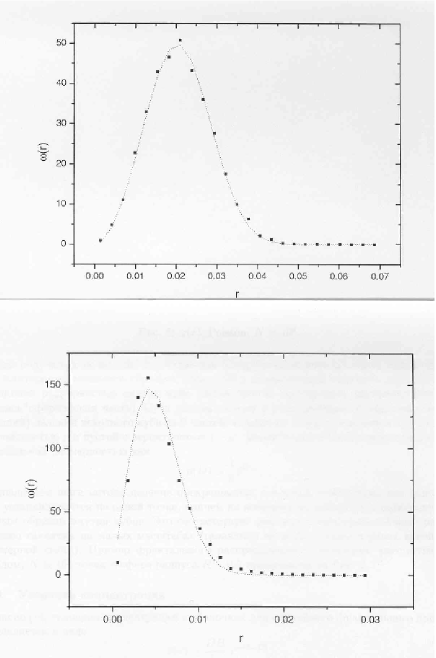
Figure 5: Probability distributions for finding the nearest neighbour at a distance $r$ for two cases:(top) the homogeneous Poisson distribution ($D=3$) and (bottom) a fractal distribution with $D=2$ (a random Cantor set). The distributions are in 3-d space inside a sphere of diameter = 1, the total number of points in each case is $N=2.5\cdot 10^{3}$. The dotted curves correspond to theoretical predictions according to eqs. 99, 100 (from Vasiliev 2004).

3.5 Nearest neighbours distribution.

The distribution of distances to the nearest neighbour point is a useful property of fractals, which may be used to make a distinction between fractal and ordinary distributions. It is discussed in detail by Gabrielli et al. (2004).

Poisson distribution. For example, for a Poisson process in 3-d space the probability density distribution $\omega(r)$ for finding the nearest neighbour at a distance $r$ is

$$\omega(r)=4\pi n_{0}r^{2}\exp\left(-\frac{4\pi n_{0}r^{3}}{3}\right)\;.$$ (95)

For Poisson process the average distance between point-particles is $R_{sep}\approx n_{o}^{-1/3}$

Fractal distribution. There is no exact formulae for the general case of a fractal structure. However, Gabrielli et al. (2004) derived a useful approximation for the probability density distribution for the nearest neighbour in a fractal structure:

$$\omega(r)=4\pi Cr^{D-1}\exp\left(-\frac{4\pi Cr^{D}}{D}\right)\;,$$ (96)

where $C=DB/4\pi$.

Figure 5 presents $\omega(r)$ for two cases: a homogeneous Poisson distribution ($D=3$) and a fractal distribution with $D=2$. The dotted curves correspond to theoretical predictions from eq.95 and eq.96. It is seen that the lower is the value of the fractal dimension $D$, the closer are the neighbours within the fractal structure. This example shows that the nearest neighbour probability function may be used as an additional method for estimating the fractal dimension of a galaxy sample.

3.6 Two-point conditional column density

3.6.1 Definitions

The conditional densities of stochastic fractal processes above discussed were one-point, as the centre of the sphere in which particles are counted lies at one fixed point $\{a\}$ with the coordinates $\{\vec{x}_{a}\}$ and the counts are made around each point $\{a\}$ of the sample. However, in some cosmological studies, e.g. related to gravitational lensing (Baryshev & Ezova 1997), it becomes necessary to use two-point conditional densities, whereby one simultaneously fixes two particles $\{a,~{}b\}$ with the coordinates $\{\vec{x}_{a},~{}\vec{x}_{b}\}$ and counts galaxies within a thin cylinder between these points.

In order to define the distribution of particles along such a cylinder, whose axis connects two structure points $\{a,~{}b\}\subset\{\vec{x}_{i}\,,\,i=1,...,N\}$, Baryshev & Bukhmastova (2004) introduced the concept of 2-point conditional column density $\eta_{ab}(r)$ for a stochastic fractal process. In applications to galaxies, according to the cosmological principle of Mandelbrot the particles $a$ and $b$ are statistically equivalent, hence for each of them the 1-point conditional density is given by the expression (70), which is proportional to the probability of finding particles at the distance $r$ from fixed structure points.

Let us now take two independent points of the structure at the distance $r_{ab}=|\vec{x}_{a}-\vec{x}_{b}|$ from each other. Denote by $C$ the event, when particles appear at the distance $r_{a}$ from $a$ and independently at the distance $r_{b}$ from $b$. Then $C$ is given by the union $C=A\bigcup B$ of the two events related to $a$ and $b$. So the 2-point conditional column density, which is proportional to the probability of finding particles around the particles $a$ and $b$, may be presented as a sum of 1-point conditional densities. The assumption of independent events is a first approximation. Numerical simulations have shown that this approximation is sufficient for the analysis of usual fractal structures (Baryshev & Bukhmastova 2004). Then the 2-point conditional column density can be expressed as

$$\eta_{ab}(r)=\frac{1}{2}\left[\Gamma_{a}(r)+\Gamma_{b}(r_{ab}-r)\right]$$

$$=\frac{DB}{8\pi}\cdot~{}r_{ab}^{-\gamma}\cdot\left[\left(\frac{r}{r_{ab}}\right)^{-\gamma}+\left(1-\frac{r}{r_{ab}}\right)^{-\gamma}\right]\,,$$ (97)

where $\gamma=\mathrm{D}-3$. The distance $r$ is measured along the segment of the line connecting the particles $a$ and $b$, and at the same time it defines the radius $r$ of the sphere having its centre at the first point and the radius $r_{ab}-r$ for another sphere having its centre at the second point. The constant $B$ defines the normalization. We note that in this formula the volume elements are taken along the line connecting the two points – in this sense the coordinate $r$ is not a spherical radial coordinate, but a Cartesian coordinate labelling volume elements (“tablets”) with thickness $dr$ along this cylinder.

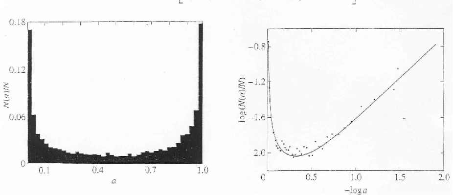
Figure 6: (left) The observed distribution of the galaxy two-point conditional column density $\hat{\eta}_{ab}(r)$ of the LEDA sample along cylinders with $l<100$ Mpc. (right) The same distribution in logarithmic scale and the fitted theoretical curve $\eta_{ab}(r)$, with the fractal dimension $D=2.02$ (from Baryshev and Bukhmastova 2004).

3.6.2 Estimation

In order to estimate $\eta_{ab}(r)$ one may use the statistic

$$\hat{\eta}_{ab}(r)=\left\langle\frac{N_{c}(\vec{x}_{a},\vec{x}_{b},~{}r,~{}h,~{}\triangle r)}{\pi h^{2}\triangle r}\right\rangle_{\{a,b\}}$$

$$=\frac{1}{N_{ab}}\sum_{\{a,b\}}^{N_{ab}}\frac{1}{\pi h^{2}\triangle r}\int_{r}^{r+\triangle r}\int_{0}^{h}n(\vec{x})2\pi h~{}dh~{}dr\,,$$ (98)

where $N_{c}$ is the number of particles in a volume element of the cylinder with a diameter $h$ and height $\triangle r$ and whose axis connects the structure particles $a$ and $b$. The volume element lies at the distance $r$ from $a$, which corresponds to the distance $r_{ab}-r$ from $b$. Averaging is performed for every pair of particles with connecting cylinders having the length in the interval $(l,l+\Delta l)$. The parameters $h$ and $\Delta r$ are chosen to be a fraction of the mean separation of the particles in the sample. Practical modelling of artificial fractals show that the estimated fractal dimension is robust to reasonable variations of the tablet size (Baryshev & Bukhmastova 2004; Vasiliev 2004).

A more general situation, which may be encountered in practice, is that both a fractal structure and a homogeneous background exist in the sample.Then the practical calculation of the fractal dimension $D$ by means of the estimator $\eta_{ab}(r)$ may be done by fitting through the observations the dimensionless probability distribution with three free parameters $\gamma,\,R_{1},\,R_{2}$

$$\frac{N(y)}{N}=R_{1}\cdot\frac{[y^{-\gamma}+(1-y)^{-\gamma}]}{2}+R_{2}$$ (99)

where $N(y)$ is the observed number of points which are found in each tablet, i.e. within the small intervals $(y,y+\Delta y)$ along the cylinder with a length $l$. The variable $y$ is the relative distance measured along the line connecting the two points ($y=r/r_{ab}=r/l$). $N$ is the total number of points within cylinders of length $l$. In the case of genuine self- similar structures it is possible to calculate these numbers for all cylinders of different length simultaneously. $R_{2}$ shows the contribution of a possible Poisson background.

It is useful to introduce a measure of the relative strength $\beta$ of the fractal component as was done by Vasiliev (2004):

$$\beta=\frac{1-R_{2}}{R_{2}}\;.$$ (100)

When $\beta=1$, the contribution from a fractal structure is equal to the Poisson background contribution ($R_{2}=0.5$).

The main advantage of the cylinder method is that it can work for slice-like surveys allowing the study of scales comparable to the depth of the survey.

3.7 Fourier analysis of the galaxy distribution

3.7.1 Ordinary density fields

If the spatial distribution of objects is given by a stochastic density field, then fluctuations of this field may be represented by the Fourier integral as a superposition of plane spatial waves with the wave number $k=|\vec{k}|=2\pi/\lambda$:

$$\delta(\vec{x})=\frac{\varrho(\vec{x})-\bar{\varrho}}{\bar{\varrho}}=\frac{1}{(2\pi)^{3}}\int\tilde{\delta}(\vec{k})e^{-i\vec{k}\cdot\vec{x}}d^{3}k\,$$ (101)

Here the Fourier transform $\tilde{\delta}(\vec{k})$ of the density fluctuations $\delta(\vec{x})$ is a complex quantity and thus may be given in the form

$$\tilde{\delta}(\vec{k})=|\tilde{\delta}(\vec{k})|\exp(i\phi(\vec{k}))\,.$$ (102)

Here we see that for a complete description of the spatial distribution of objects the analysis should include both the amplitude spectrum $|\tilde{\delta}(\vec{k})|$ and the phase spectrum $\phi(\vec{k})$.

In the case of a Gaussian random process the phases of plane waves are distributed uniformly in the interval $[0,\,2\pi]$ and to describe the density field it is sufficient to consider only the power spectrum

$$P(\vec{k})=\langle|\tilde{\delta}(\vec{k})|^{2}\rangle\,.$$ (103)

When the distribution is isotropic, the power spectrum and the correlation function are connected by the relation

$$P(k)=4\pi\int\xi(r)\frac{\sin(kr)}{kr}r^{2}dr\,.$$ (104)

Thus for a power law correlation function $\xi(r)\propto r^{-\gamma}$ the power spectrum has also a power law form $P(k)\propto k^{\gamma-3}$ for restricted range of scales $k_{1}<k<k_{2}$. For small $k$ (large scales $\lambda>R_{s}$) there is a limit due to the size of a survey $R_{s}$, which give $P(k)\rightarrow 0$ for $\lambda\rightarrow R_{s}$.

The phase spectrum $\phi(\vec{k})$ carries important information, complementary to $P(k)$. Possible non-Gaussianity of the clustering properties i.e. non-uniformity of the phase spectrum was considered in Chiang & Coles 2000 and Coles & Chang 2000.

The main problem of the power spectrum analysis is the same as for the correlation function: the average density $\bar{\rho}$ should be well defined within the sample volume.

However an advantage of the $P(k)$-method is that the correlation exponent $\gamma$ may be estimated without distortion from $P(k)$ for the scales $\lambda<R_{max}^{sph}$.

3.7.2 Fractal density fields

For stochastic fractal processes one may perform the Fourier-analysis of fractal density field ( Sylos-Labini & Amendola 1996, Sylos Labini et al. 1998). They introduced the concept of generalized power spectrum $\Pi(k)$ of a fractal process, which is defined by the Fourier transformation of the conditional density $\Gamma(r)$:

$$\Pi(k)=4\pi\int\Gamma(r)\frac{\sin(kr)}{kr}r^{2}dr\,.$$ (105)

Because of a power-law form $\Gamma(r)\propto r^{-(3-D)}$ for the conditional density of a stochastic fractal process, we also get for the generalized power spectrum a power law $\Pi(k)\propto k^{-D}$. Here $D$ is the fractal dimension, which hence may be directly measured from the power spectrum. The generalized power spectrum is a suitable tool for describing highly irregular systems with fractal properties.

3.7.3 Role of geometry of a sample

In the case of a slice-like survey for scales larger than maximum sphere completely embedded in the sample, the geometry of considered structure become effectively be close to the case of an intersection of a 3-d fractal structure by a plane. Hence according to the theorem on intersections of fractals (sec.2.4.5) it is expected that for a structure with the true fractal dimension $D$ the measured fractal dimension of the sample will be $D_{int}=D-1$. It means that there are three characteristic intervals of scales for behaviour of power spectra $P(k)$ or $\Pi(k)$: 1) for scales $\lambda<R_{max}^{sph}$ we get $P(k)\propto k^{-D}$ with exponent equal the true fractal dimension; 2) for scales $R_{max}^{sph}<\lambda<R_{s}$ we get $P(k)\propto k^{-(D-1)}$ with exponent equal the fractal dimension of intersection; and 3) for scales $\lambda>R_{s}$ we get $P(k)\rightarrow 0$ due to a finite size of the sample.

3.8 Multifractals and luminosity function

3.8.1 Spectrum of fractal dimensions

There are several different definitions for the fractal dimension: Hausdorf dimension $D_{H}$, box or capacity dimension $D_{b}$, correlation dimension $D_{2}$, mass-length dimension $D_{m}$ (for brief descriptions for astronomers see e.g. Gabrielli et al. 2004; Martinez & Saar 2002). For self-similar distributions all these dimensions are usually equal (and are $\leq d$, the dimension of the embedding space). In such simple cases we shall use the symbol $D$ for this common fractal dimension. For multifractal analysis which operates with a whole spectrum of fractal dimensions all dimensions should be considered separately.

We have already encountered the mass-length fractal dimension $D_{m}$ in the Fournier world model which was constructed so that $M(r)\propto r$ and hence $D_{m}=1$. It was the first mathematical model of a regular fractal structure applied to the whole universe.

The box dimension or capacity of a set $S\subset\Re^{p}$ is defined as

$$D_{b}=\lim_{\epsilon\rightarrow 0}\frac{\log N(\epsilon)}{\log(1/\epsilon)}$$ (106)

where $N(\epsilon)$ is the minimum number of p-dimensional boxes of size $\epsilon$ needed to cover completely the set $S$.

In the case of spatial galaxy distribution $p=3$ and one should extract from a sample the cube (3-d box) within which to perform the calculation of the box dimension $D_{b}$. The slope of the plot of $\log N(\epsilon)$ versus $\log(1/\epsilon)$ gives an estimation of the box dimension.

The correlation dimension $D_{2}$ is defined via the correlation exponent $\gamma$ in the complete correlation function or conditional density $\Gamma$. Our discussion in the previous section was intended to distinguish between homogeneity and scale invariant properties and, for this purpose, it remains perfectly appropriate even if the galaxy distribution were multifractal. In this case the correlation functions we have considered would correspond to a single exponent of the multifractal spectrum, but the issue of homogeneity versus scale invariance (fractal or multifractal) is exactly the same.

We emphasize also that a discussion in the literature around the multifractal properties of galaxy distribution had its origin in the difference between the values of the fractal dimension obtained by two methods: box-counting and correlation function (Jones et al. 1988; Martinez & Jones 1991; Martinez & Saar 2002). However, as we have seen above, the difference was caused by the use of the $\xi$-function estimator which gave a distorted value for the correlation dimension $D_{2}$. If one uses the appropriate $\Gamma$-function estimator then the unique fractal dimension $D\approx 2$ well fits observational data and hence eliminates the claimed need for that kind of multifractality.

3.8.2 Luminosity function

Above we considered fractal structures made of identical particles with unit mass. In connection with galaxies, Sylos Labini et al. (1998) and Gabrielli et al. (2004) use the term multifractality in the case where the so-called fractal support (positions of particles) has a unique dimension. In this case a stochastic process labels the fractal support particles by different values of some random quantity $\mu$ (for example luminosity $L$ or mass $m$).

Real galaxies have different masses and different luminosities which may be characterized by a luminosity function $\phi(L)$. This is usually represented by Schechter’s law

$$\phi(L)~{}dL=\phi^{*}\cdot(L/L^{*})^{\alpha}\cdot exp(-L/L^{*})~{}dL\,,$$ (107)

which gives the fraction of galaxies in the unit volume in the luminosity interval $(L,~{}L+dL)$. The parameters $\alpha$ and $L^{*}$ are to be determined from observations and $\phi^{*}$ is the normalizing coefficient from the condition $\int_{\beta}^{\infty}\phi(L)~{}dL=1$, so that

$$\phi^{*}=\frac{\Gamma(\alpha+1,~{}\beta)}{L^{*}}\,.$$ (108)

Here $\Gamma(n,~{}x)$ is the incomplete gamma function and $\beta$ is a parameter which determines the luminosity truncation in the faint tail.

3.8.3 Space-luminosity correlation

Let us consider a realization of a stochastic process for which one may define the luminosity (or mass) density $\mu$ in the form

$$\mu(\vec{x})=\sum_{i=1}^{N}\mu_{i}~{}\delta(\vec{x}-\vec{x}_{i})\,.$$ (109)

where $\mu_{i}$ is the luminosity (or mass) of $i$-th particle.

Pietronero (1987), Coleman & Pietronero (1992) and Sylos-Labini & Pietronero (1996) regard luminosity or mass density functions as multifractal measures on the set of realizations. Multifractals are characterized by the spectrum of fractal dimensions $D(L)$ which determines the dependence of the fractal dimension on luminosity or mass. This means that luminous and faint galaxies may have different spatial distributions. One prediction of the multifractal model is that the fractal dimension decreases for increasingly luminous objects.

Let $N_{L,S}(\vec{x}_{a},~{}L,~{}r)$ be the number of galaxies having the luminosity in the interval $(L,~{}L+\triangle L)$ in a spherical shell $S(r)=4\pi r^{2}\triangle r$ with its centre at the point $\vec{x}_{a}$ belonging to the structure. In order to generalize the concept of conditional density to the case of particles of different luminosity or mass, we define the conditional luminosity (mass) density as

$$\nu(L,r)=\left\langle\frac{N_{L,S}(\vec{x}_{a},L,r)}{4\pi r^{2}\triangle r~{}\triangle L}\right\rangle_{\vec{x}_{a}}=$$ (110)

$$=\frac{1}{N}\sum_{i=1}^{N}\frac{1}{4\pi r^{2}\triangle r~{}\triangle L}\int_{L}^{L+\triangle L}\int_{r}^{r+\triangle r}\mu(\vec{x})d^{3}x~{}dL\,.$$ (111)

As shown by Sylos-Labini & Pietronero (1996)for a wide class of multifractal stochastic processes the conditional luminosity density has the general form

$$\nu(L,r)=\phi_{{}_{r}}(L)\cdot\Gamma_{{}_{L}}(r)=$$ (112)

$$\phi^{*}\cdot\left(\frac{L}{L^{*}(r)}\right)^{-\alpha}\cdot\exp(L/L^{*}(r))\cdot\frac{D(L)B}{4\pi}\cdot~{}r^{D(L)-3}\,.$$ (113)

This means that the Schechter law for the luminosity function is an observable consequence of multifractality and not just a convenient analytical form!

Special features of the expression (113) are the dependence of the “knee” of the LF, $L^{*}(r)$, on the radius of the volume and also the dependence of the fractal dimension on luminosity $D(L)$. These properties may be used for testing multifractality. However, this needs large samples of galaxies, because fractal analysis must be made for each luminosity interval separately. If the distribution is multifractal then the brightest luminosity $\>L_{\mathrm{max}}$ in a sample is related to its spherical depth $\>R_{s}$ by the relation (Coleman & Pietronero 1992)

$$L_{\mathrm{max}}\propto R_{s}^{\beta}\,\,,$$ (114)

where the exponent $\beta$ depends on multifractal spectrum.

4 The epoch of angular-position galaxy catalogues

The history of main events illuminating the fractal debate in the 20th century is presented in the Tab.2 ”The debate on large scale fractality”. This subject has always been at the centre of cosmological thinking, even sharp debates, because of its direct link to cosmological principles. Of course, inhomogeneities in our neighbourhood are evident and the border to the assumed uniformity must lie somewhere at a larger distance. During the history the border to uniformity has gradually shifted outwards from the crystal sphere of fixed stars to Newton’s evenly scattered stars, and then to Hubble’s uniform galaxy distribution. At our times the observed superclusters of galaxies have put the border of uniformity to a scale of at least 100 Mpc.

Table 2: The history of the debate on large scale fractality.

Years	Authors	Subject
1900 –	Fournier d’Albe	regular hierarchical models
1920s	Charlier, Selety, Lundmark	criteria for infinite world
paradoxes	Einstein, Selety	Mach, stability, middle point
	Shapley, Zwicky, Abell	strong galaxy clustering
1930s –	Carpenter, Kiang, Karachentsev	superclusters up to 100 Mpc
1970s	Neyman, Scott	2-level hierarchical model
	de Vaucouleurs	cosmic density-radius law
clusters		$\rho(r)\propto r^{-\gamma}$ with $\gamma=1.7$
and	———————————–	————————————–
uniformity	Hubble	uniformity from galaxy counts
		$\log N(m)=0.6m+$ constant
	Ambartsumian, Holmberg, Fesenko	variable extinction in MW
	Sandage, Tammann, Hardy	linear Hubble law at $<30$ Mpc
	Webster, Longair	isotropy of radio sources
	Wertz, Bonnor, Wesson, Alfven	physics of hierarchy
1970s –	Haggerty, Severne, Prigogine	N-body dynamics in hierarchies
1980s	Totsuji, Kihara, Peebles	$w\propto\theta^{-0.8}\Rightarrow\xi\propto r^{-1.8}$
	Mandelbrot	fractals, multifractals
$\xi$	Baryshev, Perdang	first evidence for $D=2$:
and	Lerner, Schulman, Seiden	$M(r)$, $z(r)$, stability, percolation
$\Gamma$	———————————-	——– —————————-
function	Davis, Peebles	$\gamma=1.8$, $r_{0}=5$ Mpc, 2000 galaxies
	Einasto, Klypin, Kopylov, Bahcall	$r_{0}$ depends on depth and type
	Pietronero	the method of $\Gamma$ function
	Pietronero, Sanders, Coleman	the first fractal analysis of CfA
	Pietronero, Ruffini, Calzetti et al.	explanation of $r_{0}(R_{s})$
	Jones, Martinez, Saar, Einasto	$D_{2}=1.2$, $D_{0}=2$, multifractal?
	Sylos Labini, Montuori, Pietronero	$D\approx 2$ from all 3-d catalogs
1990s –	Wu, Lahav, Rees	fractality at $r<30$ Mpc
2000s	Teerikorpi, Hanski, Theureau et al.	TF $<200$ Mpc $\Rightarrow D=2.2$, KLUN
	Paturel, Teerikorpi, Courtois	LEDA counts $<15^{m}$: $0.44m$, $D=2.2$
fractals	Baryshev, Bukhmastova	2-point column density: $D=2.1$
in	Zehavi (SDSS team)	$\xi(s)\propto s^{-1.2}$, 29 300 gal.
3-d maps	Hawkins (2dFGRS team)	$\xi(s)\propto s^{-0.75}$, 200 000 gal., $D=2.25$
		distortion by peculiar velocities?
	Gott et al. (SDSS team)	500 Mpc Sloan Great Wall

Together with the border to homogeneity, the centre of the universe has moved from the earth to the sun, and to the Milky Way. One of the most famous events in 20th-century astronomy was the Great Debate between Harlow Shapley and Heber D. Curtis in 1920 about the scale and structure of the Universe (Smith 1983). In fact, this debate heralded the change of the Milky Way into an ordinary galaxy, whereby the centre of the universe finally disappeared into the realm of galaxies.

Meanwhile, a new debate around the nature of galaxy clustering and on the border of the large scale inhomogeneity emerged. For almost the whole 20th century this struggle was going on, involving such figures as Charlier, Einstein, Selety, Hubble, Lundmark, de Vaucouleurs, Sandage, Peebles and others. As always in astronomy and in particular in this new extragalactic field, the scarcity of available observations at any historical moment leads to uncertain interpretations of the data. The modern phase of this fractal debate concerns observational tests with specially dedicated galaxy surveys to find the spatial scale where homogeneity becomes reality.

New aspects and instruments for tackling the inhomogeneity problem entered the scene, when the concept of fractal was introduced by Benoit Mandelbrot (1975, 1977, 1982, 1988). Fractals, self-similar structures with long-range correlations, had been disclosed in physics and were then extended to astronomical scales, from the solar system and interstellar clouds to clusters of galaxies. Fractals on the largest scales became observable entities thanks to new astronomical techniques for measuring redshifts for thousands of galaxies, together with theoretical recipes for powerful data analysis. The primary open questions are: 1) Where is the border of transition from fractality to homogeneity?, and 2) what is the value of the fractal dimension of the galaxy distribution?

4.1 The birth of the debate

4.1.1 Einstein – Selety correspondence

In his first paper on cosmology Einstein (1917) gave arguments for homogeneity. He notes that any finite stellar system will evaporate into infinity due to internal gravitational interactions. He also emphasized that stellar velocities are small, which spoke against large potential differences and supported uniform large scale mass distribution. For Einstein a strong theoretical argument was that the Poisson equation modified by a cosmological constant term $\lambda$

$$\triangle\phi-\lambda\phi=4\pi G\rho$$ (115)

has a solution for the density $\rho=$ constant:

$$\phi=-\frac{4\pi G}{\lambda}\rho,$$ (116)

so that a static, homogeneous matter distribution is possible, which also explains the small stellar velocities. The homogeneity scale was supposed to be about the mean distance between stars.

In his paper Einstein then extended this result to general relativity, obtaining the spherical world model with a finite radius of curvature. At the end of his article Einstein’s mentions that he does not ponder if his model is compatible with available astronomical observations. Later this crucial hypothesis of homogeneity came to be called Einstein’s cosmological principle of homogeneity.

The Austrian scientist Franz Selety was aware of both Einstein’s homogeneous and Charlier’s hierarchical models. In an article in Annalen der Physik, Selety (1922) argued that it is possible to construct hierarchical worlds which fulfil simultaneously the following conditions:

• infinite space

• infinite total mass

• mass filling space so that locally there is everywhere a finite density

• zero average density of the mass in the whole world

• non-existence of a unique middle point or middle region of the world

In fact, Selety was one of the first to realize that the cosmological principle of “no centre” may also be valid for hierarchical systems. He expressed the essence of hierarchic models in that the universe appears for an observer in a “molecular-hierarchic” system everywhere basically similar. He also raised the question of Mach’s principle in such universes and argued that it can be fulfilled. He pointed out that in such models a zero average density for the whole universe exists simultaneously with its infinite total mass.

Einstein (1922) quickly replied to Selety. He expressed his opinion that Mach’s principle is not fulfilled in a zero-density universe. Selety (1923) did not agree with Einstein and once more discussed the crucial points of his model. Summarizing the arguments which were raised by Einstein and Selety, we see as main objections to hierarchical models in the 1920’s:

• Mach’s principle is not valid for a hierarchic world model with zero global density.

• Large potential differences in a strongly inhomogeneous universe lead to too high a velocity dispersion for stars, which is not observed.

• A hierarchic stellar system will evaporate and stars will fill the voids, leading to a homogeneous distribution.

• A hierarchic world contains a preferred middle point.

4.1.2 A retrospective view on the posed questions.

In retrospect, one may say that intriguingly, all these arguments are still actual in modern cosmology.

First, Mach’s principle links the inertial mass of a body to the large scale mass distribution in the universe. Only relative to those distant masses one can define the acceleration of a test particle. In fact, the nature of inertial mass is still a challenge for modern theoretical physics, including general relativity, where the rest mass of a particle is regarded as a relativistic invariant, independent of the cosmologically distributed mass around the particle. Thus Mach’s principle cannot any more be considered as a reason to reject the hierarchic models.

Second, the small velocity dispersion of stars is due to their motion in our Galaxy and not related to the universe as a whole. In hierarchic models with $D=1$ there is a constant velocity dispersion for each hierarchic level ($v^{2}\propto M/r\propto$ constant). In fact, the problem of velocity dispersion has moved from stars to galaxies. In recent years, there has been special concern why the velocity dispersion around the local Hubble flow is so small inside the highly inhomogeneous galaxy distribution (Sandage, Tammann & Hardy 1972; Chernin 2001; Baryshev, Chernin & Teerikorpi 2001). One possibility is that the $\Lambda$-term, which Einstein introduced in his 1917 paper, or its modern generalization dark energy, is responsible for the smooth Hubble flow.

Third, the question of stability of hierarchical (fractal) structures of gravitating particles is one of the open modern topics of gravithermodynamics. Perdang (1990) and de Vega, Sánches & Combes (1996) concluded that a statistical equilibrium may be possible for fractal structures with $D\approx 2$.

Fourth, the question of the middle point is interestingly related to the cosmological principle. A stochastic fractal structure does not contain a privileged centre. Fractals preserve important properties of the old hierarchical systems and are more realistic models of the real galaxy distribution (Mandelbrot 1989; Pietronero, Montuori & Sylos Labini 1997).

The arguments of Einstein continue to inspire physical questions. Now they are not reasons for rejecting inhomogeneous world models, but define important directions to study fractals.

4.2 Early arguments for galaxy clustering.

In the meanwhile, Charlier (1922) prepared a sky map for the distribution of 11475 nebulae, taken from Dreyer’s New General Catalogue and his two Index catalogues. This led him to conclude that: A remarkable property of the image is that the nebulae seem to be piled up in clouds. In the debate on the nature of nebulae, Charlier considered: it appropriate to regard the spiral nebulae as foreign Galaxies similar to our own. Thus he related the observed clustering to the global matter distribution in the universe, i.e. he saw in it evidence for his hierarchical world models.

Charlier’s successor in the professor’s chair at Lund University, Knut Lundmark, in his doctoral dissertation written in 1919, had expressed his conviction that: We can certainly expect to find a very complicated structure in the doubtlessly gigantic universal system, which is formed by the spiral nebulae. Later one of his main occupation was to build the Lund General Catalogue of galaxies in order to study the real distribution of galaxies. However, this work on thousands of galaxies described on separate cards was never completed.

4.2.1 Observations disclose clusters of galaxies.

After the discovery of the galaxy universe it soon became clear that in addition to field galaxies there are pairs, groups and clusters of galaxies. For example, in the 1930’s clusters of galaxies were already routinely used for extending the redshift–distance law to larger distances by Humason (1931) and Hubble & Humason (1931).

Several observations were used as evidence for the large scale clustering:

• Shapley’s metagalactic clouds.

• De Vaucouleurs’s Local Supercluster and density-radius relation.

• Abell’s rich clusters and their superclusters.

• Shane-Wirtanen clouds of galaxies in the Lick counts.

Shapley initiated wide photographic surveys of galaxies. The Shapley-Ames catalogue of 1249 bright galaxies from the year 1932 formed the basis for de Vaucouleurs’s Reference Catalogue in the 1960’s. Inspecting the distribution of galaxy clusters, Shapley came to the conclusion that there are “metagalactic clouds” (today’s superclusters), for example in the constellations of Coma, Centaurus and Hercules. The Centaurus cloud is nowadays called Shapley’s supercluster. It is interesting to mention that Clyde Tombaugh, the discoverer of the planet Pluto, noted as a by-product of his extensive planet searches the Perseus–Pisces supercluster. He counted 1800 galaxies in this elongated cloud which is now a much studied agglomeration of clusters of galaxies at a distance of about 100 Mpc.

Harlow Shapley’s book The Inner Metagalaxy (Shapley 1957) is an interesting and illustrative outcome of the 2-d epoch, where he summarizes the work on the clustering of galaxies performed at the Harvard observatory. In a section “Introduction on depth surveys” (p.77) Shapley writes:The distribution of galaxies on the surface of the sky is easily examined on any uniform collection of long-exposure photographs. An effective study, however, of the distribution in the line of sight requires much greater labour. It is complicated by the difficulties of nebular photometry as well as by uncertainties introduced through the considerable dispersion in the intrinsic luminosities of galaxies. Systems side by side in space can differ by five or more magnitudes in apparent brightness, as for example the Andromeda nebula and its companions; and a pair with equal apparent brightness may differ in distance by a factor of ten. […] In the study of the radial distribution of population it is necessary to use photometric methods for estimating distances, relative or absolute. A modern reader in the middle of large redshift catalogues is stricken by the fact that nowhere the redshift is mentioned as a possible indicator of distances. But at that time the local universe was not yet a subject of redshift surveys, the precious telescope time went to extending time demanding redshift measurements to deeper space. But after the first and second Reference Catalogues by de Vaucouleurs and collaborators were published in 1964 and 1976,with their compilations of hundreds and thousands of redshifts, many people started experimenting with the redshift in order to see the galaxy distribution in the radial direction.

De Vaucouleurs (1953,1958) presented evidence, from the Shapley–Ames catalogue, for a local supercluster of galaxies centered at the Virgo cluster, and having an overall diameter of 30 Mpc. This system basically causes the well-known asymmetry in the number counts in the two hemispheres. It should be noted that there were also views regarding this enhancement of galaxy number density as a chance fluctuation (Bahcall & Joss 1976).

A large increase in the number of known galaxy clusters came with George Abell’s (1958) catalogue of 2712 rich clusters of galaxies. According to Abell’ s selection criteria. a richness class is based on the counted number $N$ of galaxies that are not more than 2 mag fainter than the third brightest galaxy. Abell introduced six richness classes (0,1,…,5), so that for class 0 $30\leq N\leq 49$ and for class 5 $N\geq 300$. This catalogue covers the sky north of declination $-27$. The rich clusters of the southern sky were catalogued by Abell et al. (1989). Together these compilations contain 4704 clusters. Such clusters are rare, but can be seen from large distances in space.

Abell’s collection was one outcome of the photographic survey of the entire northern sky, made by the large 48 inch Schmidt telescope at Palomar Observatory – an incredibly important observational programme which gave astronomers huge amounts of data about stars and galaxies. The nine hundred $60\times 60$ cm copies of the Palomar Sky Atlas photographs were a basic tool of observational astronomy at observatories all around the world for decades. Now the question was: Do Abell’s rich clusters form superclusters?

4.2.2 Santa Barbara 1961 conference.

The international conference “On the stability of systems of galaxies” held in Santa Barbara, California in 1961 was devoted to the Ambartsumian hypothesis of instability of stellar and galaxy systems. Leading specialists on extragalactic astronomy presented their works on galaxy clustering on different scales from binary galaxies to superclusters. We wish to mention that here de Vaucouleurs (1961) already presented his study of the density-radius relation for galaxy systems of different scales (see below). He emphasized that there was no indication of constant density level being reached in the observed range, so a constant mean density might be reached only for scales 10 times larger than the Local Supercluster (i.e. 300 $h^{-1}_{100}$ Mpc). At the same conference Abell (1961) described his work on the rich clusters of galaxies and their superclustering. Typical second order clusters contain 10 clusters and have sizes of 50$h^{-1}_{75}$ Mpc. In their conference summary Neyman, Page, and Scott wrote: Both Abell and de Vaucouleurs feel that superclustering is established beyond doubt, and that the dimensions of second-order clusters (clusters of clusters of galaxies) are 30 to 60 Mpc. This means that clusters cannot be treated as isolated systems embedded in an isotropic, homogeneous medium of field galaxies…

Here the statisticians Jerzey Neyman and Elizabeth Scott recognize that their classical 2-level hierarchy model of the galaxy clustering (Neyman & Scott 1952) is not enough to explain the real galaxy distribution, and some radically new concept of clustering is needed for describing the observations.

Further evidence for the large scale clustering among galaxies were obtained from the Lick Observatory galaxy survey by Shane & Wirtanen (1967). Its results were reviewed by Shane (1975) in an important paper, close to the end of the 2-dimensional period of galaxy catalogues. He summarized: Clustering seems to be a general, if not a universal, property among the galaxies. We find larger aggregations comprising numbers of clusters that extend over linear distances up to 30 Mpc. There is suggestive evidence of still larger assemblages of galaxies on a scale of 100 Mpc or more.

4.2.3 The cosmological de Vaucouleurs law.

A most interesting discovery in the 1930’s was that the non-uniformities of the galaxy distribution possess an intriguing regularity. Edwin Francis Carpenter, an American astronomer studied clusters of galaxies and found that their galaxy number density depends on the cluster size so that the density is smaller in larger clusters. He calculated that the number of galaxies $N$ in a cluster grows with the size $r$ as

$$N(r)\propto r^{1.5}\,\,.$$ (117)

Carpenter (1938) regarded this relation as a cosmic restriction so that a cluster of a given extent may have no more than a limited number of members. This relation extends from pairs of galaxies to large systems of hundreds of members. This showed for him that small groups and large clusters do not essentially differ: the objects commonly recognized as physical clusterings are merely the extremes of a nonuniform though not random distribution which is limited by density …

A next step was made by Kiang (1967) from the Dunsink Observatory in Ireland. After analyzing the distribution of Abell’s clusters together with computer generated artificial distributions, he concluded that: the model of simple clustering by uniform clusters fails to represent the world of Abell’s objects, in the same way as it has failed in the world of galaxies. Here he refers to the model introduced by Neyman & Scott (1952), where galaxies occur in clusters which are uniformly distributed throughout space. Kiang put forward a hypothesis that clustering of galaxies occurs on all scales – there are no clear-cut hierarchic levels. He wished to visualize the arrangement of galaxies so that the various clusters interpenetrate each other, which may guarantee that the average density does not depend on the volume. He came close to the modern view of fractal clustering, but did not make the crucial step to the fractal concept, and regarded the average cosmic density the same everywhere. Later Kiang & Saslaw (1969) found that the clustering extends at least to scales of 100 Mpc.

Karachentsev (1968) added an important new aspect to Carpenter’s result. He estimated average characteristics of 143 systems from binary galaxies to superclusters. He found evidence that both luminous and total (virial) mass densities are decreasing with increasing size of a system. This showed for the first time that the mass–radius behaviour of the hidden mass is also a power law, but with the exponent different than for the luminous matter.

De Vaucouleurs made the decisive step in recognizing the cosmological significance of the clustering of galaxies. Based on his previous work and the studies of Carpenter, Kiang, and Karachentsev, he calculated from new data the density of matter inside galaxy clusters of different sizes. The results of his thinking he published in 1970 in the article “The Case for a Hierarchical Cosmology”. Following his earlier paper (de Vaucouleurs 1961), he suggested the existence of a universal density-size law in the galaxy universe:

$$\rho(r)=\rho_{0}(r_{0})(r/r_{0})^{-\gamma}$$ (118)

where $\rho(r)$ is the mass density in the sphere of radius $r$, $\rho_{0}$ and $r_{0}$ are the density and radius at the lower cutoff of the structure, and $\gamma\approx 1.7$ is the power-law exponent derived on the basis of the available galaxy data.

De Vaucouleurs (1970) summarized all at the time known properties of the galaxy clustering concluding that: In the 1930s astronomers stated, and cosmologists believed, that, except perhaps for a few clusters, galaxies were randomly distributed throughout space; in the 1950s the same property was assigned to cluster centres; now the hope is that, if superclusters are here to stay (and apparently they are), at least they represent the last scale of clustering we need to worry about…

He considered two extreme cases for the behaviour of the density-radius relation as a test for the nature of galaxy clustering. First, the density may decrease smoothly and monotonically, which would happen if there is no preferred sizes of galaxy clusters. In fact, this is what now is called stochastic fractal distribution. Second, the density curve may have a series of peaks at several preferred scales for which he suggested the values of 10 kpc (galaxies), 100 kpc (pairs and multiplets), 1 Mpc (groups and clusters), 10 Mpc (superclusters) and 100 Mpc (third order clusters). In retrospect we may note that later the correlation analysis of observations pointed at the case without preferred sizes.

4.3 Early arguments for the homogeneity of the galaxy distribution.

It is intriguing that parallel to the piling data on galaxy clustering, there was a growing number of arguments favouring the uniformity of the galaxy distribution. In this view clusters were considered as exceptional objects in the sky. We summarize below the evidence for homogeneity, which were presented before the 1970s:

• Hubble’s galaxy counts.

• Fluctuations in the number of galaxies due to variable Galactic dust extinction.

• Sandage-Tammann-Hardy argument from the local linear Hubble law.

• Isotropic distribution of distant objects

4.3.1 Hubble’s counts of bright galaxies.

Hubble (1926), from his bright galaxy counts, concluded that these correspond to the expectation from homogeneity up to $m=16$. This was widely regarded as evidence for a homogeneous cosmological model. Thus he used the number-magnitude relation for galaxies as a cosmological test.

The fundamental equation of stellar statistics, when applied to objects having a power law radial number density distribution $n\propto r^{-\gamma}$ or a fractal number–radius relation $N\propto r^{D}$, implies that the number of objects $N(m)$ having the magnitude less than $m$ follows the relation

$$N(m)=\frac{D}{5}m+\mathrm{const}\,.$$ (119)

with the fractal dimension $D=3-\gamma$. This result does not depend on the luminosity function of the objects. Hence for a homogeneous distribution ($\gamma=0$; $D=3$) one obtains the classical Seeliger law

$$N(m)=0.6m+\mathrm{const}\,.$$ (120)

Hubble (1926) found that for photographic magnitudes in the interval $8^{m}\div 12^{m}$ plus at the point $16.7$ the “$0.6m$-law” was valid, though he noticed a small systematic deflection which he ascribed to either observational errors or “a clustering of nebulae in the vicinity of the galactic system” (Fig. 7). In the interval $10^{m}\div 13^{m}$ this result was also confirmed by Shapley & Ames (1932) in their catalogue, for the sum of the counts in the northern and southern skies.

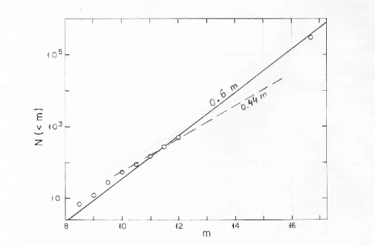
Figure 7: Hubble’s (1926) early result on the counts of bright galaxies. The single point at 16 mag was based on old data by Fath. The straight thick line has the slope of 0.6, which corresponds to the homogeneous cosmological model. The dashed line presents modern data from the LEDA database showing a slope of 0.44 in the interval $10^{m}\div 14^{m}$, corresponding to the fractal dimension $D=2.2$ (Teerikorpi 2004).

For the bright galaxies ($m<16$), the major shortcoming was the lack of data for the magnitude interval $12^{m}\div 16^{m}$ (see Fig. 7). We will discuss modern data in this interval in sect. 5.4.3.

Hubble was convinced that his data on bright galaxy counts already shows homogeneity. He considered that clusters of galaxies contain only a small fraction of all galaxies, and the true spatial distribution is quite homogeneous. Hubble’s conclusion had a strong impact on the theoretical cosmology, as expressed by Einstein in 1933: Hubble’s research has, furthermore, shown that these objects are distributed in space in a statistically uniform fashion, by which the schematic assumption of the theory of a uniform mean density receives experimental confirmation (cited by Peebles 1980). From this time on the picture of a uniform galaxy field with clusters as rare fluctuations became a paradigm of the homogeneous galaxy universe.

Later Hubble’s bright galaxy counts were used by Sandage, Tammann & Hardy (1972) to show the incompatibility with de Vaucouleurs’s hierarchical model with $\gamma=1.7$. For this $\gamma$ Eq.119 implies that $N(m)=0.26m+\mathrm{const}$, and this clearly differs from the value $0.6m$ from the counts by Hubble and Zwicky, available at that time. Hence they demonstrated that the hierarchical model with the fractal dimension $D=1.3$ cannot explain the galaxy number counts. Here we should emphasize that modern counts of bright galaxies in the range $10^{m}\div 14^{m}$ display a slope 0.44 which corresponds to $D=2.2$. This will be discussed in sect. 5.4.3.

4.3.2 Hubble’s deep galaxy counts.

Hubble (1934, 1936) extended the number counts up to the magnitude 21 in his massive galaxy count program on 1184 photographs on random positions in the sky. Each plate covered 0.25 deg². Now he did not confirm the $0.6m$ prediction at faint magnitudes, but instead the counts followed a $0.5m$ law. He did not abandon the hypothesis of homogeneity, but tried to explain this deflection as due to a redshift effect on galaxy magnitudes. He made a kind of K-correction and concluded that the $0.6m$ law may be obtained only in a non-expanding universe. In fact, to the end of his life (1953), Hubble regarded that the cosmological redshift may be caused by some other effect than expansion.

Sandage (1995) has analyzed Hubble’s counting programme and found three kinds of systematic errors which influenced Hubble’s calculations: 1) there were systematic errors in Hubble’s photographic magnitudes, making them increasingly too bright for fainter objects; 2) there was an error in the K-term as applied by Hubble; 3) when calculating the prediction of spatial volumes in the Friedmann model corresponding to different redshifts Hubble used an incorrect kind of distance. In the light of these problems, one may now see that Hubble’s old result on faint galaxies cannot be used as evidence neither for homogeneity nor non-expansion.

4.3.3 Variable dust extinction.

One argument against the reality of superclusters referred to our “dusty window” to extragalactic space. Because the early evidence for superclustering of galaxies came from the sky distribution, a natural objection was that one should take into account the variable light extinction in different directions of the sky, due to the cloudy dust distribution in the Milky Way.

Victor Ambartsumian developed the theory of a fluctuating Galactic extinction and applied it to the counts of extragalactic nebulae (Ambartsumian 1940; 1951). The paper by Neyman & Scott (1952) was devoted to their well-known two level clustering model. With references to Charlier (1922) and Ambartsumian (1951) they emphasize that there are in principle two approaches to galaxy clustering: 1) galaxies are really clustered in space; 2) the apparent clustering in the sky is caused by variable extinction due to interstellar dust clouds. Which factor dominates for clusters and superclusters? Later Holmberg (1975) and Fesenko (1975) further studied the role of inhomogeneous dust in the apparent galaxy clustering and concluded that the observed clustering is essentially modified by dust.

In the 1950s Zwicky (1955, 1957) proposed that also intergalactic dust, concentrated in clusters of galaxies, could cause extinction of background clusters. He studied the distribution of 921 clusters and found a deficit of clusters in regions around the Virgo, Coma and Ursa Major clusters of galaxies. This he interpreted as obscuration by intergalactic dust.

Also Karachentsev & Lipovetskii (1969) derived from counts of background clusters a positive mean value for the light extinction in clusters of galaxies. Their result was 0.2 magnitudes in the B band and they pointed out that there might have been selection effects influencing Zwicky’s own counts: e.g., seen behind nearby clusters it is more difficult for more distant clusters to fulfil the identification criteria. We note that Mattila (1978) measured the diffuse light in the Coma cluster and concluded that a part of it could be scattered light from intergalactic dust inside the cluster. Later he measured together with Stickel et al. (1998) the far-infrared emission of the dust in Coma. The emission was detected and it was calculated that it could cause only about 0.2 magnitudes or probably less of extinction.

Incidentally, Teerikorpi (2002) showed from the reddenings of quasars seen through galaxy halos (optical spectra of those quasars contain narrow absorption lines at much lower redshifts) that there is about 0.2 magnitudes of extinction per halo. Inside compact galaxy clusters and around the cores of rich clusters such as Coma the galaxy halos may almost overlap in projection and one might on this basis alone expect an extinction of the order of 0.1 mag.

It is interesting to note that Zwicky & Rudnicki (1963) concluded, taking into account the effects of interstellar and intergalactic absorption … that the results obtained confirm the assumption that the distribution of clusters of galaxies is uniform within a space whose indicative radius is of the order of $10^{9}$ pc. They inferred that clusters have different sizes up to a maximum 40 Mpc and there is no superclustering.

However, the argument from extinction loosed its power after massive measurements of galaxy redshifts led to the discovery of the very lumpy 3-d galaxy distribution. We note that the study of the galactic extinction continues to be relevant for many extragalactic subjects, including the fluctuations in the cosmic background radiation.

4.3.4 The classical “linearity” argument by Sandage, Tammann & Hardy.

De Vaucouleurs (1970) expected that mass density fluctuations cause deviations from the Hubble law and in particular in his hierarchical model the Hubble expansion rate should be reduced by gravitation inside the Local Supercluster. His PhD student Wertz (1971) developed a Newtonian expanding hierarchical model and calculated the predicted deflection from the linear Hubble law: the Hubble “constant” would increase with increasing distance within 20 Mpc from us.

By this time Sandage had collected redshifts for 82 first-ranked cluster galaxies, which splendidly allowed one to test the prediction of the hierarchical model. This test was performed by Sandage, Tammann & Hardy (1972) who confronted the observations with the calculations by Wertz (1971) and Haggerty & Wertz (1972) for the predicted deflection from the linear redshift–distance law. The result of the test was striking: the linear Hubble law with $H_{0}=$ constant was established at all tested scales, while the hierarchical model predicted so strong a deflection that one should not see any cosmological expansion at distances closer than 20 Mpc. Later observations only strengthened the argument from linearity: a smooth linear Hubble flow starts in the vicinity of the Local Group, already at 1.5 Mpc (Sandage & Tammann 1975; Sandage 1986, 1987).

Actually this test had a deeper meaning than being just a probe of the hierarchical distribution of luminous matter. It demonstrated a paradox: both empirical facts were true, i.e. the strongly inhomogeneous galaxy distribution in the local universe and the unperturbed linear Hubble law at the same scales. Sandage, Tammann & Hardy suggested two possible solutions for this paradox: 1) the mass density parameter could be very small, $\Omega_{0}\ll 1$, or 2) there could be an invisible uniform medium of high density. In both cases, the perturbations of the Hubble law would be tiny. In fact, from this post-classical cosmological test a whole new approach was developed, studying the properties of the cold very local Hubble flow (Chernin 2001; Baryshev, Chernin & Teerikorpi 2001; Macciò, Governato & Horellou 2004).

De Vaucouleurs (1972) did present evidence for a curved Hubble law in the local galaxy universe (the Hubble “constant” inferred from brightest group members strongly increased from small to large distances). Teerikorpi (1975a) studied the reality of such a behaviour using spiral galaxies with known van den Bergh’s luminosity classes $L_{c}$. These also showed a similar increase in $H$, but with a systematic shift depending on $L_{c}$. This gave the crucial hint that the phenomenon was not real, but was caused by a selection bias influencing distance measurements. In Teerikorpi (1975b, 1982) the bias was satisfactorily modelled both for luminosity classes with Gaussian luminosity functions and for the brightest group member criterion.

In Teerikorpi (1975a) the selection effect and its influence on the $V/R$ (“Hubble constant”) versus $V$ (radial velocity) diagram of luminosity classified was explained in a simple manner, which serves as an example how a strong bias may be caused by observational limits.

Assume that there is a limiting magnitude $m_{l}$ for the galaxy sample. Then in the $M--logR$ ($R=$ distance in Mpc) diagram only galaxies below the line $M=m_{l}-255\log R$ are available for mapping the kinematics of the local universe.

Now consider a class of galaxies with a true average absolute magnitude $M_{0}$, then the selection begins to affect distance determinations at least at the distance $R_{0}$ where $M_{0}=m_{l}-25-\log r_{0}$. It is easy to show that if $R$ is the erroneous distance calculated from $M_{0}$ at the real distance $R=V/H$, then the lower envelope of the points in the $V/R$ vs. $V$ diagram is defined by $V/R=V/R_{0}$ (when $R>R_{0}$). Note that the slope depends on $R_{0}$, i.e. on the $M_{0}$ of the luminosity class considered, when the limiting magnitude is constant.

4.3.5 Isotropy in a homogeneous universe.

Classically, from isotropy around one observer, together with the Copernican cosmological principle (“all points are alike”), one may infer the global homogeneity of the cosmological fluid (Walker 1944; for a simple geometric argument, see Weinberg 1977, p. 24). Before the 1970’s there were three major observational evidences for an isotropic matter distribution around us.

First, Hubble’s deep counts of faint galaxies (up to $m\approx 21$) did not show large differences in different directions of the sky, after correction for Galactic extinction. It is true that Shapley (1934) noted a considerable difference in the numbers of bright galaxies (up to $m_{pg}=13$) for the northern and southern galactic hemispheres. He also found that at $m\approx 18$ the galaxy numbers might vary across the sky by a factor of 2 on angular scales of $30^{o}$. However, these deviations were viewed as local fluctuations.

Second, the thousands of faint radio sources in the early catalogues (4C, Parkes, Molongolo, and others) were found to be uniformly distributed in the sky within statistical uncertainty (e.g. Holden 1966).

Third, already the first measurements by Conklin & Bracewell (1967) and Penzias, Schraml & Wilson (1969) of the cosmic background radiation found a remarkable isotropy at the level $\Delta T/T<10^{-3}$ on arc-minute scales.

These isotropies have generally been interpreted as strong evidence for homogeneity at scales larger than 1000 Mpc. Is it possible to have local isotropy within inhomogeneous distribution of matter? The answer is “yes” for self-similar statistically isotropic fractal structures. This question is also connected with a more general formulation of the Cosmological Principle, which we will discuss in the last section.

4.4 Results from angular galaxy catalogues

4.4.1 Main catalogues of galaxies and clusters.

In the 1950’s and 1960’s the first deep wide area catalogues of galaxies and galaxy clusters appeared, based on inspection of the monumental Palomar Sky Atlas photographic survey. This was the golden age of angular galaxy catalogues, from which the distribution of galaxies was investigated without distance information from the redshift. This important 2-d epoch in studies of galaxy clustering came to its end in the 1970’s when the data analysis of all available galaxy catalogues was completed.

The main catalogues were the Shapley–Ames (1932) Bright Galaxy Catalogue, Abell’s (1958) catalogue of rich galaxy clusters, the Reference Catalogue by de Vaucouleurs & de Vaucouleurs (1964), the Catalogue of Galaxies and Clusters of Galaxies by Zwicky et al. (1961-68), and the Lick counts in cells by Shane & Wirtanen (1967).

4.4.2 The angular correlation function analysis.

The main mathematical instrument for analyzing the above mentioned catalogues was the angular correlation function (CF) techniques, which is described in detail by Peebles (1980). The angular CF $w(\theta)$ is defined analogously to $\xi(r)$ as the excess probability relative to the Poisson expectation to find an object in the solid angle $\delta\Omega$ at the angular distance $\theta$ from randomly chosen objects in the sample:

$$\delta P=n\delta\Omega[1+w(\theta)].$$ (121)

Here $n$ is the mean surface density of objects in the sky.

A practical estimate of $w(\theta)$ for a sample of $N$ galaxies with known positions on the sky can be obtained by counting objects in rings of radius $\theta$ and width $\delta\theta$. The normalization condition is

$$N=n\int_{d\Omega_{s}}[1+w(\theta)]d\Omega,$$ (122)

where $\Omega_{s}$ is the solid angle of the survey. An important practical point is that if the 2-D projection of an inhomogeneous spatial distribution is close to homogeneous, then this method cannot detect this true inhomogeneity but regards it as a structureless Poisson distribution. We will see that this just happened with spatial structures having fractal dimension $D\geq 2$.

4.4.3 The relation between angular and spatial correlation functions.

The primary aim of the analysis of angular catalogues was to estimate the spatial correlation function $\xi(r)$ from the directly measured angular distribution of galaxies. The relation between $w(\theta)$ and $\xi(\theta)$ was first derived by Limber (1953), already in the context of galaxies (a useful review is by Fall 1979). For small angles $\theta$, Limber’s equation is:

$$w(\theta)=\int_{0}^{\infty}dxx^{4}\phi^{2}\frac{\int_{-\infty}^{\infty}dy\xi[(x^{2}\theta^{2}+y^{2})^{1/2}]}{[\int_{0}^{\infty}dxx^{2}\phi(x)]^{2}}$$ (123)

Here $\phi(x)$ is the sample selection function, defined as the fraction of galaxies per unit volume of space observable at a distance $x$ from Earth.

Eq.123 may be inverted analytically in order to obtain $\xi(r)$. However, a negative side is that this procedure requires differentiation of observed data which always contain some noise amplifying errors (Fall & Tremaine 1977).

An important particular case, which is useful in practice, is a power law solution of Eq.123. For the spatial correlation function in the form:

$$\xi(r)=Br^{-\gamma}=Br^{-(3-D)}$$ (124)

the corresponding angular correlation function is simply

$$w(\theta)=A\theta^{1-\gamma}=A\theta^{D-2},$$ (125)

where the constant $A$ comes from observations and the constant $B$ depends on $\gamma$ and the selection function $\phi$ (Fall 1979).

Caution: The power law solution (eq.125) exists only if

$$\gamma>1,\;\;\;\;D<2$$ (126)

As we already discussed in sec.2.4.5 according to theorem on fractals projection, this means that the method does not work for fractal structures with the fractal dimension $D\geq 2$. However, below we will see that the real galaxy distribution is characterized by the value of $D$ which is just within this critical range!

4.4.4 Hierarchical $D=1.2$ models for angular galaxy catalogues.

In their pioneering work Totsuji & Kihara (1969) derived from the angular data of the Lick galaxy counts a power law angular correlation function

$$w(\theta)=A\theta^{-0.8},$$ (127)

from which they finally obtained

$$\xi_{\mathrm{TK}}(r)=\left(\frac{4.7h_{100}^{-1}\mathrm{Mpc}}{r}\right)^{1.8}$$ (128)

In 1973 Peebles started an extensive programme analysing all angular galaxy and cluster catalogues, and asserted that all catalogues are characterized by almost the same power law with $\gamma=1.77$ and $r_{0}=5h^{-1}_{100}$ Mpc in scale intervals $0.1\div 10$ Mpc. A review of these results is given in Peebles (1980; 2001).

In fact, this was a rediscovery of de Vaucouleurs’s cosmological density–radius relation at small scales ($0.1\div 10$ Mpc). Totsuji & Kihara (1969) and Peebles (1974a) had for the first time found that the galaxy correlation function is a continuous power law with no peaks, as would be expected from preferred scales (case 2 in de Vaucouleurs 1970). Thus it naturally reflects the self-similarity of fractal structures. The exponent $\gamma=1.8$ corresponds to the fractal dimension $D=1.2$.

The new emerging picture of continuous hierarchy inspired the construction of protofractal models for the spatial galaxy distribution. Peebles (1974b) tried to find a general luminosity function of galaxies consistent with the power law hierarchy. Soneira & Peebles (1977, 1978) constructed a static hierarchical model of the galaxy universe. They used regular hierarchical model of Fournier’s type with 12 levels of galaxy pairs, so that $k_{N}=2$ and $k_{r}=1.76$ and according to eq.11 the fractal dimension $D=1.23$ or correlation exponent $\gamma=1.77$. The positions of galaxies are assigned according to the pair hierarchy, the luminosity function and apparent limiting magnitude were used to create a magnitude limited sample, and finally the galaxies were projected on the sky of an observer. Soneira & Peebles (1978) compared this binary hierarchy with Lick galaxy counts and concluded that even such a simple model reproduced well the angular correlation function of the observed galaxy distribution. Soneira & Peebles (1977) for Zwicky et al.(1961-68) Catalogue of Galaxies and Clusters of Galaxies, inferred that there is no evidence for a spatially uniform population of field galaxies. This confirmed the general tendency for galaxies to appear only in clusters.

4.4.5 Tallinn 1977 conference

A landmark event in the study of the galaxy distribution was the IAU Symposium N79 The large scale structure of the Universe held in Tallinn, Estonia, September 1977. Leading astronomers presented observational and theoretical works on galaxy clustering and it was the first wide discussion of all existing arguments for and against homogeneity at extragalactic scales.

Peebles (1978) presented a review of the angular correlation function analysis applied for all available angular galaxy catalogues. He emphasized that ”a small systematic error in the angular distribution can be translated into a very large error in the estimate of the spatial clustering” and that ”redshift data will allow us to avoid this problem”. Peebles argued that at distances $\leq 10$ Mpc the galaxy clustering is described by power law, but at larger scales the galaxy distribution became homogeneous. He referred the first time to the book by Mandelbrot (1977), where the idea of the fractal was extended to extragalactic scales.

Joeveer & Einasto (1978) presented an analysis of existing redshift data and concluded that the galaxy Universe has a cell structure with the mean diameter of voids about $50\,h_{100}^{-1}$ Mpc. The presence of large structures and holes of various sizes was also demonstrated at the symposium by de Vaucouleurs, Tully, Fisher, Abell, Tifft, Gregory, Kalinkov and others.

In his concluding remarks Longair (1978) noted that ”Everyone seemed to agree about the existence of superclusters … systems on scales $\sim 30-100$ Mpc.” However, when he refers to the results of angular correlation function analysis by Peebles’ group who derived a homogeneity scale at 10 Mpc, Longair asserted ”I am still a firm believer in the basic correctness of the covariance analysis”. Though the results presented by Kalinkov’s team about the third-order clustering point to the tendency of continuous galaxy clustering. Longair emphasized that ”One wonders whether their existence is consistent with the isotropy of the distribution of extragalactic radio sources and of the microwave background radiation”.

4.4.6 First evidence for the $D=2$ distribution

Though from the angular correlation function analysis the value of the fractal dimension $D\approx 1.2$ ($\gamma=1.8$) was derived, there were other evidences pointing at the fractal dimension $D\approx 2$. Historically, it is interesting that Lundmark (1927) made in effect the first observational estimate of the fractal dimension on the basis of Charlier’s model, noting that the second criterion is fulfilled, which corresponds to $D=2$.

Baryshev (1981) discussed some observational and theoretical arguments in favour of the fractal dimension $D\approx 2$. Using such observational cosmological data as: 1) the galaxy number counts $N(m)$ in a wide magnitude interval from $2^{m}$ up to $24^{m}$; 2) the virial mass density—radius relation $\rho_{vir}(R)$; 3) the peculiar velocity dispersion—radius relation $\sigma_{v}(R)$, he concluded that a hierarchical model of galaxy distribution with $\gamma=1$ (fractal dimension $D=2$) is consistent with the observations.

In that paper a new theoretical argument on a special property of fractals with the dimension $D=2$ was also presented. It comes from Bondi’s (1947) consideration of the global gravitational redshift part of the cosmological redshift. For a homogeneous matter distribution in the case of $z<<1$ the gravitational cosmological redshift is:

$$z_{grav}=\frac{\delta\phi(r)}{c^{2}}=\frac{1}{2}\frac{GM(r)}{c^{2}r}=\frac{1}{4}\Omega_{0}\left(\frac{r}{r_{H}}\right)^{2}$$ (129)

were $\delta\phi(r)=\phi(r)-\phi(0)$ is the gravitational potential difference between the observer and the source, $r_{H}=c/H_{0}$ is the Hubble radius.

It is very important that from the causality principle it follows that the source is in the centre of the matter ball with radius equal to the distance $r$ between the source and observer. Note that Zeldovich & Novikov (1984, p.97) and Peacock (1999, problem 3.4) put the observer to the centre of the ball and hence got the gravitational blueshift instead of Bondi’s gravitational redshift. However such a choice of the reference frame violates the causality in the process considered. Indeed, the event of emission of a photon by the source (which marks the centre of the ball) must precede the event of detection of the photon by an observer. The latter event marks the spherical edge where all potential observers are situated.

Generalizing eq.129 to the case of a fractal distribution where $M(r)\propto r^{D}$ one may derive the following relation for the gravitational part of the cosmological redshift within the fractal galaxy distribution:

$$z_{grav}=\frac{4\pi G\rho_{0}r_{0}^{2}}{c^{2}D(D-1)}\left(\frac{r}{r_{0}}\right)^{D-1}$$ (130)

where $\rho_{0},r_{0}$ are the density and radius of the zero level of the fractal structure (galaxies in our case).

For the fractal structure with $D=2$ the cosmological gravitational redshift is a linear function of distance:

$$z_{grav}(r)\;=\;\frac{2\pi G\rho_{0}r_{0}}{c^{2}}\;r\;=\;\frac{H_{g}}{c}\;r$$ (131)

where $H_{g}$ is the gravitational Hubble constant, which may be expressed as

$$H_{g}\;=\;2\pi\rho_{0}r_{0}\;\frac{G}{c}$$ (132)

For a structure with fractal dimension $D=2$ the constant $\beta=\rho_{0}r_{0}$ may be actually viewed as a new cosmological fundamental constant. If the value of the constant $\beta=1/2\pi$ g/cm² ( e.g. $\rho_{0}=5.2\times 10^{-24}$ g/cm³ and $r_{0}=10$kpc), then $H_{g}=68.6$ (km/s)/Mpc. So the linear Hubble law within the fractal structure with $D=2$ is possible, though it requires a very large amount of fractal-like distributed dark matter.

4.4.7 Why did angular catalogues lose the $D=2$ structure?

An explanation of why it is difficult to study a fractal structure with dimension $D\geq 2$ from angular distribution of galaxies was given by Baryshev (1981). If we model a part of the fractal as a spherical cluster of particles inside the radius $R$, then one can derive the surface distribution $F(\sigma)$ of the particles, projected on the sky, using the Abel equation

$$F(\sigma)=2\int_{\sigma}^{R}\rho(r)\frac{r\;dr}{\sqrt{r^{2}-\sigma^{2}}}\;$$ (133)

where $\sigma$ is the projected distance from the centre of the sphere.

For a power-law representation of a spherically symmetric fractal structure $\rho(r)=\rho_{0}(r_{0}/r)^{3-D}\propto r^{-\gamma}$ it is possible to obtain analytical solutions in closed form for fractal dimensions $D$ 3, 2, and 1. For a homogeneous ball ($D=3$, $\gamma=0$)

$$F(\sigma)=2\rho_{0}r_{0}\;\frac{R}{r_{0}}\sqrt{1-\frac{\sigma^{2}}{R^{2}}}\;.$$ (134)

For a structure with $D=2$ ($\gamma=1$) we get

$$F(\sigma)=2\rho_{0}r_{0}\;\left[\ln\left(1+\sqrt{1-\frac{\sigma^{2}}{R^{2}}}\right)+\ln\frac{R}{\sigma}\right]\;.$$ (135)

Finally, for $D=1$ ($\gamma=2$) the surface density will be

$$F(\sigma)=2\rho_{0}r_{0}\;\frac{r_{0}}{\sigma}\arccos\frac{\sigma}{R}\;.$$ (136)

Hence for the values of $\sigma<<R$ the surface density behaves approximately as

$$F(\sigma)\sim\mathrm{const}\,,\,\,\,\,\,\mathrm{for}\,\,\,\,D=3\,,$$ (137)

$$F(\sigma)\sim\ln\sigma\,,\,\,\,\,\,\mathrm{for}\,\,\,D=2\,,$$ (138)

$$F(\sigma)\sim\sigma^{-1}\,,\,\,\,\,\,\mathrm{for}\,\,\,D=1\,.$$ (139)

Both for $D=2$ and $D=3$ the surface density varies slightly, which means that the projected distribution appears on the sky with a homogeneous surface density.

This derivation demonstrates that the angular correlation function analysis becomes inefficient for structures with the fractal dimension close to or larger than 2, because the information on the 3-d structures with $D\geq 2$ is lost as the projected on the sky 2-d distribution approaches homogeneity. As we already emphasized this result is a consequence of the general theorem on fractal projections (sect. 2.4.5) with its critical dimension $D_{pr}=2$.

5 Debate on fractality: the epoch of spatial maps

During the 1980s several galaxy redshift catalogues (see Table 1) became available for the 3-d analysis of spatial maps. This brought into light unexpected news about different behaviour of the $\xi$-correlation function for different samples of galaxies and clusters of galaxies. It was then realized within some research teams that the fractal galaxy structure can naturally explain the peculiarities of the measured $\xi$-function, and also that the appropriate mathematical tool for the analysis of fractals is the method of $\Gamma$-function. Since then the fractal approach has given rise to new fruitful directions for observational and theoretical studies.

5.1 The fractal breakthrough in the 1980s.

After the concept of the fractal entered the scene of the LSS of the Universe, the cosmological community as if divided into two parts. One continued to use the $\xi$-function method, which led to the conclusion about the absence of a galaxy ”fair sample”. The second, smaller, group started to apply the fractal approach based on the $\Gamma$-function method, and they obtained concordant results from different galaxy samples.

5.1.1 Davis & Peebles $\xi$-function analysis of the CfA sample of galaxies

The paper by Davis & Peebles (1983; hereafter DP83) was in many ways classical. It presented the first systematic analysis of the CfA data by the $\xi$ correlation function method. The CfA catalogue was the result of the first large redshift survey of the Harvard-Smithsonian Center for Astrophysics (CfA), which was complete to $m_{B}=14.5$ in the sky regions $(\delta>0\,,\,\,b>40^{o})$ and $(\delta\geq-2.5^{o}\,,\,\,b<-30^{o})$). It contained 2400 galaxies with redshifts.

DP83 extracted a volume-limited subsample with $M_{B}<-18.5+5\log h_{100}$ which contained 1230 galaxies in the Northern zone and 273 galaxies in the Southern zone.

In DP83 used the concepts of redshift-space and real-space correlation functions were utilized, developed by Peebles (1980). They also took into account the peculiar velocities, using the method, which we considered in sect. 3.2.5. They found the rms line of sight peculiar velocity distribution

$$\sigma_{v}(r)=340\pm 40(\frac{r}{\mathrm{Mpc}\,h_{100}^{-1}})^{0.13\pm 0.04}\,\mathrm{km/s}$$ (140)

From the 3-d rms peculiar velocity the “cosmic energy equation” gives (Peebles 1980; Eq.74.9):

$$<v_{\mathrm{pec}}>^{1/2}\approx 850\Omega_{0}^{1/2}\mathrm{kms}^{-1}$$ (141)

which may be used to estimate the density parameter $\Omega_{0}$. For CfA DP83 obtained $\Omega_{0}\approx 0.2$ for the component of matter clustered with the galaxy distribution on scales $r<1h_{100}^{-1}$ Mpc.

DP83 suggested the $\xi$-function estimator which later came to be called standard. The calculation of data–random pairs was introduced for a correction of the edge effect and to reduce the shot noise on small scales.

The main conclusion of DP83 was that the real-space two-point correlation function after the projection has a power-law form $\xi\propto r^{-\gamma}$

$$\xi_{\mathrm{DP}}(r)=\left(\frac{5.4h_{100}^{-1}\,\mathrm{Mpc}}{r}\right)^{1.74}\,,$$ (142)

in the surprisingly wide interval of scales

$$10\,h_{100}^{-1}\,\mathrm{kpc}\,<\,r\,<\,10\,h_{100}^{-1}\,\mathrm{Mpc}\,.$$ (143)

Together with estimated errors the $\xi$-function parameters were $r_{0}=5.4\pm 0.3\,h_{100}^{-1}\,\mathrm{Mpc}$ and $\gamma=1.74\pm 0.04$. It is important that for scales $r>10\,h_{100}^{-1}\,\mathrm{Mpc}$ the $\xi$-function drops, changes sign, and starts to oscillate near the zero-level. From what we considered in sect.3.2.3., this is exactly what is expected for the $\xi$-function estimator.

After this pioneering work, the values of the unit scale $r_{0}\approx 5\,h_{100}^{-1}$ Mpc (defined as $\xi(r_{0})=1$) and the correlation exponent $\gamma\approx 1.8$ have been generally considered as standard cosmological numbers (see Peebles (2001) in the conference “Historical Developments of Modern Cosmology”).

As we discussed in sec.3 the $\xi$-function method actually gives a distorted value for the intrinsic power-law exponent $\gamma_{true}$ of a fractal structure, hence these results contain systematic errors. However at that time it seemed that the first 3-d map gave results which are consistent with analysis of angular catalogues and that the galaxy distribution becomes homogeneous on scales larger than $20\,h_{100}^{-1}$ Mpc .

5.1.2 The puzzling behaviour of the $\xi$-function

When the first redshift surveys were studied by means of the $\xi$-function method, a new unexpected problem appeared. The characteristic length $r_{0}$ was found to be dependent on certain parameters of the samples, such as the depth of a survey, the type and luminosity of galaxies and clusters, and the mean separation between the objects in the sample.

Contrary to the expectation that “the spatial correlation function of galaxies is quite small for separations greater than about $20h_{100}^{-1}$ Mpc”, it was found by Bahcall & Soneira 1983 and Klypin & Kopylov 1983 that the characteristic length $r_{0}$ (and hence the amplitude of the $\xi$-function) become quite large for clusters of galaxies.

Bahcall & Soneira (1983) calculated the redshift-space $\xi$-function for a complete sample of $N=104$ Abell clusters with the distance class ($\leq 4$), and obtained the following estimates of its parameters:

$$r_{0}^{cl}\approx 25\,h_{100}^{-1}\mathrm{Mpc}\,,\,\,\,\,\gamma^{cl}\approx 1.8$$ (144)

Klypin & Kopylov (1983) studied another sample of Abell clusters with $z<0.08$ and $\|b\|\geq 30^{o}$. Their catalogue contained $N=158$ rich clusters of galaxies including redshifts measured with the 6-meter telescope of the Special Astrophysical Observatory of USSR Academy of Sciences. The redshift-space $\xi$-function for the sample had the following parameters

$$r_{0}^{cl}\approx 25\,h_{100}^{-1}\mathrm{Mpc}\,,\,\,\,\,\gamma^{cl}\approx 1.6$$ (145)

These results revealed a significant discripancy between the unit scales $r_{0}$ for galaxies (5 Mpc) and for clusters (25 Mpc).

Moreover, when the $\xi$-function was calculated for superclusters of galaxies (Bahcall & Burgett 1986; Lebedev & Lebedeva 1988), even larger scale were found:

$$r_{0}^{cl}\approx 60\,h_{100}^{-1}\mathrm{Mpc}\,,\,\,\,\,\gamma^{cl}\approx 1.8$$ (146)

According to these data the correlation length $r_{0}$ increases from 5 to 60 $h_{100}^{-1}$Mpc when one considers increasingly massive objects in the universe.

An important property of this new effect was also found by Einasto, Klypin & Saar (1986) who studied the behaviour of $r_{0}$ within galaxy and cluster samples having increasing volumes. They used a cubic geometry for galaxy samples with the edge size $l=R_{s}$ (which is the depth of a survey) and found an approximately linear relation beween the unit scale and the depth of the sample:

$$r_{0}\propto R_{s}\,.$$ (147)

In the framework of Gaussian density fluctuations on a homogeneous background this behaviour of $\xi$-functions is an enigmatic fact, and to explain it several possibilities were discussed (Kaiser 1984; Bardin et al. 1986; Davis et al. 1988; Bahcall 1988).

The most popular one is Kaiser’s idea of biased galaxy formation, based on a possible relation between the correlation functions for galaxy clusters and for the underlying mass density field. Here clusters are regarded as rare high density spots in the density field, so that one might expect

$$\xi_{\mathrm{clusters}}=b\xi_{\mathrm{density}}(r)\,,$$ (148)

where $b$ is the bias factor which is about 10 if $\xi_{\mathrm{density}}=\xi_{\mathrm{galaxies}}$. This means that galaxies in clusters are formed from rare peaks above some global threshold in the primordial density field. However, the validity of this explanation in the case of Gaussian density fields was recently critisized by Gabrielli, Sylos Labini & Durrer (2000). They demonstrated that the increasing sparseness of peaks over the threshold in Gaussian random fields does not explain the observed increase of the amplitude of the correlation function $\xi(r)$.

Other alternative possibilities, like local inhomogeneities, corrections for Galactic extinction, and luminosity segregation (Davis et al. 1988), look surprising and demand careful future studies with much larger galaxy samples.

5.1.3 Pietronero’s solution of the mystery of $r_{0}$

A radically new interpretation of the observed $\xi$-function behaviour was found by Pietronero (1987) within the fractal approach to galaxy distribution. In this classical paper he introduced the $\Gamma$-function method for the 3-d galaxy map analysis and derived the relation between the $\Gamma$ and $\xi$ functions which we considered in sec.3.4.

For a spherical (or cubic) galaxy sample with the depth $R_{s}$ and a fixed luminosity of galaxies Pietronero (1987) obtained for the characteristic scale $r_{0}$, defined as $\xi(r_{0})=1$, the relation

$$r_{0}=(\frac{3-\gamma}{6})^{1/\gamma}R_{s}$$ (149)

Hence within a fractal model one expects a linear dependence of $r_{0}$ on $R_{s}$. An important consequence of eq.149 is that the increasing amplitude of $\xi$-function and the corresponding increase of $r_{0}$ for samples with larger $R_{s}$ is not due to a larger correlation length, but is simply an artificial effect caused by the definition of the reduced correlation function. In Fig.3 of Pietronero (1987) it was clearly demonstrated that the cause of the increasing amplitude of $\xi$-function is the increasing depth of a sample within the fractal structure.

If the picture of the universal fractal galaxy distribution is true, then the method of $\Gamma$-function, appropriate for fractal structures, will reveal a power-law behaviour for future still deeper galaxy samples. The requirement of spherical geometry for a sample is the most important restriction for deep galaxy surveys.

The first analysis of the CfA galaxy redshift catalogue by means of the $\Gamma$-function method was performed by Coleman, Pietronero & Sanders (1988). They found a power-law $\Gamma$-function with $\gamma=1.5\pm 0.2$, for VL samples with $N_{gal}=226$ and 442. The fractal behaviour was detected on the interval of scales from $1\,h_{100}^{-1}$ Mpc up to $20\,h_{100}^{-1}$ Mpc without any characteristic scale, contrary to the homogeneity scale $r_{0}=5\,h_{100}^{-1}$ Mpc derived by the $\xi$-function method.

5.1.4 Cellular fractal structure of the Universe

Just a few months after Pietronero’s (1987) paper, the fractal interpretation of the ”correlation length” versus depth was applied to redshift data by Calzetti, Einasto, Giavalisco, Ruffini, & Saar (1987). They confirmed the linear relation between $r_{0}$ and $R_{s}$, when the depth changed from $5\,h_{100}^{-1}$ Mpc up to $50\,h_{100}^{-1}$ Mpc.

Then in a series of papers of a team led by Ruffini a cellular model of the Friedmann universe was developed, where within cells with sizes of about 100 Mpc the distribution of galaxies has the fractal dimension $D\approx 1.2$, and on larger scales the universe becomes homogeneous (Ruffini, Song, & Taraglio 1988; Calzetti, Giavalisco & Ruffini 1988; Calzetti, Giavalisco & Ruffini 1989) . Their main conclusion was that de Vaucouleurs’s density law may be reconciled with the homogeneous Friedmann model if there is a maximum scale of fractality.

The Ruffini at al. model is based on the assumption that there are massive dark matter particles, called ”inos”, which obey Fermi statistics and are responsible for the initial density fluctuations of the cellular structure formation. The characteristic value of the ”ino” rest-mass-energy is $0.4\div 10$ eV, and the corresponding density parameter is $\Omega_{inos}=(0.4\div 1)$. An expected value of the size of the fractal cell is about 100 Mpc, which is determined by the Jeans length at the epoch when ”inos” decoupled from matter. The angular scale of the corresponding CMBR fluctuations is about 1 degree.

However, they used the lower value of the fractal dimension $D\approx 1.2$ derived from the $\xi$-function analysis, which is actually a distorted value of the true fractal dimension $D\approx 2$ obtained by means of the appropriate $\Gamma$-function method. It would be interesting to reconsider their model for $D\approx 2$.

5.1.5 The multifractal confusion from the $D_{2}=1.2$ estimation using the $\xi$-function method

Almost at the same time another group of astronomers started to apply the fractal approach for a description of the galaxy distribution. However, now we may see that their work was affected by a distorted estimate of the correlation fractal dimension from the $\xi$-function method.

Jones, Martinez, Saar & Einasto (1988) and Martinez & Jones (1990) noted that when they applied the methods of box-counting and minimal spanning tree for determining the Hausdorf dimension $D_{H}$ of the CfA redshift survey, they obtained the value $D_{H}=2.1\pm 0.1$. However, from the $\xi$-function for the same galaxy catalogue they concluded that the correlation dimension differs from this value, $D_{2}=1.2$, hence ”the Universe is not a simple fractal. It is a more complex structure, a multifractal” (Martinez & Jones 1990). An analogous conclusion was made by Klypin et al. (1989) and Balian & Schaeffer (1989).

Here we have an example of how inappropriate methods of data analysis may lead to erroneous theoretical conclusions. Indeed, as we discussed in sec.3.4 the estimation of the fractal dimension from the $\xi$ correlation function as $D_{2}=3-\gamma_{\xi}$ at scales close to $r_{0}$ gives a distorted value for the true codimension $\gamma$ because there $\gamma_{\xi}(r=r_{0})\approx 2\gamma$. Hence to calculate the true value of the correlation dimension from the slope of the $\xi$-function near $r=r_{0}$ one should take into account this distorsion, so $D_{2}=3-\gamma=3-(\gamma_{\xi}(r=r_{0})/2)=2.1$ for the observed slope $\gamma_{\xi}(r=r_{0})=1.8$.

Therefore one may conclude that actually $D_{2}\approx D_{H}$, i.e. the correlation dimension is consistent with the Hausdorf dimension for the CfA catalogue and there is no need for multifractality based on a difference between these dimensions. Modern results of $\Gamma$-function analysis for CfA, 2dF,SDSS and other galaxy redshift surveys confirm the value for the correlation dimension $D_{2}\approx 2$, and hence eliminate the above confusion on multifractality (see sec.5.3).

5.1.6 Balatonfured 1987 conference and observational evidence for very large structures

Parallel with developments of statistical methods for the analysis of fractal galaxy distribution in the 1980s, new observational evidence appeared supporting the existence of galaxy structures with sizes much larger than the characteristic homogeneity scale $r_{0}$ derived from the $\xi$-function analysis.

The results of a decade of intensive research after the Tallinn’77 conference were discussed at the 130th IAU Symposium ”Large Scale Structures of the Universe”, held in Balatonfured, Hungary 1987. It happened that this symposium became the last one on cosmology for Yakov Zeldovich (1914–1987) and for one of his talented pupils Victorij Shvartsman (1945–1987) who had just started to investigate the large scale structure of the Universe at the Special Astrophysical Observatory (SAO) of the USSR Academy of Sciences.

At the Balatonfured’87 conference new observational data on the reality of galaxy structures with sizes of about 100 Mpc were presented. Huchra, Geller, de Lapparent & Burg (1988) discussed an extension of the CfA redshift survey, which for several years was the main test bench for different statistical methods of the galaxy distribution analysis. They concluded that empty regions (voids) and filaments are common in the observed galaxy distribution, and the sizes of voids achieve $50\,h_{100}^{-1}$ Mpc, which is much larger than the characteristic $\xi$-function scale $r_{0}\approx 5\,h_{100}^{-1}$ Mpc.

Karachentsev & Kopylov (1988) reported the results of a spectral survey of 245 galaxies with $m_{B}\leq 17.5$ in a narrow strip which passed through the Coma cluster. They confirmed a bubble-like type of structure within the Coma supercluster and estimated the parameters of the $\xi$ correlation function: $r_{0}=22\,h_{100}^{-1}$ Mpc and $\gamma=1.5$. The average size of 14 voids was estimated to be about $25\,h_{100}^{-1}$ Mpc.

The most prominent structures were discovered by studies of rich galaxy clusters. Tully (1986, 1987) analyzed the distribution of 47 Abell clusters within a region up to $z=0.1c$ and found a flat structure having a size of about $300\,h_{100}^{-1}$ Mpc. This is called the Pisces–Cetus Supercluster Complex.

Similar results for an even deeper survey of galaxy clusters were obtained by Kopylov, Kuznetsov, Fetisova & Shvartsman (1988). They presented the first result of the program ”The Northern Cone of Metagalaxy” which included measurements of redshifts up to $z=0.28$ for 58 rich compact clusters of galaxies inside the cone with $b^{II}>60^{o}$. From these data they made a preliminary statement on the existence of inhomogeneities in the distribution of galaxies on scales up to $500\,h_{100}^{-1}$ Mpc.

In the Summary of the conference made by Peebles (1988) one may read: There is considerable evidence of structure on scales $\geq$ 50 $h^{-1}$ Mpc, but I think it is fair to repeat the old questions: could this be an artifact of errors in the catalogues? Could the eye be picking patterns out of noise? If the answers were definitely ”no” it would be very damaging for scale invariant cold dark matter. We all will be following the debate with great interest.

It took one more decade of hard observational work to disclose the reality of such super-large structures in galaxy distribution, but the debate is still going on how damaging it actually is for the CDM models.

5.2 Further steps in the debate

After the new idea of fractality entered the studies of large-scale galaxy distribution there was a period of strong opposition from those who used conventional methods of analysis. Fortunately in science the collision of ideas is actually needed for a deeper understanding of the universe. This was also the case with the fractal galaxy distribution, which gave an alternative to homogeneous matter distribution in the Universe.

5.2.1 Princeton “Dialogues’96”: Davis’s evidence for homogeneity at scales larger $20\,h^{-1}_{100}\,{\rm\mbox{Mpc}}$

In 1996 an international astronomical meeting under the intriguing title ”Critical Dialogues in Cosmology” was held in Princeton. Remarkably the first subject which opened the conference was the dialogue between Marc Davis and Luciano Pietronero on the homogeneity of the galaxy distribution.

Davis (1997) presented the position ”that there is overwhelming evidence for large scale homogeneity on scales in excess of approximately $50\,h^{-1}_{100}\,{\rm\mbox{Mpc}}$, with a fractal distribution of matter on smaller scales”. He emphasized that the observed correlation function $\xi(r)$ is well characterized by a power law, $\xi(r)\approx(r/r_{0})^{-\gamma}$, with $r_{0}\approx 5\,h^{-1}_{100}\,{\rm\mbox{Mpc}}$ and $\gamma=1.8$. Hence the fractal dimension at scales $r<r_{0}$ is $D=1.2$.

Davis’ arguments for homogeneity were:

• D1. Isotropy of the CMBR, X-ray and radio source counts.

• D2. Observed counts of galaxies for magnitude range $14<m<18$ have slope $0.6m$.

• D3. The observed angular correlation function $w(\theta)$ is reliable for recovery of spatial correlation function $\xi(r)$.

• D4. Analysis of four VL samples from 1.2 Jy IRAS redshift survey give for $\xi(r)$ standard values of $\gamma$ and $r_{0}$ when the volume limiting radius is increased from $60\,h^{-1}_{100}\,{\rm\mbox{Mpc}}$ up to $120\,h^{-1}_{100}\,{\rm\mbox{Mpc}}$.

• D5. ”The end of greatness” seen from the LCRS redshift survey.

• D6. Ly-$\alpha$ clouds detected in qso absorption spectra appear to be very nearly uniformly distributed in space.

After discussing his arguments Davis concluded: ”The measured two-point galaxy correlation function $\xi(r)$ is a power law over three decades of scale and approximates fractal behavior from scales of $0.01\,h^{-1}_{100}\,{\rm\mbox{Mpc}}<r<10\,h^{-1}_{100}\,{\rm\mbox{Mpc}}$, but on scales larger than $\approx 20\,h^{-1}_{100}\,{\rm\mbox{Mpc}}$, the fractal structure terminates, the rms fluctuation amplitude falls below unity, and the Universe approaches homogeneity, as necessary to make sense of a FRW universe.”

5.2.2 Princeton “Dialogues’96”: Pietronero’s arguments for fractality

Pietronero presented the statistical method ($\Gamma$-function analysis) which is relevant for study the fractal structures, compared it with the $\xi$-function method, and demonstrated the first results of application of both methods to the available redshift catalogues (Pietronero, Montuori, Sylos Labini 1997).

Pietronero’s main arguments for the fractality of the galaxy distribution were:

• P1. The projection effect of a spatial fractal structure may lead to the observed isotropy on the sky for the angular distribution of astrophysical sources.

• P2. A small number effect in the counts of bright galaxies may lead to observed $0.6m$-law even for fractal distribution.

• P3. The method of $\xi$ correlation function gives artificially distorted values both for the fractal dimension $D$ and for the homogeneity scale $r_{hom}$.

• P4. The method of $\Gamma$-function (conditional density) is appropriate for estimation of the true value of the fractal dimension $D$ and for detection of the crossover to homogeneity.

• P5. The $\Gamma$-function analysis of available 3-d galaxy catalogues, CfA, PP, IRAS, LEDA, LCRS, ESP, gives the value $D=2.0\pm 0.2$ for the fractal dimension at scales up to the radius $R_{max}^{sph}$ of the largest sphere that can be contained in the sample.

• P6. The homogeneity scale is not yet reached in existing galaxy catalogues and may be as large as $150\,h^{-1}_{100}\,{\rm\mbox{Mpc}}$ (LEDA result) and even as $1000\,h^{-1}_{100}\,{\rm\mbox{Mpc}}$ (number counts of ESP redshift galaxy survey).

Both sides of the discussion agreed that the galaxy distribution is a fractal structure at least within scales $0.1\div 10\,h^{-1}_{100}\,{\rm\mbox{Mpc}}$. But they disagreed about the values of the fractal dimension (Davis for $D\approx 1.2$ and Pietronero for $D\approx 2$) and about the value of the homogeneity scale (Davis for $R_{hom}\approx 20\,h^{-1}_{100}\,{\rm\mbox{Mpc}}$ and Pietronero for $R_{hom}\geq 150\,h^{-1}_{100}\,{\rm\mbox{Mpc}}$). Pietronero also emphasized that possible existence of uniformly distributed dark matter may reconcile Friedmann homogeneous model with observed visible fractal structure.

5.2.3 The problem of sky projection of fractals

One of the strongest argument for the value of fractal dimension $D=1.2$ and the homogeneity of galaxy distribution in space at scales larger than $r_{0}=5\,h^{-1}_{100}\,{\rm\mbox{Mpc}}$ was the claim that the analysis of galaxy angular catalogues led to just such values for the parameters of the angular correlation function.

Indeed, starting with Totsuji & Kihara (1969) in all angular galaxy gatalogues the analysts found the universal behaviour of the angular correlation function $\xi_{ang}(\theta)\propto\theta^{-\alpha}$ with $\alpha\approx 0.8$. For scales $r<r_{0}$ this would correspond to the fractal dimension $D$ in 3-d space $D=2-\alpha\approx 1.2$. As this is less than 2, then according to the fractal projection theorem (sect.2.4.5) one can estimate the true fractal dimension from the galaxy distribution projected on the sky.

Unfortunately, this logic has a flaw. Indeed, if the real spatial galaxy distribution is a fractal structure with $D\geq 2$ we would not be able to detect it from observations of the angular distribution of galaxies. This is because according to the fractal projection theorem the projected distribution imitates a homogeneous surface density. Consequently, 3-d maps are necessarily required to discover fractal structures with $D\geq 2$.

It is an intriguing fact that the fractal analysis of modern extensive 3-d galaxy maps has revealed $D\approx 2.2$, just putting the fractal dimension into that critical interval.

A decade after the first warning on the possible “conspiracy” of structures with $D\geq 2$ by Baryshev (1981), detailed studies started to appear on the complex problem of angular projections (Dogterom $ Pietronero 1991; Coleman & Pietronero 1992; Durer et al. 1997; Montuori & Sylos Labini 1997; Eckmann et al. 2003).

The method of angular $\Gamma$-function. The best demonstration of the consistency of the observed angular and spatial fractal structures with $D\approx 2$ was given by Montuori & Sylos Labini (1997). They studied 3-d maps together with the corresponding angular distributions from several redshift catalogues: CfA1, SSRS1, Perseus-Pisces, APM bright galaxies, and Zwicky galaxies. For an undistorted estimation of the correlation exponent in angular data they used the conditional surface density $\Gamma_{\mathrm{ang}}$

$$\Gamma_{\mathrm{ang}}(\theta)=\frac{1}{S(\theta)}\frac{dN(\theta)}{d\theta}=\frac{B_{\mathrm{ang}}D}{2\pi}\theta^{-\alpha}$$ (150)

where $S(\theta)d\theta$ is the solid angle element ($S(\theta)\approx 2\pi\theta$ approximated for small angles $\theta\ll 1$), $N(\theta)=B_{\mathrm{ang}}\theta^{D}$ is the number of galaxies in the “polar cap” with the radius $\theta$, $D$ is the fractal dimension of the 3-d structure, which with the condition $0\leq D<2$ coincides with the fractal dimension $D_{\mathrm{pr}}$ of the projected structure according to the fractal projection theorem (see sect.2.4.5). $\alpha$ is the angular correlation exponent related to the fractal dimension $D$ as

$$\alpha=2-D=\gamma-1$$ (151)

The last equality follows from the relation between the spatial and angular $\Gamma$-functions. The first one is the usual 3-d $\Gamma$-function $\Gamma(r)\propto r^{-\gamma}$ with $\gamma=3-D$, and the second one is the angular $\Gamma$-function $\Gamma_{\mathrm{ang}}\propto\theta^{-\alpha}$ with $\alpha=2-D$.

The result of this angular and spatial $\Gamma$-function analysis demonstrated very clearly that the fractal dimension of the observed 3-d structure is

$$D=1.9\pm 0.1$$ (152)

which was derived from independent analyses of the angular catalogues and 3-d maps. The angular correlation exponent was $\alpha=0.1\pm 0.1$ and the spatial correlation exponent was $\gamma=1.1\pm 0.1$ for all above mentioned catalogues.

The most amazing fact is that the previously derived “universal” value of the angular correlation exponent $\alpha_{w}=0.8$ is an artificial effect caused by the method of the angular $\xi$-correlation function $w(\theta)$ (sect. 4.4). This reduced correlation function gives systematically distorted values of the true correlation exponent due to the normalization condition.

We see here again that the whole story of how to find the true correlation exponent revolves around the difference between the power-law behaviour of the complete correlation function and the corresponding non-power-law reduced correlation function. This happens both for angular and spatial distributions.

5.2.4 Modern research topics related to large scale fractality

The debate on the nature of the large-scale structure of the visible matter in the Universe inspired many astronomers and physicists to study different aspects of the fractality galaxy distribution. The spectrum of subjects is very wide and shows that the principal questions, already raised by Einstein(1917, 1922) and Selety(1922, 1923) on the properties of hierarchical cosmological models, now are under careful investigation and actually they generate new branches of cosmological physics.

In Table 3 we present a list of main reseach topics together with corresponding references which demonstrate the variety of cosmological aspects touched by the fractality of the large scale structure of the Universe. We shall discuss some results of the studies in the sec.6 of the review.

Table 3: Main research topics related to large scale fractality.

Subject	References
conditional density	Pietronero 1987; Coleman, Pietronero 1992; Gabrielli et al. 2004
new methods of data analysis	Bharadwaj et al. 1999; Best 2000; Martinez, Saar 2002;
2-point conditional column density	Baryshev, Bukhmastova 2004; Vasiliev 2004
fractal dimension	Coleman et al. 1988; Klypin et al. 1989; Lemson, Sanders 1991;
of galaxy distribution	Jones et al. 1988; Martinez, Jones 1990; Jones et al. 1992;
scales of fractality	Sylos Labini, Montuori, Pietronero 1998
mass-radius relation for all scales	Sidharth 2000; Teerikorpi 2001; Rost 2004
local radial galaxy distribution	Sandage 1995; Teerikorpi et al. 1998; Teerikorpi 2004
number counts, normalization	Baryshev 1981; Joyce, Sylos Labini 2001; Courtois et al. 2004
luminosity function, multifractals	Sylos Labini, Pietronero 1996
dependence of correlation function	Einasto et al. 1986; Calzetti et al. 1987; Davis et al. 1988
on depth, luminosity	Norberg et al. 2001, 2002
type of object	Klypin, Kopylov 1983; Bahcall 1988; Bahcall et al. 2003
peculiar velocities	Zehavi et al. 2002, 2004; Hawkins et al. 2003
local fractal dimension	Tikhonov, Makarov, Kopylov 2001; Tikhonov, Makarov 2003
linearity and coldness of	Sandage et al.1972; Sandage 1986, 1987; Karachentsev et al.1996
the local Hubble flow	Ekholm et al. 2001; Karachentsev et al. 2003a,b; Whiting 2002
protofractal (hierarchical) models	Wertz 1971; Wesson 1975; Soneira, Peebles 1977, 1978
relativistic fractal models	Bonnor 1972; Ruffini et al. 1988; Ribeiro 1993; Gromov et al 2001
cosmological tests, fractal universe	Fang et al 1991; Baryshev et al. 1994; Joyce et al. 2000
cosmological gravitational redshift	de Sitter 1917; Bondi 1947; Baryshev 1981, 1994
local tests of cosmological vacuum	Chernin 2001; Baryshev et al. 2001; Axenides et al. 2002
and dark energy within fractals	Chernin et al. 2004; Maccio et al. 2004
statistical mechanics of	Perdang 1990; de Vega, Sanchez, Combes 1996, 1998
self-gravitating fractal gas, $D=2$	Combes 1998; Huber & Pfenniger 2001;
N-body simulation,	Governato et al. 1997; Moore et al. 2001
local structure	Klypin et al. 2003; Maccio et al. 2004
initial conditions and discreteness	Bottaccio et al. 2002; Baertschiger et al 2002; 2004
stability, velocity, force	Gabrielli, Sylos Labini, Joyce, Pietronero 2004
origin and evolution of	Haggerty 1971; Peebles 1974a; Alfven 1982; Lerner 1986
large scale fractals	Ostriker et al.1981; Pietronero et al.1986; Schulman et al.1986
	Szalay, Schramm 1985; Maddox 1987; Luo, Schramm 1992
cosmological principle	Mandelbrot 1975, 1977; Pietronero, Sylos Labini 1995;
and fractality,	Rudnicki 1995; Wu, Lahav, Rees 1999; Baryshev,Teerikorpi 2002
isotropy and homogeneity	Mandelbrot 1989; Sylos Labini 1994

5.3 Recent results from the $\xi$ and $\Gamma$ functions analyses

As we discussed above the crucial parameters for correlation analysis of a galaxy distribution are: 1) the average separation distance between nearest neighbour galaxies $R_{sep}$, 2) the radius of the maximum sphere completely contained in a sample $R_{max}^{sph}$, 3) the absolute magnitude interval $\triangle M_{i}$ of selected galaxies, and 3) the number of galaxies in a volume limited sample $N_{gal}$. To extract reliable information on the correlation exponent and a homogeneity scale one shoud be aware of the restrictions of the method used for the estimation. We shall see that within the common interval of applicability both $\xi$ and $\Gamma$ functions analyses give compatable results.

5.3.1 The redshift space $\xi$- and $\Gamma$- functions

$\xi$- and $\Gamma$-function analysis of the 2dF data. The final release of 2dF galaxy redshift survey (Colless et al. 2001; 2003) opens a new possibility for performing different kinds of statistical analysis of large samples of galaxies.

The 2dF galaxy redshift survey contains about 220 000 galaxies in two (NGP and SGP) narrow slices of about $90^{o}\times 15^{o}$ (SGP) and $75^{o}\times 10^{o}$ (NGP) complete up to $b_{j}=19.5$, with the effective reshift $z_{s}\approx 0.15$, and the effective absolute magnitude $M_{s}-5\,log\,h_{100}\approx-20.0$, corresponding to the luminosity $L_{s}\approx 1.4L^{*}$ (Norberg et al. 2002).

These data were analyzed using the $\xi$-function method of the reduced correlation function by Hawkins et al. (2003). The redshift-space correlation function was approximated by two different power-law forms (their figs.5,6,7), first, as

$$\xi_{z}(s)=\left(\frac{13\,h_{100}^{-1}\mathrm{Mpc}}{s}\right)^{0.75}\,,$$ (153)

for the interval of scales $0.1<s<3\,h_{100}^{-1}$ Mpc, and second, as

$$\xi_{z}(s)=\left(\frac{6.82\,h_{100}^{-1}\mathrm{Mpc}}{s}\right)^{1.57}$$ (154)

at scales $3<s<20\,h_{100}^{-1}$ Mpc. For larger scales $30\div 60\,h_{100}^{-1}$ Mpc, $\xi_{z}(s)$ becomes negative.

Such a behaviour of the $\xi$ correlation function is consistent with the eq.85. It means that 2dF galaxy distribution within the interval of scales $0.1<s<3\,h_{100}^{-1}$ Mpc may be considered as a fractal structure with the fractal dimension $D=3-\gamma=2.25$. For scales $s>3$ Mpc the $\xi$-function continuously changing its slope and at scale $r_{0}\approx 5h_{100}^{-1}$Mpc the exponent becomes $\gamma_{r_{o}}=2\gamma=1.5$ in perfect accordance with eq.87. Hawkins et al. (2003, fig.7) found that 2dF sample has $\xi_{z}(s)$ which is similar to Las Campanas and SDSS large slice-like surveys.

The $\Gamma$-function method was applied to the 2dF VL samples by Vasiliev (2004) and Vasiliev et al.(2005), where they obtained that the conditional density for the 2dF data have power-law with the fractal dimension $D=2.2\pm 0.2$ at scales $0.5<s<40\,h_{100}^{-1}$ Mpc.

The value $D=2.2\pm 0.2$ of the fractal dimension is consistent with results obtained by Sylos Labini, Montuori & Pietronero (1998) for all at the end of the 1990s avalable galaxy redshift catalogues: CfA, Perseus-Pisces, SSRS, IRAS, APM-Stromlo, LEDA, Las Campanas, ESP. They used $\Gamma$-function analysis so the probed scales were limited by the radius of maximum sphere $r_{sph}^{max}$ completely embedded in the geometry of a catalogue, i.e. about $20\,h^{-1}_{100}\,{\rm\mbox{Mpc}}$ for the existed slice-like surveys and $100\,h^{-1}_{100}\,{\rm\mbox{Mpc}}$ for LEDA sample.

SDSS: results from the $\xi$ and $\Gamma^{*}$ analyses. The Sloan galaxy redshift survey with its million galaxy redshifts and the wide sky coverage of about $\pi$ steradians is the ideal catalogue to settle definitely the on-going fractal debate. Up to now, however, only narrow ($2.5^{o}\div 5^{o}$) slices – like in the 2dFGRS – have been completed and published as EDR, DR1, and DR2 catalogues (see the web site of SDSS).

Zehavi et al.(2002) performed the $\xi$-correlation function analysis of a sample of 29300 SDSS galaxies with radial velocities $5700<cz<39000$km/s and absolute magnitude interval of $-22+5\log h_{100}<M_{r}<-19+5\log h_{100}$. The redshift space $\xi$ correlation function of this SDSS sample definitely has a non-power law (see their fig.5). The authors took the scale interval $2<s<8\,h_{100}^{-1}$ Mpc where they approximated the $\xi$-function by the power-law $\xi_{z}(s)=(s/8.0h_{100}^{-1}\mathrm{Mpc})^{-1.2}$. However it is clear from fig.5 in Zehavi et al.(2002) that the $\xi_{z}(s)$ has three characteristic intervals of scales: 1) for the interval $0.1<s<0.5\,h_{100}^{-1}$Mpc the exponent $\gamma\approx 1.8$, 2) for the interval $0.5<s<5\,h_{100}^{-1}$Mpc the exponent $\gamma\approx 1$, and 3) for the interval $5<s<30\,h_{100}^{-1}$Mpc the exponent $\gamma\approx 1.8$, As we discussed in sec.3.4 such behaviour of the $\xi$ correlation function is just as expected for the fractal structure if one takes into account the characteristic scales $R_{sep}$, $r_{0}$, $R_{max}^{sph}$.

The first $\Gamma^{*}$ analysis of the SDSS Luminous Red Galaxy sample was recently presented by Hogg et al. (2004) and also discussed by Joyce et al. (2005). The LRG sample so deep (average z about 0.3) that the radius of the maximum sphere reached the value $R_{max}^{sph}\approx 100\,h^{-1}_{100}\,{\rm\mbox{Mpc}}$. Hogg et al. (2004) for a sample with $N_{gal}=3658$ found that the $\Gamma^{*}(r)$ has power-law corresponding to the fractal dimension $D\approx 2$ for the interval of scales $1\div 25\,\,h^{-1}_{100}\,{\rm\mbox{Mpc}}$. For scales $25\div 70\,\,h^{-1}_{100}\,{\rm\mbox{Mpc}}$ there is a deflection from the power law and at scales $70\div 100\,\,h^{-1}_{100}\,{\rm\mbox{Mpc}}$ the $\Gamma^{*}$ achieves the constant value. This was interpreted as a detection of the homogeneity scale $R_{hom}\approx 70\,\,h^{-1}_{100}\,{\rm\mbox{Mpc}}$ for the LRG SDSS galaxies.

It should be noted that in a slice-like survey, such as the above considred sample of LRG, an artificial homogenization is possible starting from scales of about $0.25\,R_{max}^{sph}$, when the independent spheres in transversal direction cannot be completely embedded in the sample volume. Hence the above finding of a homogeneity should be in future reconsidered for larger spherical volumes.

5.3.2 The problem of the peculiar velocity field

Results from the correlation analysis of 2dF and SDSS data show that the galaxy distribution at least within interval of scales $0.1\div 20\,\,h^{-1}_{100}\,{\rm\mbox{Mpc}}$ is compatible with a fractal distribution having the fractal dimension $D\approx 2.2$.

As we discussed in sec.3 the restoration of the real-space $\xi$-correlation function from the observed redshift-space $\xi_{z}(s)$ involves a procedure of projection which is defined only for structures with fractal dimension $D<2$ (i.e.$\gamma>1$). However the observed value of the fractal dimension e.g. for 2dF galaxies was $D=2.25$ ($\gamma_{s}=0.75$), which violates the necessary condition for the restoration of the real-space correlation. Therefore the results of papers based on the procedure of projection should be reconsidered by using appropriate methods of restoration.

Ignoring the problem of projection and using the standard procedure of the restoration of the real-space $\xi$-function for 2dF data ( Hawkins et al. 2003) and for SDSS data (Zehavi et al. 2002) it was found that the deprojected spatial correlation $\xi$-function has the canonical slope $\gamma\approx 1.7$ and the unit scale $r_{0}\approx(5\div 6)\,\,h^{-1}_{100}\,{\rm\mbox{Mpc}}$ for the distance interval $0.1<r<15\,h_{100}^{-1}$ Mpc. The derived characteristic pairwise velocity dispersion $\sigma_{v}=500\div 600$ km/s which is slowly decreasing with increasing distance in the interval $0.1\div 10\,h_{100}^{-1}$Mpc.

Though the effect of peculiar velocities leads to certain distorsion of the correlation function, which should be studied by appropriate methods, there is observational evidence that the value of the distorsion at scales $1\div 10$ Mpc should be small because of the small observed velocity dispersion $\sigma_{v}<100$ km/s in the local Hubble flow (Sandage 1999; Ekholm et al. 2001; Karachentsev et al. 2003; Whiting 2003). This result is also in contradiction with the much higher value of the velocity dispersion derived from the $\xi$-function analysis.

Comparison of these results with N-body simulations in the $\Lambda$CDM Hubble Volume is restricted by a priori unknown biasing factor between the simulated cold dark matter density (and velocity) field and the real baryonic distribution of luminous galaxies. The arbitrary bias as a function of scale, $b(r)$, is still not predicted by the theory of the large scale structure formation – so there is freedom to choose this function so that simulations can fit any observations.

5.3.3 The problem of the dependence of $r_{0}$ on $R_{s}$, $L$, $\bar{d}$ and galaxy type

First of all as we already discussed in sec.3 the unite scale $r_{0}$ is not a proper characteristic of galaxy clustering but contains artificial distorsions due to individual properties of the sample geometry and the total number of galaxies. Hence a study of the relation between $r_{0}$ and other physical parameters of a galaxy sample is not a correct approach to galaxy clustering.

Secondly, the method of the projected $\xi$-correlation function used by many groups (Norberg et al. 2001, 2002; Hawkins 2003; Madgwick et al. 2003; Zehavi et al.2004a;b) for derivation of the value of the real-space ”correlation length” $r_{0}$ utilized the procedure which eliminates the fractal structures with $D\geq 2$.

Therefore the observed relations between $r_{0}$ and $R_{s}$, $L$, $\bar{d}$, and galaxy type (Norberg et al. 2001, 2002; Hawkins 2003; Madgwick et al. 2003; Zehavi et al.2004a;b) contain a mixture of artificial and real effects which are difficult to separate.

An appropriate method of study of the correlation properties of the fractal galaxy distribution is the dependence of the fractal dimension on luminosity or galaxy type, which is expected for multifractal structures (Pietronero 1987; Sylos Labini & Pietronero 1996; Gabrielli et al. 2004). The main problems for such studies are the small solid angle in the slice-like galaxy catalogues and the small number of galaxies in narrow absolute magnitude intervals. It is important to consider intervals of distances defined by the characteristic scales of samples (sec.3.4.3).

5.3.4 Power spectrum and intersection of fractals

In sec.3.7 we considered the method of power spectrum analysis of galaxy distribution. As examples of its application to real data we consider CfA and SDSS galaxy samples.

CfA redshift survey. Power spectrum (PS) of the CfA redshift survey was discussed by Park et al.(1994). They extracted four volume limited samples with about one thousand galaxies per sample and with the depths 60, 78, 101 and 130 $\,h^{-1}_{100}\,{\rm\mbox{Mpc}}$.

The PS is well described by two power laws: 1) at scales $5\div 30\,h^{-1}_{100}\,{\rm\mbox{Mpc}}$ the spectrum is $P(k)\propto k^{-2.1}$, 2) at scales $30\div 120\,h^{-1}_{100}\,{\rm\mbox{Mpc}}$ the spectrum is $P(k)\propto k^{-1.1}$. Because the radius of the maximum sphere is about $30\,h^{-1}_{100}\,{\rm\mbox{Mpc}}$, this means that the observed behaviour of the P(k) is consistent with the fractal structure with fractal dimension $D=2.1$ up to scales $r=120\,h^{-1}_{100}\,{\rm\mbox{Mpc}}$. At scales $r>R_{max}^{sph}$ the survey effectively becomes 2-dimensional and in accordance with the theorem of intersection of fractal structure (sec.2.4.5) the expected fractal dimension of the intersection should be $D_{int}=D-1=1.1$, which is just observed.

SDSS galaxy redshift survey. The three dimensional power spectrum of several VL samples of the early data release SDSS galaxy redshift survey was analyzed by Tegmark et al.(2004). At their fig.22 decorrelated real-space galaxy-galaxy power spectrum is presented, and again two power-law presentation of the PS is possible: 1) at scales $10\div 60\,h^{-1}_{100}\,{\rm\mbox{Mpc}}$ the spectrum is $P(k)\propto k^{-2}$, 2) at scales $60\div 200\,h^{-1}_{100}\,{\rm\mbox{Mpc}}$ the spectrum is $P(k)\propto k^{-1}$. Again as in the CfA case, this is consistent with the fractal structure having the fractal dimension $D\approx 2$ at all considered scales. The same behaviour of the power spectrum $P(k)$ was found also for the 2dFGRS sample (Tegmark et al. 2003).

5.4 Other results of the fractal approach

5.4.1 The two-point conditional column density

In section 3.6 we considered a new method of the fractal approach which is based on the calculation of the probability density to find a particle along the line of sight under the condition that the line is ended by two points of the structure. This method allows one to extend the fractal analysis up to the depth $R_{s}$ of a survey with the slice-like geometry.

The analysis of LEDA and SDSS galaxies (Baryshev & Bukhmastova 2004) and 2dF VL samples (Vasiliev 2004; Vasiliev et al.2005) with the two-point conditional column density method, essentially extends the interval of probed scales from $20\,h^{-1}_{100}\,{\rm\mbox{Mpc}}$ (reached by the $\Gamma$-function method) up to about $100\,h^{-1}_{100}\,{\rm\mbox{Mpc}}$. The result of the analysis is that the fractal dimension $D\approx 2.2$ for the whole interval of probed scales.

5.4.2 The local number counts of all-sky bright LEDA galaxies

The local galaxy number counts as a function of apparent magnitude have two important applications in cosmology. Especially in the epoch of angular galaxy catalogues, the counts were regarded as a strong argument for a homogeneous galaxy distribution. Also, the local counts serve as a reference value for deeper galaxy counts. Here we give modern results on the the counts of bright galaxies on the basis of the all-sky LEDA data base.

The Lyon extragalactic data base (LEDA) created by Georges Paturel in 1983 is a continuation of de Vaucouleurs’s Reference Catalogue and its later editions. In fact,The Third Reference Catalogue was already based on the LEDA data. The LEDA extragalactic database offers currently a catalogue of homogeneous parameters of galaxies for the largest available whole sky sample. Among its over million galaxies there are about 50 000 galaxies with a measured B magnitude brighter than 16 mag.

Made from the amalgamation of all available catalogues and continually being completed with the flow of new data, the completeness of the LEDA sample has been studied over the years inspecting the counts (Paturel et al. 1994; Paturel et al.1997; Gabrielli et al. 2004). Simultaneously with completeness,the counts give information about the slope of the bright end of the galaxy counts, hence on the spatial distribution law.

Recently, Teerikorpi (2004), in connection with a study of the influence of the Eddington bias on galaxy counts, investigated the LEDA galaxy counts in the B magnitude range $10\div 16$. All such galaxies from LEDA were taken having its total B magnitude and its $\sigma$ given, and having galactic latitudes $\mid b\mid>25$ deg. The analysis of the counts indicated a slope of 0.44 in the B range $10\div 14$, which corresponds to the fractal dimension $D=2.2$ up to scales about $100\,h^{-1}_{100}\,{\rm\mbox{Mpc}}$.

Rather similar results were obtained by Courtois et al. (2004a), who calculated the regression line up to $B=16$ for a somewhat different LEDA sample, and derived the slope of the counts of about 0.5.

5.4.3 Radial number counts from the KLUN sample

The usual studies of the large-scale structure utilize redshift as distance indicator. However, it is possible to use other distance measures, such as the Tully-Fisher and Faber-Jackson relations. Teerikorpi et al. (1998) derived the radial galaxy spatial distribution around our Galaxy, utilizing over 5000 Tully-Fisher distance moduli from the KLUN program. First results give evidence for a decrease in the average density consistent with the fractal dimension $D=2.2\pm 0.2$ in the distance range $10\div 100\,h_{100}^{-1}$Mpc. This may be regarded as a new, independent argument in favour of the results obtained by conditional density methods, based on redshift distances, which also lead to the fractal dimension $D\approx 2$ at the same scale interval(Sylos-Labini et al. 1998).

The method of distance moduli, differs from usual galaxy counts in the sense that the TF distance moduli probe with a better spatial resolution the distribution of galaxies. A magnitude measurement provides a very poor distance estimate, while a TF distance modulus has an error of about 0.5 mag. Furthermore, the method developed by Teerikorpi et al. (1998) takes into account the incompleteness of the sample, when it is applied. It will be interesting to apply the method to the larger KLUN+ sample with its 20000 galaxies in the future.

Conclusions from modern local number counts. The above results imply several important conclusions:

• there is no $0.6m$-law in the bright galaxy counts, hence no homogeneity up to $100h_{100}^{-1}$ Mpc;

• the observed $0.44m$-law of bright LEDA galaxies and radial counts of KLUN galaxies are consisten t with a fractal structure having $D=2.2$;

• it is necessary to revise the normalization of deeper galaxy counts

First, there is no slope of 0.6 for galaxies in the B magnitude interval brighter than 14, i.e. there is no uniformity in the galaxy distribution up to 5000 km/s ($100h_{100}^{-1}$ Mpc).

Second, the observed number counts $N(m)=0.44m+const$ in LEDA, the radial distribution $N(r)\propto r^{2.2}$ for KLUN sample, and conditional density for main redshift catalogues $\Gamma(r)\propto r^{-1}$ are consistent with a fractal galaxy structure having $D=2.2\pm 0.2$.

Third, the absence of homogeneity on small scales influences the estimation of average number and luminosity densities (Joyce & Sylos Labini 2001). In case of homogeneity, these densities are constant, while for a fractal structure they depend on the radius of the volume in which they are calculated. This means that a usual normalization of deep galaxy counts based on the local homogeneity should be revised to take into account the local radial inhomogeneity.

6 Why fractality is important for cosmology

The discovery of the fractal structure in 3-d redshift galaxy surveys opens new perspectives for understanding the origin and evolution of the large-scale structure of the Universe. One of the most important unsolved questions of theoretical cosmology is how to describe non-analytical fractal sources of the cosmological gravity field. Also much more studies should be done on the fractal velocity field and its evolution. This new situation in cosmology requires a careful reanalysis of the logic and structure of modern world models.

6.1 Basic elements of cosmological models

Modern cosmology is based on the following “corner-stones”:

• cosmological principles,

• fundamental physical theories,

• cosmological observational data.

In all these parts the fractal approach plays an essential role. Einstein’s Cosmological Principle is extended up to Mandelbrot’s CP. Fundamental physical theories include the new fractal mathematics. Cosmological observations uncover the scale-invariant properties of galaxy distribution.

6.1.1 Three major empirical laws in cosmology

The 20th century witnessed three major steps on the ladder of key discoveries, which unveiled three cosmological empirical laws:

• the cosmological redshift–distance law

• the thermal law of cosmic microwave background radiation

• the fractal law of galaxy distribution

Advances in astronomical instrumentation and spectroscopy were necessary for the discovery of the galaxy universe and then the Hubble law of redshifts in 1929. The development of radio astronomical devices led to the discovery of the thermal ocean of 3K photons in 1965. Finally, as we have discussed in this review, gathering of thousands of galaxy spectra with dedicated telescopes and applying appropriate methods of analysis, revealed the fractality of the large-scale galaxy distribution in the last two decades.

6.1.2 The theoretical basis of modern cosmology

All four fundamental physical interactions – the strong, the weak, the electromagnetic, and the gravitational – are used for modelling and understanding cosmological phenomena and for predicting observed astrophysical effects.

But a special role in cosmology, among the fundamental interactions, is played by gravitation, the true astronomical force. It appears as the dominating force in the universe, starting from planetary and stellar scales up to cosmological distances. Its is natural that the theory of gravitation is at the heart of cosmology. It determines the large scale evolution of matter in the universe.

Moreover, a cosmological model itself is the particular solution of the gravity field equations and this is why the gravity theory lies in the foundation of the whole building of modern cosmology (see discussion in Feynman et al. 1995; Turner 2002a,b; Peebles 2002, 2003). This also explaines why the astrophysical tests of gravity theories should be considered as crucial cosmological observations (Baryshev 2003).

6.1.3 The standard cosmological model

At the start of the 21st century the standard cosmological model continues to be the Friedmann (1922, 1924) model of expanding space. It is based on Einstein’s general relativity (GR) and the cosmological principle of homogeneity. The hot big bang picture also includes the process of growth of local inhomogeneities, caused by the gravity of non-baryonic cold dark matter (CDM). The global dynamics of the universe is at the present epoch determined by the antigravity of dark energy. The “ordinary” matter (stars, gas, dust), with which cosmology was concerned most of the last century, now is thought to make mere 0.5 percent of the mass of the universe and therefore cannot influence its expansion.

Equations for gravity field. Einstein’s equations of general relativity gives the relation between the geometry of space–time and the energy–momentum contents of matter (we use the notations from Landau & Lifshitz(1971) ):

$$\Re_{k}^{i}-\frac{1}{2}g_{k}^{i}\,\Re=\frac{8\pi G}{c^{4}}T_{k}^{i}\,,$$ (155)

in which $\Re_{k}^{i}$ is the Ricci tensor, $g_{ik}$ is the metric tensor, and

$$T_{k}^{i}=diag(\varepsilon,-p,-p,-p)\,.$$ (156)

is the total energy-momentum tensor (EMT) of the cosmological fluid in comoving coordinates. EMT includes two components: 1) ordinary matter with positive pressure, and 2) exotic substance, called dark energy or quintessence, with negative pressure.

Einstein’s Cosmological Principle. The cosmological principle of uniformity implies that the density and pressure of the cosmic fluid are functions of cosmic time only:

$$\varrho(\vec{r},t)=\varrho(t)\,,$$ (157)

$$p(\vec{r},t)=p(t)\,.$$ (158)

The total energy density $\varepsilon=\varrho c^{2}$ and pressure $p$ are given by sums of the above mentioned components:

$$\varepsilon=\varepsilon_{m}+\varepsilon_{de}\,,\qquad p=p_{m}+p_{de}\,.$$ (159)

Here index “m” relates to different kinds of ordinary matter (dark and luminous) with positive pressure and with an equation of state

$$p_{m}=\beta\,\varepsilon_{m},\qquad 0\leq\beta\leq 1\,,$$ (160)

e.g. $\varepsilon_{m}=\varepsilon_{CDM}+\varepsilon_{\mathrm{baryons}}+\varepsilon_{\mathrm{rad}}+\varepsilon_{\nu}$. Index “de” (dark energy/quintessence) means the more exotic substance with negative pressure and with an equation of state

$$p_{de}=w\,\varepsilon_{de},\qquad-1\leq w\leq 0\,.$$ (161)

As a particular case ($w=-1$) this includes Einstein’s cosmological constant $\Lambda$, which may be interpreted as cosmological vacuum. Quintessence as a new cosmic perfect fluid with the equation of state (161) was proposed by Caldwell, Dave & Steinhardt (1998) and Zlatev, Wang & Steinhardt (1998) as a solution of the cosmological coincidence problem (Peebles & Ratra 2003). Recently, values $w<-1$ have also been considered in the equation of state for the so-called “phantom energy” (Caldwell, Kamionkowski & Weinberg 2003).

Friedmann equations. The Friedmann model is an exact solution of the Einstein’s equations (eq.155). Under the assumption of uniformity (eqs.157,158) the Robertson-Walker line element for homogeneous Riemannian spaces may be written in the form:

$$ds^{2}=c^{2}dt^{2}-S(t)^{2}d\chi^{2}-S(t)^{2}I_{k}(\chi)^{2}d\omega^{2}$$ (162)

where $d\omega^{2}=d\theta^{2}+\sin^{2}\theta d\phi^{2}$, $\>\chi,\theta,\phi$ are the ”spherical” comoving space coordinates, $t$ is the synchronous time coordinate, $\>I_{k}(\chi)=\sin(\chi),\chi,\sinh(\chi)$ corresponding to curvature constant values $\>k=+1,0,-1$ respectively and $\>S(t)$ is the scale factor.

Einstein’s equations (eq.155) in the case of homogeneity are directly reduced to the Friedmann’s equation, which may be presented in the following form:

$$\frac{d^{2}S}{dt^{2}}=-\frac{4\pi G}{3}S\left(\varrho+\frac{3p}{c^{2}}\right)$$ (163)

Te Bianchi identity implies the continuity equation

$$\dot{\varrho}=-3\left(\varrho+\frac{p}{c^{2}}\right)\frac{\dot{S}}{S}$$ (164)

which must be added to eq.163. Because the Lagrangian comoving coordinate $\chi$ does not depend on time, one may rewrite eq.163, using the definition of the proper metric distance $r=S(t)\chi$, as another form of the exact Friedmann equation:

$$\frac{d^{2}r}{dt^{2}}=-\frac{GM_{g}(r)}{r^{2}}$$ (165)

where the gravitating mass $M_{g}(r)$ is given by

$$M_{g}=M_{m}+M_{r}+M_{v}$$ (166)

and contributions from matter, radiation and vacuum are

$$M_{m}(r)=\frac{4\pi}{3}\left(\varrho_{m}+\frac{3p_{m}}{c^{2}}\right)r^{3}$$ (167)

$$M_{r}(r)=\frac{4\pi}{3}2\varrho_{r}r^{3}$$ (168)

$$M_{v}(r)=-\frac{4\pi}{3}2\varrho_{v}r^{3}$$ (169)

Solving the Friedmann’s equation (Eq.165) one finds the dependence on time for the metric distance $\>r(t)$ or the scale factor $S(t)$. A classification of two-fluid matter-dark energy Friedmann models is given by Gromov et al. (2004).

Cosmological parameters. The FLRW model has two main parameters. The Hubble parameter $H=\dot{S}/S$ and the deceleration parameter $q=-\ddot{S}S/\dot{S}^{2}$ which for the present time $\>t_{0}$ are $\>H(t_{0})=H_{0}$ and $\>q(t_{0})=q_{0}$ respectively.

One also frequently uses the density parameter $\Omega=\varrho/\varrho_{cr}$ where the critical density is

$$\varrho_{cr}=\frac{3H^{2}}{8\pi G}.$$ (170)

Eq.165 may be written also in the form:

$$q=\frac{1}{2}\Omega\left(1+\frac{3p}{\varrho c^{2}}\right)$$ (171)

where $\Omega,p,\varrho$ are the total quantities, and

$$\Omega=1+\Omega_{k}$$ (172)

with $\Omega_{k}=kc^{2}/S^{2}H^{2}$.

The old standard model has the following parameters

$$\Omega_{0}=\Omega_{(m)0}=1,\;\;\Omega_{v}=0,\;\;q_{0}=0.5$$ (173)

The new standard model which is currently accepted has

$$\Omega_{0}\approx 1,\;\;\Omega_{m}\approx 0.3,\;\;\Omega_{v}\approx 0.7,\;\;q_{0}\approx-0.6\,.$$ (174)

This means that in the Friedmann model the expansion of the present universe is accelerated and that the dominant force in the universe is cosmological antigravity of the vacuum.

6.1.4 Fractal sources for gravity field

The results of proper statistical analysis of spatial galaxy distribution have revealed that the galaxy distribution is essantially inhomogeneous at least up to scales about 100 Mpc. It means that in modern cosmology one should consider more general models than homogeneous Friedmann ones.

Mandelbrot’s Cosmological Principle. The global mass-radius relation $M(r)$ is the main characteristics of the fractal matter distribution which determines the fractal density field $\rho(r)$ as the sources of gravitational field.

In the next section we shall consider Mandelbrot’s cosmological principle , which is a generalization of the Einstein’s CP for the case of inhomogeneous cosmological models with isotropic fractal structures , and may be written as

$$\varrho(\vec{r},t)=\varrho(r,\,t)\,,$$ (175)

$$p(\vec{r},t)=p(r,\,t)\,.$$ (176)

It is important that here the variable $r$ is the radius of a ball around each point of a structure (see sec.2.3).

Fractal cosmological models are based on solutions of gravity field equations with the sources described by the fractal density law.

Lemaître-Tolman-Bondi model in general relativity. Lemaître-Tolman-Bondi (LTB) models are exact solutions of Einstein’s equations for 1) spherical symmetry, 2) pressureless matter (dust) and 3) motion with no particle layers intersecting. Originally studied by Lemaître, Tolman and Bondi, these models are the simplest generalization of the Friedmann-Robertson-Walker (FRW) models with a non-zero density gradient (Bondi 1947).

The LTB model has been used for understanding the kinematics and dynamics of galaxies around individual mass concentrations. For example, Teerikorpi et al. (1992), and Ekholm et al. (1999) could put in evidence the expected behaviour in the Virgo supercluster: 1) Hubble law at large distances, 2) retardation at smaller distances, 3) zero-velocity surface, and 4) collapsing galaxies at still smaller distances.

Bonner (1972) was the first to apply the LTB model to the hierarchical cosmology. He used de Vaucouleurs’ density law $\rho\sim r^{-\gamma}$ with $\gamma=1.7$. Ribeiro (1992, 1993) has developed a numerical method for the solution of the problem. A new approach to the solution of LTB equations for a fractal galaxy distribution with large scale asymptotic FRW behaviour was presented by Gromov et al. (2001).

However, the application of LTB models to a fractal distribution leads to a conceptual problem, because the original LTB formulation contained a central point of the universe, around which the density distribution is isotropic. In a fractal distribution there is no unique centre, but every object of the structure may be treated as a local centre which accommodates the LTB centre. Every structure point is surrounded by a spherically symmetric (in average) matter distribution.

In this sense, the application of the LTB model to fractals means that there is an infinity of LTB exemplars with centres on every structure point. Their initial conditions are slightly different, because for any fixed scale the average density is approximately constant. For different scales the density is a power law. This excludes geocentrism and makes possible the use of LTB models as an exact general relativistic cosmological model where expansion of space becomes scale dependent. A similar problem of an apparent centre exists even for Friedmann models where the rate of space expansion within distance $r$ from a fixed galaxy is determined by the total mass of the sphere around this galaxy. For LTB fractal models the space expansion at distance $r$ from a fixed point of the fractal structure is also determined by the average mass of the sphere around this point.

6.2 The origin and evolution of large scale fractals: challenges for theoretical models

The observed fractality of large-scale galaxy distribution opens new aspects in the process of the structure formation.

6.2.1 Hubble law within fractal galaxy distribution

Two fundamental empirical laws which have been established from extragalactic data are in apparent conflict with the SCM. First, there is the power law density-radius relation (de Vaucouleurs law) which corresponds to fractal struture with fractal dimension $D\approx 2$ up to the scales of about 100 Mpc. Second, Cepheids, TF-distance indicator and Type Ia supernovae confirm the linearity of Hubble’s redshift-distance law within the distance scales $1\div 100\,h^{-1}_{100}\,{\rm\mbox{Mpc}}$, just where the fractality exists.

As we noted in sec.4.3 Sandage, Tammann & Hardy (1972) first recognized the contradiction between the observed linearity of the Hubble law and a possible hierarchical galaxy distribution. They used the existence of the very local Hubble law as an argument against the de Vaucouleurs hierarchical model, which was based on calculations of the redshift-magnitude relation performed by Haggerty & Wertz (1972) for hierarchical cosmologies.

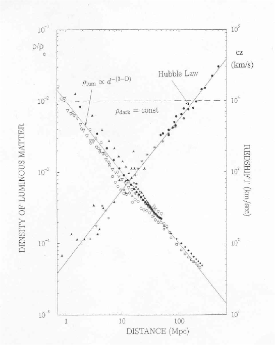
Figure 8: The Hubble law within the fractal galaxy distribution. From Baryshev et al. (1998).

A strong deflection from linearity expected within the fractal inhomogeneity cell was confirmed by Fang et al. (1991). The fractal aspect of this problem was discussed by Baryshev (1992, 1994) and Baryshev et al. (1998), who emphasized that the observed linear redshift-distance relation inside the power-law fractal density distribution creates the problem which they called the Hubble-deVaucouleur’s paradox, i.e. the observed coexistence of both laws on the same scales (see Fig.8). There are several possible solutions of the problem.

Asymptotically homogeneous LTB models. Using the LTB model Gromov et al. (2001) found the necessary conditions for the linear Hubble law existing within the fractal structure with fractal dimension $D=2$. The larger the scale of homogeneity $R_{hom}$ the smaller should be the density parameter $\Omega_{m}$, e.g. for $R_{hom}=100$ Mpc the linear Hubble law exists at distances $r>1$ Mpc if the density parameter $\Omega_{m}<0.01$.

Open Friedmann model. Joyce et al. (2000) suggested an open Friedmann model where the decreasing density of the fractal matter component at distance $R_{hom}$ becomes less than the density of the cosmic background radiation, which plays the role of the leading homogeneous component of the FRW universe. Hence the density parameter at the present epoch is $\Omega_{0}=\Omega_{rad}$ and space expands within the fractal structure. They also considered qualitatively the modifications to the physics of anisotropy of the CBR, nucleosynthesis and structure formation.

Influence of dark energy. Chernin et al. (2000), Chernin (2001), Baryshev et al. (2001) suggested that the cold local Hubble flow is a signature of the dominance of the cosmological vacuum or dark energy. Recent cosmological N-body simulations by Maccio et al.(2004) confirmed that inclusion of cosmic vacuum in the calculations leads to significantly lower velocity dispersion in Local Volume–like regions than what happens without vacuum.

6.2.2 Problem of the origin of the fractal structure

Since the 1970s Haggerty (1971), who worked in the University of Texas’ Center for Statistical Physics, has developed a Newtonian model for the creation of hierarchical self-gravitating structures. This was based on Prigogine’s and Severne’s study of a non-Markoffian kinetic theory of binary gravitational interactions with irreversible growth of correlational energy.

A scenario of explosive origing of large-scale structures was suggested by Ostriker & Cowie (1981) where large cavities and the superclusters of galaxies at scales up to 100 Mpc. This picture of galaxy formation is close to the way star formation is viewed. Within this approach Schulman & Seiden (1986) applied the percolation theory and numerical simulations for the derivation of the correlation exponent of the resulting structures. They got $\gamma\approx 1$ which corresponds to the fractal dimension $D\approx 2$. To obtain the commonly accepted value $\gamma=1.8$ they tried to find a mechanism for changing the initial slope.

Models for origins of the fractal large-scale structures were considered by Szalay & Schramm (1985), Pietronero & Kupers (1986), Maddox (1987), Luo & Schramm (1992).

Statistical mehanics and thermodynamics of self-gravitating gas was considered by Perdang (1990), de Vega et al. (1996, 1998), Combes (1998). The intriguing result is that Newtonian self-gravitating N-body systems have a quasi-equilibrium fractal state with a dimension of $\approx 2$, though several problems are still open and need more studies.

N-body simulations in order to study the gravitational growth and possible origin of fractal structures from initial small density fluctuations were made by Bottaccio et al. (2002), Baertschiger et al. (2002, 2004). They discovered that the discreteness has a strong influence on the results of standard cosmological simulations and noted that the Hubble time scale is too short for developing observed fractal structures within the whole range of scales.

Large density fluctuations even at high redshifts lead to a conflict with small temperature fluctuation of the CMBR and to the problem of formation time for largest structures. A possible solution is that the standard scenario of gravitational growth of large-scale structure from small initial density seeds should be revised. Also the observed anisotropy of CMBR can be essentially distorted by the interving matter, so the fractal initial conditions may not relate to the observed $\Delta T/T$ (Schwarz et al. 2004).

6.3 The Cosmological Principle

There is much confusion in the literature on how Mandelbrot’s Cosmological Principle of Fractality and its relation to the Einstein’s Cosmological Principle of Homogeneity should be understood. Below we compare these principles and show that the principle of fractality is a natural generalization of the principle of homogeneity.

6.3.1 Einstein’s Cosmological Principle

Einstein (1917) applied his general relativity to the cosmological problem, i.e. for constructing a model of the universe as a whole. Not yet knowing about galaxies, he imagined a world filled with stars and argued that the stars have a natural spatial distribution, which is uniform: matter concentrations around any preferred centre should with time evaporate and disperse uniformly all over the universe. Later, in correspondence with Selety, Einstein rejected the hierarchical distribution of stars (see sec.4.1).

Einstein postulated a uniform matter distribution, and put relativistic gravity into cosmology. The result was a world with uniform geometry. The Copernican cosmological principle has many faces, as has been interestingly discussed by Rudnicki (1995) in his book. Its one formulation “all places in the Universe are alike” is naturally fulfilled in a homogeneous world. Besides the absence of a centre, another plus-side of uniformity was a simplification of Einstein’s equations, which permitted him to derive the static spherical world model. Finally, Friedmann (1922) liberated the universe from this stiff state, allowing the uniformly distributed matter and space to expand.

The name Einstein’s Cosmological Principle for the hypothesis of the homogeneity of large scale matter distribution in the universe was coined by Edward Milne who analyzed the foundations of cosmology in the 1930s. Milne formulated also an observer-oriented version of the Cosmological Principle as: the whole world-picture as seen by one observer (attached to a fundamental particle or galaxy) is similar to the world-picture seen by any other observer.

In these early years of modern cosmology there was no direct observational evidence for the uniformity of the universe and it was theoretical reasoning which guided the cosmologist.

Modern view on the Cosmological Principle. Every cosmological model has its beginnings in cosmological principles, special kind of hypotheses which are regarded as valid for the whole, perhaps infinite universe, even though observations can be made only from a finite part of it. Some principles touch questions of epistemology and are tacitly supposed to be true, for example that the knowledge about the whole universe is accessible for us, and that the laws of physics are the same everywhere and produce similar things.

In the current cosmological thinking the contents of the Cosmological Principle are rather deep and complicated. We point out three distinct statements which are usually regarded as a starting point for constructing cosmological models.

• Physical laws the same in all space and time

• Fundamental physical constants are true constants

• Particular physical properties, including measuring standards, are the same in all space and time

When cosmology advances, these statements may require adjustments or even radical changes in the light of new observations and theoretical ideas. For example, multi-dimensional theories predict variations of physical constants. However, all modern observational tests strongly restrict any such variations (Uzan 2002). The requirement of the same physical laws (CP1) also includes the possibility of discovering new laws of cosmological physics which appear only on very large spatial, temporal and mass scales. An important principle ”More is Different” was introduced by Anderson (1972), who emphasized that each new level of complexity of material systems introduces new laws for their behaviour.

In modern cosmology the Cosmological Principle is understood in a narrow sense as a hypothesis on the large-scale distribution of matter in the universe. For example, the statement that matter has a homogeneous and isotropic distribution is at the basis of the standard cosmological model. Nowadays observations show that Mandelbrot’s cosmological principle of fractality has become an important alternative for the spatial distribution of luminous matter.

6.3.2 Derivation of uniformity from local isotropy

Walker (1944), a British mathematician who worked closely with Milne, proved that uniformity follows from his hypothesis of “Local Spherical Symmetry” which supposes that isotropy exists locally about each point of a Riemannian manifold.

A simple reasoning leading to homogeneity when there is isotropy around each point, may be found in the First Three Minutes by Weinberg (1977) . He shows how one can go from any one point to another arbitrary place along circle arcs on which the density remains the same. Hence the density is the same on every point. However, strictly speaking this conclusion is based on a hidden mathematical assumption of regularity, i.e. the existence of a smooth density around each point, only then from the left-hand side does the conclusion follow: Local Isotropy + No Centre + Regularity  $\Rightarrow$  Uniformity. Here “local isotropy plus no centre” means that all points are equivalent and around each point the density law does not depend on the direction (though it might depend on the distance from this point). The “regular” matter distribution is described by continuous, smooth mathematical functions.

In the chapter “Simplifying assumptions of cosmology” in his Introduction to Cosmology Narlikar (1993) explicitly introduces the assumption of the smooth fluid approximation, which essentially means going over from a discrete distribution of particles to a continuum density distribution. This is what we call “regularity”. It means that one may use the concept of the mass density at each point of space, like in a fluid. It is thus the union of local isotropy, no centre, and smoothness which gives homogeneity. In this case the Cosmological Principle reduces to the statement of the uniformity of the matter distribution.

6.3.3 Mandelbrot’s cosmological principle

In his book Fractals: form, chance, and dimension, Mandelbrot (1977) foresaw that galaxies are fractal-like distributed and gave the first mathematical description of the fractal properties of such a distribution. He recalls how around 1965, his ambition was to implement the law of decreasing density with a model where there is “no centre of the universe” or “the center is everywhere”.

Mandelbrot views the fractal galaxy distribution as a major conceptual step in the description of the cosmological matter distribution. It is a kind of synthesis of hierarchical structures (“thesis”) and homogeneity (“antithesis”), essentially based on randomness. Indeed, there is a fundamental difference between true random fractals and stiff hierarchical protofractals. Into protofractals the hierarchy is injected “ex-nihilo”, by defining explicitly its levels. But fractals internally contain a scale invariance (self-similarity) and the impression of a hierarchy follows as an unavoidable consequence. A useful example is the Lévy dust which is created by a random walk process in which the direction of each step is chosen isotropically and the length of a step follows a certain probability distribution.

Fractality carries within itself also a trace of uniformity. Within a fixed radius, i.e. for a fixed scale, every observer counts the same number of elements, on average. But upon changing the radius, a “new uniformity” is found with a new mean number density. Furthermore, there is no centre for random fractals – this is another “relic” from homogeneity.

Thus Mandelbrot made the first step for genuine fractals in cosmology, generalizing Einstein’s cosmological principle corresponding to $D=3$ by fractality, which allows a non-uniform galaxy distribution with $D<3$. His “Conditional Cosmographic Principle” states that all observers see similar cosmic landscapes around them, but only under the condition that they make observations from a structure element (galaxy). “Conditional” in the spatial context emphasizes that each observer occupies a material element of the structure (c.f. “conditional density”).

Mandelbrot’s cosmological principle of fractality – that the observers attached to the material structure elements are equivalent – is close to what Milne presented. Thus the fractality of the universe perfectly satisfies Milne’s Cosmological Principle. It also automatically makes what Karachentsev (1975) has called “the ecological correction to the Copernican principle” – the real observer can live only on or close to a material celestial body. This is usually called the Weak Anthropic Principle. In this sense the Copernican cosmological crinciple is contained by Mandelbrot’s principle of fractality and hence the assertions about an “unprincipled” fractal universe (see e.g. Coles 1998; Wu et al. 1999) are not true.

Does isotropy always imply uniformity? The proof of uniformity is based on the density being smooth around all points, which is valid for regular distributions, but not for fractals. It is smoothness which wipes out fractality and makes uniformity. Thus strictly speaking from local isotropy and the principle of no centre one can infer a fractality of the structure, of which homogeneity is only a special case with $D=3$ (see Sylos Labini, 1994).

Of course, there is never an exact local isotropy around every observer, not even in a uniform world, and still less inside a fractal distribution. Instead one may speak of a statistical isotropy, so that the sky observed from any galaxy “looks much the same”. In particular the counts of galaxies as a function of magnitude are similar around each galaxy, because radial distributions of galaxies are similar. It is natural to conjecture that for distributions made of discrete points, there is a generalization of the above chain of reasoning: Statistical Isotropy  +  No Centre  $\Rightarrow$  Fractality. Statistical isotropy and no centre, without the restrictive assumption of smooth mathematics, would thus lead to an isotropic fractal.

As considered in sec.2.4.5, the most important reason for an apparent isotropic celestial distribution of galaxies is the projection of a fractal structure with fractal dimension $D\geq 2$ . According to the theorem on fractal projections the resulting distribution will have the fractal dimension $D_{pr}=2$, which means homogeneity on a 2-d plane or isotropy on the celestial sphere.

Two other factors which lead to apparent isotropy on the sky are lacunarity and the luminosity function. It is now known that the patchiness on the sky depends not only on the fractal dimension, but also on the lacunarity, which is a measure of how frequent large voids are. Numerical simulations have shown that fractals with a small lacunarity can have rather smooth projections on the sky. The second factor which smooths out the patchiness, is the large differences in the luminosities of celestial bodies. As a result two objects with equal apparent brightness actually may have widely different distances. The mixing of nearby and distant objects hides clusters and fills in holes. For example, this decreases the celestial anisotropy for very distant radio sources.

6.3.4 Towards Einstein–Mandelbrot concordance

We do know of genuinely uniform components of the universe: the observed photon gas of the cosmic background radiation, the ocean of possible low-mass neutrinos, and maybe more importantly, the suggested physical vacuum or dark energy. As the average density of the fractal matter decreases with increasing scale, there will eventually be a scale beyond which the density of the uniform component is larger than the density of the fractal component. Hence one may regard, after all, the universe as homogeneous on such scales. However, this is not due to the galaxy distribution, but because of the uniformity of the relativistic matter component!

As to the fractal galaxy distribution, there are two alternatives – a finite or infinite range of fractality. True, there are no scale limits to a pure mathematical fractal. The name ‘fractal universe’ is often linked with an infinite fractal. Such a universe would have zero average density. But real physical objects usually have lower and upper cutoffs between which the fractal properties are observed. Thus it is also expected that the fractal galaxy distribution appears only within a finite interval of scales. One possibility is that it becomes homogeneous on some maximum scale $R_{\mathrm{hom}}$. Thus one may, as Mandelbrot did, allow for the possibility that the matter distribution may become uniform on large scales, while being fractal on smaller scales. With any uniform matter component, such as the photon-gas or the cosmological vacuum, the universe becomes homogeneous on a sufficiently large scale. Such a universe would have a non-zero average density. Thus the intuitions of both Einstein and Mandelbrot appear to have grasped fundamental features of the universe.

7 Concluding remarks

The historical milestones of the path of the study of the large-scale structure of the universe are outlined in Table 2. There one may see that during the period up to the 1970s many pioneering observational results and theoretical considerations appeared. The idea of a hierarchical matter distribution originated in a mathematical form thanks to Fournier, Charlier and Selety. It is intriguing to see that the problems discussed by Selety and Einstein in the 1920s, presently define whole directions in large-scale structure physics (see Table 3).

Observers discovered on the sky a very lumpy distribution of galaxies and prepared angular catalogues of galaxies and clusters, from which the first superclusters were detected up to sizes of 100 Mpc. These gathered clouds over homogeneous cosmological models and there was a sharp debate about the significance of such inhomogeneities. At the time when there was no extensive distance information, it seemed that convincing arguments for a homogeneous galaxy distribution were found. First, the number counts of bright galaxies appeared to agree with the $0.6m$ law of homogeneity. Second, fluctuations in Milky Way’s dust extinction was a factor producing apparent clustering. Third, the linearity of the Hubble law at small scales was seen as evidence for the galaxy homogeneity at similar small scales.

In the meanwhile, a conceptual breakthrough was the suggestion by Mandelbrot that the galaxy clustering may be described as a stochastic fractal. After the nature of spiral nebulae was settled, the discussion around the fractal dimension and the maximum scale of galaxy clustering forms the core of the new Great Debate.

During those early years the correlation function method, used in statistical physics for the description of homogeneous systems with small density fluctuations, was extensively applied to the angular distribution of galaxies. In an important step, Totsuji & Kihara (1969) discovered the power law dependence of the angular correlation function, with the exponent $\gamma=1.8$ and a small homogeneity scale $r_{0}=5h_{100}^{-1}$ Mpc. For a comprehensive description of the statistical results from the angular galaxy catalogue epoch see the review by Fall (1979) and the text-book by Peebles (1980).

Since then the correlation function has been applied for many angular and spatial galaxy catalogues, and in the words by Kerscher, Szapudi & Szalay (2000), “ the two-point correlation function became one of the most popular statistical tools in astronomy and cosmology”. These analyses created the feeling of confidence that the galaxy distribution is uniform on scales larger than $10h_{100}^{-1}$.

However, when the study of the galaxy clustering entered the new epoch of 3-d maps, a series of remarkable discoveries followed, which were unexpected in view of the 5 Mpc “correlation length”. The first findings of real spatial large scale structures up to 50 Mpc were reported at the Tallinn 1977 conference. After that larger and larger structures have been discovered up to our days, proving that the earlier detections of superclusters were not rare chance events, but actually probed essential properties of the galaxy clustering.

A decisive step was the introduction by Pietronero (1987) of the statistical method which is proper for the analysis of a fractal distribution of galaxies. This fractal-inspired method of conditional density has revealed the scale invariant galaxy clustering with the fractal dimension $D\approx 2$ up to scales where the method is applicable (Sylos Labini et al. 1998).

Also, it has become clear that the classical 2-point correlation function suffers from two major drawbacks. First, due to the projection effect the angular correlation function cannot detect spatial structures with the fractal dimension $D\geq 2$. Second, due to the normalization condition, both angular and spatial correlation functions yield systematically distorted values for the homogeneity scale ($\theta_{0}$, $r_{0}$) and the correlation exponent ($\gamma_{ang}$, $\gamma$), as compared with the true values of the complete correlation function. The importance of these effects is seen from the derivation of the correlation dimension $D_{2}=1.2$ from the $\xi$-method, when the $\Gamma$-method gives $D_{2}\approx 2$, for the main 3-d catalogues. The effects explain why the results from the $\xi$ and $\Gamma$ analyses have led to different conclusions about the homogeneity scale and the correlation exponent. These conflicting results on the value of the fractal dimension were also a cause for the controversy around the multifractal analysis of the galaxy data.

New extensive data, $200\,000$ galaxies for the 2dF survey (instead of 2000 for the CfA), together with the $\Gamma$ function analysis show that undistorted values of the correlation exponent is $\gamma\approx 0.8$ which corresponds to the fractal dimension $D=2.2\pm 0.2$. The scale of homogeneity $R_{\mathrm{max}}$ has a lower limit corresponding to the maximal sphere completely embedded into the volume of the galaxy survey, which is about $40h^{-1}_{100}$ Mpc for 2dF and $70h^{-1}_{100}$ Mpc for the first release SDSS. In order to obtain an estimate of $R_{\mathrm{hom}}$ on larger scales, one must enlarge the solid angle of the survey. Also, indirect evidence exist, such as the $450h^{-1}_{100}$ Mpc Sloan Great Wall and $300h^{-1}_{100}$ Mpc inhomogeneities in the 2dF QSO distribution, that $R_{\mathrm{hom}}$ could reach such large values. An application of the new method of the two-point conditional column density to the 2dF and SDSS data confirmed that $R_{hom}>100h^{-1}_{100}$ Mpc.

In order to obtain a reliable mass–radius relation $M(r)$ from observational data it is essential to use appropriate statistical methods of analysis (like conditional density $\Gamma(r)$) and control the distance scales $R_{sep}$ and $R_{max}^{sph}$ which determine the region of applicability of the used methods.

Three large numbers of galaxy redshift surveys needed for further progress in the large-scale sctructure analysis: large solid angle on the sky, large number of galaxies and large depth/separation ratio.

A special study of dark matter distribution is requiered, which now is possible by using gravitational lensing technics ( Mellier 1999; Wittman et al. 2000; Gray et al. 2002; Refregier 2003). The first results of the weak lensing analysis have shown that the dark and luminous matter are spatially similarly distributed.

We summarize the following main challenges that the modern galaxy clustering research faces:

• due to projection on the sky the angular distribution of galaxies loses the information on structures with fractal dimension $D\geq 2$;

• due to the normalization condition the $\xi$ function estimators yield incorrect values of the homogeneity scale $R_{\mathrm{hom}}$ and the fractal dimension $D$;

• the crucial role in statistical analysis of a galaxy sample plays the three quantities: the average distance between galaxies $R_{sep}$, the radius $R_{\mathrm{max}}^{\mathrm{sph}}$ of completely embedded spheres in the sample geometry, and the total number of galaxies $N_{gal}$ in VL subsamples;

• essential fluctuations in the derived value of $D$ are caused by the “cosmic variance” (only one realization of the stochastic process) and the “sampling variance” (finite available volume);

• the method of projected redshift-space correlation function cannot be applied to fractal structures with $D\geq 2$, hence new methods for extracting real-space correlation properties of the galaxy distribution are required;

• the pairwise velocity dispersion $500-600$ km/s on scales $1-10$ Mpc, obtained by the $\xi$-function method, is surprisingly high in comparison with the velocity dispersion $\sigma_{v}<100$ km/s in the Local Volume with $r<10$ Mpc;

• the differences in clustering of galaxies with different types and luminosities may require multifractal analysis;

• understanding the origin and evolution of the observed fractal distribution of galaxies may require a revision of the standard picture of gravitational growth of structure, by considering the consequences of primordial fractal density fluctuations.

We may conclude that the fractality of galaxy clustering has become a fundamental empirical phenomenon of observational cosmology, which should be explained by theoretical models of the Universe.

8 Acknowledgements

This work has been supported by Academy of Finland (project “Fundamental problems of observational cosmology”) and by the foundation Turun Yliopistosäätiö. We are grateful to Luciano Pietronero and Francesco Sylos Labini for valuable information, encouragement, and criticism. We also thank Fred Rost for very helpful comments.

References

- [1] Abell, G. O. 1958, The distribution of rich clusters of galaxies., ApJS. 3, 211
- [2] Abell, G. O. 1961, Evidence regarding second-order clustering of galaxies and interactions between clusters of galaxies, AJ 66, 607
- [3] Abell, G. O., Corwin, H.G., Olowin, R.P., 1989, A catalog of rich clusters of galaxies. ApJS 70,1
- [4] Alfvén, H., 1983, On hierarchical cosmology. Ap.Sp.Sci 89, 313
- [5] Ambartzumian, V.A., 1940, Fluctuations in numbers of extragalactic nebulae and Galactic extinction, Bulletin of Abastuman Observatory 4, 17 (in Russian)
- [6] Ambartzumian, V.A., 1951, On the theory of fluctuations in the apparent distribution of stars on the sky (in Russian), Communication of Burakan Observatory 6
- [7] Anderson, P.W., 1972, More is different. Science 177, 393
- [8] Axenides, M. & Perivolaropoulos, L., 2002, Dark energy and the quietness of the local Hubble flow. Phys. Rev. D 65, 127301 [astro-ph/0201524]
- [9] Baertschiger, T., Joyce, M., Sylos Labini, F., 2002, Power-law correlation and discreteness in cosmological N-body simulations. ApJ. 581, L63
- [10] Baertschiger, T., Sylos Labini, F., 2004, Growth of correlations in gravitational N-body simulations, Phys. Rev. D, 69, 123001-1
- [11] Bahcall, N.A., 1988, Large-scale structure in the universe indicated by galaxy clusters., ARA&A 26, 631
- [12] Bahcall, J.N. & Joss, P.C., 1976, Is the local supercluster a physical association?, ApJ 203, 23
- [13] Bahcall, N.A., Burgett, W.S., 1986, Are superclusters correlated on very large scale?, ApJ 300, L35
- [14] Bahcall, N.A., Dong, F., Hao, L. et al., 2003, The richness-dependent cluster correlation function: early sloan digital sky survey data. ApJ 599, 814
- [15] Bahcall,N.A., Soneira, R.M., 1983,The spatial correlation function of rich clusters of galaxies., ApJ 270, 20
- [16] Balian,R., Schaeffer, R., 1989, Scale-invariant matter distribution in the universe. A&A, 226, 373
- [17] Bardin, J.M., Bond, J.R., Kaiser, N., Szalay, A.S., 1986, The statistics of peaks of gaussian random fields. ApJ 3004, 15
- [18] Baryshev, Yu., 1981, The hierarchical structure of metagalaxy – a review of problems, Reports of Special Astrophysical Observatory of the Russian Academy of Sciences 14, 24 (English translation: 1984 Allerton Press)
- [19] Baryshev, Yu., 1992, “Modern state of observational cosmology”, VINTI, Itogi Nauki i Techniki, Series Classical Field Theory and Gravity Theory, vol.4: Gravitation and Cosmology p.89 (in Russian)
- [20] Baryshev, Yu., 1994, On the fractal nature of the large scale structure of the universe. Astron.Astrophys.Transactions 5, 15
- [21] Baryshev, Yu., 2000, Conceptual problems of fractal cosmology, Astron.Astrophys.Transactions 19, 417
- [22] Baryshev, Yu., 2003, The spatial distribution of galaxies and tests of relativistic cosmology, Doctor of Physical and Mathematical Sciences thesis, St.Petersburg University, St.Petersburg.
- [23] Baryshev, Yu., Bukhmastova, Yu., 2004, The method of a two-point conditional column density for estimating the fractal dimension of the distribution of galaxies, Astronomy Letters 30, 444
- [24] Baryshev, Yu., Ezova, Yu., 1997, Gravitational mesolensing by King objects and quasar–galaxy associations, Astronomy Reports 41, 436
- [25] Baryshev, Yu., Sylos-Labini, F., Montuori, M., Pietronero, L., 1994, Facts and ideas in modern cosmology, Vistas in Astronomy 38, 419
- [26] Baryshev, Yu. & Teerikorpi, P., 2002, Discovery of Cosmic Fractals (World Scientific Publishing, Singapore), 408pp
- [27] Baryshev, Yu., Chernin, A. & Teerikorpi, P., 2001, The cold local Hubble flow as a signature of dark energy A&A 378,729
- [28] Benoist, C., Maurogordato, S.,. da Costa, L.N., Cappi, A., Schaeffer, R., Biasing in the galaxy distribution., ApJ. 472, 452
- [29] Benzi, R., Paladin, G., Parisi, G., Vulpiani, A., 1984, J.Phys. A., 17, 3251
- [30] Best, J.S., 2000, An examination of the large-scale clustering of the Las Campanas redshift survey. ApJ 541, 519
- [31] Bharadwaj, S., Gupta, A.K., Seshadri, T.R., 1999, Nature of clustering in the Las Campanas redshift survey. A&A 351, 405
- [32] Biviano, A., 2000, From Messier to Abell: 200 years of science with galaxy clusters, in Constructing the Universe with Clusters of Galaxies, IAP 2000 meeting, Paris, eds. F. Durret & D. Gerbal; [astro-ph/0010409]
- [33] Blumenfeld, R., Mandelbrot, B.B., 1997, Lèvy dusts, Mittag-Leffler statistics, mass fractal lacunarity, and perceived dimension. Physical Review E 56, 112
- [34] Bondi, H., 1947, Spherically symmetrical models in general relativity, MNRAS 107, 410
- [35] Bonnor, W., 1972, A non-uniform relativistic cosmological model, MNRAS 159, 261
- [36] Bottaccio, M., Capuzzo-Dolcetta, R., Miocchi, P., Montuori, M., Pietronero, L., 2002, Europhys. Lett. 7, 315
- [37] Caldwell R.R., Dave R., Steinhardt P.J., 1998, Cosmological imprint of an energy component with general equation of state. Phys. Rev. Lett., 80, 1582
- [38] Caldwell R.R., Kamionkowski M., & Weinberg N.,N. 2003, Phantom energy and Cosmic Doomsday Phys.Rev.Lett. 91, 071301 [astro-ph/0302506]
- [39] Calzetti, D., Einasto, J., Giavalisco, M., Ruffini, R., Saar, E., 1987, The correlation function of galaxies in the direction of the Coma cluster. Ap.Sp.Sci 137, 101
- [40] Calzetti, D., Giavalisco, M., Ruffini, R., 1988, The normalization of the correlation functions for extragalactic structures. A&A 198, 1
- [41] Calzetti, D., Giavalisco, M., Ruffini, R., 1989, The angular two-point correlation functions and the cellular fractal structure of the Universe. A&A 226, 1
- [42] Carpenter, E.F., 1938, Some characteristics of associated galaxies I. A density restriction in the metagalaxy, ApJ. 88, 344
- [43] Charlier, C. 1908, Wie ein Unendliche Welt aufgebaut sein kann, Arkiv f. matematik, astronomi och fysik Band 4, N:o 24, p.1
- [44] Charlier, C. 1922, How an infinite world may be built up, Arkiv f. matematik, astronomi och fysik Band 16, N:o 22, p.1
- [45] Chernin, A., 2001, Cosmic vacuum, Physics-Uspekhi, 44, 1153
- [46] Chernin, A., Karachentsev, I., Valtonen, M., Dolgachev, V., Domozhilova, L., Makarov, D. 2004, The very local Hubble flow: computer simulations of dynamical history. A&A 415, 19
- [47] Chernin, A., Teerikorpi, P., Baryshev Yu., 2000, Why is the Hubble flow so quiet?, astrp-ph/0012021
- [48] Chiang L.Y., Coles P., 2000b Phase information and the evolution of cosmological density perturbations, Mon.Not.Roy.Astron.Soc., v.311, 809
- [49] Coleman, P.H., Pietronero, L., Sanders, R.H., 1988, Absence of any characteristic correlation length in the CfA galaxy catalogue. A&A 200, L32
- [50] Coleman, P.H., Pietronero, L., 1992, The fractal structure of the Universe, Phys.Rep. 213, 311
- [51] Coles, P., 1998, An unprincipled universe? Nature 391, 120
- [52] Coles, P., Chiang,L.Y., 2000, Characterizing the nonlinear growth of large-scale structure in the Unverse, Nature 406, 376
- [53] Colless M., Dalton G., Maddox S. et al. (the 2dFGRS team), 2001, The 2dF Galaxy Redshift Survey: spectra and redshifts, MNRAS, 328, 1039
- [54] Colless M. and the 2dFGRS team, 2003, astro-ph/0306581
- [55] Combes, F., 1998, Fractal structure driven by self-gravity: molecular clouds and the Universe. astro-ph/9804048
- [56] Conklin, E.K. & Bracewell, R.N., 1967, Isotropy of Cosmic Background Radiation at 10 690 MHz. Phys.Rev.Letts. 18, 614
- [57] Courtois, H., Paturel, G., Sousbie, T., Sylos Labini, F., 2004a, The LEDA galaxy distribution: I. Maps of the Local Universe. A&A 423, 27
- [58] Courtois, H., Sousbie, T., Sylos Labini, F., Paturel, G., Le Delliou, M., 2004b, The LEDA galaxy distribution: II. Correlations in the Local Universe. A&A (in preparation)
- [59] Da Costa, L.N. et al., 1991, Southern sky redshift survey: the catalog. ApJS 75, 935
- [60] Da Costa, L.N. et al., 1994, A complete southern sky redshift survey. ApJ 424, L1
- [61] Davis, M., 1997, in the Proc. of the Conference “Critical Dialogues in Cosmology”, ed. Turok, N., p.13 (World Scientific, Singapore, 1997)
- [62] Davis, M., Peebles, P.J.E., 1983, A survey of galaxy redshifts. V.The two-point position and velocity correlations. ApJ. 267, 465
- [63] Davis, M., Meiksin, A., Strauss, M.A., da Costa, L.N., Yahil, A., 1988, On the universality of the two-point galaxy correlation function. ApJ. 333, L9
- [64] Di Nella, H., Paturel, G., 1994, Large-scale structure of the Universe up to a distance of 200 Mpc. C.R. Acad. Sc. Paris, t. 319, Sér.II, 57
- [65] Dogterom, M., Pietronero, L., 1991, Physica A 171, 239
- [66] Durrer, R., Eckmann, J.-P., Sylos Labini, F., Montuori, M., Pietronero, L., 1997, Angular projections of fractal sets. Europhys.Lett. 40, 491
- [67] Eckmann, J.-P., Järvenpä”a, E., Järvenpä”a, M., Procaccia, I., On the fractal dimension of the visible universe. In Simplicity Behind Complexity (Euroattractor 2002), ed. W. Klonowski (Pabst Science Publishers, Lengerich 2004)
- [68] Einasto, J., Klypin, A., Saar, E.,1986, Structure of superclusters and supercluster formation – V. Spatial correlation and voids., MNRAS 219, 457
- [69] Einstein, A., 1917, Kosmologische Betrachtungen zur allgemeinen Relativitatstheorie, Sitzungsber. d. Berl. Alead. 1, 142
- [70] Einstein, A, 1922, Bemergung zur Seletyschen Arbeit: Beitr ge zum kosmologischen Problem, Annalen der Physik, Ser.4, Vol. 69, p.436
- [71] Ekholm, T., Baryshev, Yu., Teerikorpi, P., Hanski, M. & Paturel, G., 2001, On the quiescence of the Hubble flow in the vicinity of the Local group: a study using galaxies with distances from the Cepheid PL-relation. A & A 368, L17
- [72] Ekholm, T., Lanoix P., Paturel G., Teerikorpi, P., Fouque P., 1999, Investigations of the Local Superclaster velocity field: II. A study using Tolman-Bondi solution and galaxies with accurate distances from the Cepheid PL-relation, A & A 351, 827
- [73] Fairall, A., 1998, Large-scale structures in the universe, John Wiley & Sons
- [74] Fall, S.M., 1979, Galaxy correlations and cosmology, Reviews of Modern Physics 51, 21
- [75] Fall, S.M. & Tremaine, S., 1977, On estimating correlations in the spatial distribution of galaxies. ApJ 216, 682
- [76] Fang, L.L., Mo, H.J., Ruffini, R., 1991, The cellular structure of the universe and cosmological tests. A&A 243, 283
- [77] Fesenko, B.I., 1975, The galactic extinction from the apparent distribution of galaxies. Soviet Astronomy 19, 177
- [78] Feynman R., Morinigo F., Wagner W., 1995, Feynman Lectures on Gravitation, Addison-Wesley Publ. Comp.
- [79] Fischer, K., et al., 1996, The IRAS 1.2 Jy survey: redshift data. ApJS. 100, 69
- [80] Fournier d’Albe, E., 1907 Two New Worlds (Longmans Green, London, 1907)
- [81] Friedmann, A., 1922, On the curvature of space, Zeits. f. Physik, 10, 377
- [82] Friedmann, A., 1924, On a possibility of world with constant negative curvature of space, Zeits. f. Physik, 21, 326, 1924.
- [83] Gabrielli, A., Sylos Labini, F., Durrer, R., 2004, Biasing in Gaussian random fields and galaxy correlations. ApJ 531, L1
- [84] Gabrielli, A., Sylos Labini, F., Joyce, M., Pietronero L., 2004, Statistical Physics for Cosmic Structures, Springer Verlag
- [85] Geller, M. & Huchra, J., 1989, Science 246, 897
- [86] Giovanelli, R., Haynes, M., 1991, Redshift surveys of galaxies. Ann.Rev.Astron. Astrophys. 29, 499
- [87] Gott, J.R., Juric, M., Schlegel, D. et al., 2003, A map of the universe. [astro-ph/0310571]
- [88] Governato, F., Moore, B., Cen, R., Stadel, J., Lake, G., Quinn, T., 1997, The Local Group as a test of cosmological models. New Astronomy 2, 91
- [89] Gray M., Taylor A., Meisenheimer K., Dye S., Wolf G., Thommes E., 2002, Probing the distribution of dark matter in the A901/902 supercluster with weak lensing, ApJ 568, 141
- [90] Gromov, A., Baryshev, Yu., Suson, D. & Teerikorpi, P., 2001, Lemaitre-Tolman- Bondi model: fractality, non-simultaneus bang time and the Hubble law. Gravitation & Cosmology 7, 140
- [91] Gromov, A., Baryshev, Yu., Teerikorpi, P., 2004, Two- fluid matter-quintessence FLRW models: energy transfer and the equation of state of the universe, A&A, 415, 813
- [92] Grujić, 2001, The concept of fractal cosmos: I. Anaxagoras’s cosmology, Serbian Astr.J., N.163, 21
- [93] Grujić, 2002, The concept of fractal cosmos: II. modern cosmology, Serbian Astr.J., N.165, 45
- [94] Haggerty, M.J., 1971, A Newtonian model for the creation of a hierarchical cosmology. ApJ 166, 257
- [95] Haggerty, M.J., Wertz, J.R., 1972, On the redshift– magnitude relation in hierarchical cosmologies. MNRAS 155, 495
- [96] Harrison, E. R., 1987, Darkness at Night (Harvard University Press )
- [97] Harrison, E. R., 2000, Cosmology – the Science of the Universe, 2nd edition (Cambridge University Press 2000)
- [98] Haynes, M., Giovanelli, R., 1988, “Large-scale motion in the Universe”, eds. Rubin, V.C., Coyne, G., Princeton University Press, Princeton.
- [99] Hawkins, E., Maddox, S., Cole, S. et al., 2003, The 2dF Galaxy Redshift Survey: correlation functions, peculiar velocities and the matter density of the Universe., MNRAS 346, 78
- [100] Hogg D., Eisenstein D., Blanton M. et al., 2004, Cosmic homogeneity demonstrated with luminous red galaxies. astro-ph/0411197
- [101] Holden, D.J., 1966, An investigation of the clustering of radio sources. MNRAS 133, 225
- [102] Holmberg, E., 1974, Distribution of clusters of galaxies as related to galactic absorption, A&A 35, 121
- [103] Hubble, E., 1926, Extra-galactic nebulae. ApJ 64, 321
- [104] Hubble, E., 1929, A relation between distance and radial velocity among extra-galactic nebulae. Proceed. Nat. Acad. Sci., 15, 168
- [105] Hubble, E., 1934, The distribution of extra-galactic nebulae. ApJ 79, 8
- [106] Hubble, E., 1936, Effects of red shifts on the distribution of nebulae. ApJ 84, 517
- [107] Hubble, E., 1937, The Observational Approach to Cosmology, The Clarendon Press, Oxford (68pp)
- [108] Huber D., Pfenniger D. 2001, Long-range correlations in self-gravitating N-body systems. astro-ph/0105501
- [109] Huchra, J., Geller, M., de Lapparent, V. & Burg, R., 1988, The Center for Astrophysics redshift survey. in Large Scale Structures of the Universe, IAU Symposium 130, (eds. J. Audouze, M.-C. Pelletan & A. Szalay), p.105
- [110] Humason, M.L., 1931, Apparent velocity-shifts in the spectra of faint nebulae. ApJ 74, 35
- [111] Joeveer, M. & Einasto, J., 1978, Has the Universe the Cell Structure? in The Large-Scale Structure of the Universe, IAU Symposium 79 (eds. M. Longair, J. Einasto), p.241
- [112] Jones, B., Coles, P., Martinez, 1992, Heterotopic clustering. MNRAS 259, 146
- [113] Jones, B., Martinez, V., Saar, E., Einasto, J., 1988, Multifractal description of the large-scale structure of the universe. ApJ 332, L1
- [114] Jones, B., Martinez, V., Saar, E., Trimble, V., 2004, Scaling laws in the distribution of galaxies, Rev. Mod. Phys., 76, 1211 [astro-ph/0406086]
- [115] Joyce, M., Anderson, P.W., Montuori, M., Pietronero, L., Sylos Labini, F., 2000, Fractal cosmology in an open universe, Europhys. Lett., 50, 416
- [116] Joyce, M., Montuori, M., Sylos Labini, F., 1999, Fractal correlations in the CfA2-south redshift survey. ApJ 514, L5
- [117] Joyce, M., Sylos Labini, F., 2001, Luminosity density estimation from redshift surveys and the mass density of the universe. ApJ 554, L1
- [118] Joyce, M., Sylos Labini, F., Gabrielli A., Montuori M., Pietronero L., 2005, Basic properties of galaxy clustering in the light of recent results from the SDSS, astro-ph/0501583
- [119] Kaiser, N., 1984, On the spatial correlations of Abell clusters., ApJ 284, L9
- [120] Kant, I., Allgemeine Naturgeschichte und Theorie des Himmels. English translation Universal Natural History and Theory of the Heavens (transl. S.L.Jaki) (SCottish Academic Press, Edingburgh, 1981) See also http://www.mala.bc.ca/ johnstoi/kant1.htm.
- [121] Karachentsev, I.D., 1966, Some statistical characteristics of superclusters of galaxies. Astrofizika 2, 307 (English translation in Astrophysics 2, 159)
- [122] Karachentsev, I.D., 1968, Average statistical characteristics of systems of galaxies and the problem of the existence of hidden virial mass. Communications of Burakan Observatory 39, 76 (in Russian)
- [123] Karachentsev, I.D., 1975, Acta Cosmologica 2, 43
- [124] Karachentsev I. & Kopylov A., 1988, A cut of large-scale structure across the Coma supercluster, in Large Scale Structures of the Universe, IAU Symposium 130, (eds. J. Audouze, M.-C. Pelletan & A. Szalay), p.139
- [125] Karachentsev, I.D., Lipovetskii, V.A., 1969, Absorbing material in clusters of galaxies. Sov.Astronomy 12, 909
- [126] Karachentsev, I.D. & Makarov, D.A., 1996, The Galaxy motion relative to nearby galaxies and the local velocity field. AJ 111, 794
- [127] Karachentsev, I., Chernin, A., Teerikorpi, P., 2003a, The Hubble flow: why does the cosmological expansion preserve its kinematical identity from a few Mpc distance to the observation horizon? Astrofizika 46, 491
- [128] Karachentsev, I., Drozdovsky, I., Kajsin, S. et al., 1997, Revised photometric distances to nearby dwarf galaxies in the IC342/Maffei complex. AASS 124, 559
- [129] Karachentsev, I., Makarov, D.I., Sharina, M.E. et al., 2003b, Local galaxy flows within 5 Mpc. A&A 398, 479
- [130] Karachentsev, I.D., Sharina, M.E., Makarov, D.I., 2002, The very local Hubble flow. A&A 389, 812
- [131] Karachentsev, I.D., Tikhonov, N.A., 1994, New photometric distances for dwarf galaxies in the Local Volume. A&A 286, 718
- [132] Karachentseva, V.E. & Karachentsev, I.D., 1998, A list of new nearby dwarf galaxy candidates, AASS 127, 409
- [133] Karachentseva, V.E.,& Karachentsev, I.D., 2000, A supplementary list of southern nearby dwarf galaxy candidates, AASS 146, 359
- [134] Kerscher, M., Szapudi, I. & Szalay, A.S., 2000, A comparison of estimators for the two-point correlation function. ApJ 535, L13
- [135] Kiang, T., 1967, On the clustering of rich clusters of galaxies. MNRAS 135, 1
- [136] Kiang, T., Saslaw, W.C., 1969, The distribution in space of clusters of galaxies. MNRAS 143, 129
- [137] Kilborn, V.A., Webster, R.L., Staveley-Smith, L. et al., 2002, A catalog of HI-selected galaxies from the South Celestial Cap Region of sky. 2002, AJ 124, 690
- [138] Klypin, A., Einasto, J., Einasto M., Saar, E., 1989, Structure and formation of superclusters – X: Fractal properties of superclusters. MNRAS 237, 929
- [139] Klypin, A.A., Kopylov, A.I., 1983, The spatial covariance function for rich clusters of galaxies. Sov.Astron.Lett. 9, 41
- [140] Klypin, A., Hoffman, Y., Kravtsov, A., Gottloeber, S., 2003, Constrained simulations of the real Universe: the Local Supercluster. ApJ 596, 19
- [141] Kopylov A., Kuznetsov D., Fetisova T. & Shvartsman V., 1988, Possible inhomogeneities in the Universe on scales of 100 – 300 Mpc from observations with the 6-meter telescope, in Large Scale Structures of the Universe, IAU Symposium 130, (eds. J. Audouze, M.-C. Pelletan & A. Szalay), p.129
- [142] Kraan-Korteweg, R.C. & Lahav, O., 2000, The Universe behind the Milky Way. A&ARev. 10, 211
- [143] Kraan-Korteweg, R.C & Tammann, G., 1979, A catalogue of galaxies within 10 Mpc. Astron.Nachrichten 300, 181
- [144] Lambert, J.H., Kosmologischen Briefen (Cosmological Letters), Ausburg 1761. Printed in G. Jackisch: J.H. Lamberts Cosmologische Briefe (Akademie-Verlag, Berlin 1979)
- [145] Landau, L.D., Lifshitz, E.M., 1958, Statistical Physics (Pergamon, London)
- [146] Landau, L.D., Lifshitz, E.M., 1971, The Classical Theory of Fields (Pergamon, Oxford)
- [147] de Lapparent, V. et al., 1988, The mean density and two-point correlation function for the CfA redshift survey. ApJ 332, 44
- [148] Lebedev, V., Lebedeva, I., 1988, The spatial correlation functions of superclusters of galaxies., Sov.Atron.Lett. 14, 18
- [149] Lemson, G. & Sanders, R.H., 1991, On the use of the conditional density as a description of galaxy clustering. MNRAS 252, 319
- [150] Lerner, E., 1986, Magnetic vortex filaments, universal invariants, and the fundamental constants. IEEE Transactions on Plasma Science; Special Issue on Cosmic Plasma, vol. PS-14, p. 690
- [151] Limber, D.N., 1953, The analysis of counts of the extragalactic nebulae in terms of a fluctuating density field. ApJ 117, 134
- [152] Longair, M.S., 1978, Personal view - the large scale structure of the Universe, in The Large-Scale Structure of the Universe, IAU Symposium 79 (eds. M. Longair, J. Einasto), p.451
- [153] Loveday, J., Peterson, B.A., Efstathiou, G., Maddox, J.S., 1992, The Stromlo-APM redshift survey. I. The luminosity function and space density of galaxies. ApJ. 390, 338
- [154] Loveday J. and SDSS collaboration, 2002, The Sloan Digital Sky Survey, astro-ph/0207189
- [155] Lundmark, K., 1924, The determination of the curvature of space-time in de Sitter’s world, MNRAS 84, 747
- [156] Lundmark, K., 1927, Studies of anagalactic nebulae. Medd. f. Astron. Obs. Upsala N:o 30
- [157] Luo, X. & Schramm, D.N., 1992, Fractals and cosmological large-scale structure. Science 256, 513
- [158] Maccio, A, Governato, F., Horellow, C., 2004, The signature of dark energy on the local Hubble flow. astro-ph/0412583
- [159] Maddox, J., 1987, The universe as a fractal structure. Nature 329, 195
- [160] Madgwick D. et al., 2003, MNRAS, 344, 847
- [161] Mandelbrot, B.B., 1975, Les Objects Fractals: Forme, Hasard et Dimension,Paris & Montreal, Flammarion
- [162] Mandelbrot, B. B., 1977, Fractals: Form, Chance and Dimension, W. H. Freeman, New York
- [163] Mandelbrot, B. B., 1982, The fractal geometry of nature, W. H. Freeman, New York
- [164] Mandelbrot, B. B., 1988, Fractals and Multifractals: Noise, Turbulence and Galaxies, Springer, New York
- [165] Mandelbrot, B.B., 1989, The fractal range of the distribution of galaxies; crossover to homogeneity, and multifractals. In M. Mezzetti et al. (eds.), Large Scale Structure and Motions in the Universe (Kluwer Academic Publishers), p. 259
- [166] Martinez, V.J., Jones, B.J.T., 1990, Why the universe is not a fractal. MNRAS 242, 517
- [167] Martinez, V.J., Lopez-Marti, B., Pons-Borderia, M.-J., 2001, Does the correlation length increase with the sample depth?, ApJ 554, L5
- [168] Martinez, V.J., Saar, E., 2002, Statistics of the Galaxy Distribution, Chapman & Hall/CRC
- [169] Mattila, K., 1977, Photometry of the intergalactic optical surface brightness in the Coma cluster. A&A 60, 425
- [170] Mellier, Y., 1999, Probing the Universe with weak lensing, ARAA 37, 127
- [171] Montuori, M., Sylos Labini, F., 1997, Angular correlations of galaxy distribution. ApJ 487, L21
- [172] Moore, B., Calcaneo-Roldan, C., Stadel, J., Quinn, T., Lake, G., Ghigna, S., Governato, F., 2001, Dark matter in Draco and the Local Group: Implications for direct detection experiments. Phys.Rev. D64 063508
- [173] Narlikar, J., 1993, Introduction to Cosmology, 2nd edition (Cambridge University Press, Cambridge)
- [174] Neyman, J., Scott, E.L., 1952, A theory of the spatial distribution of galaxies, ApJ 116, 144
- [175] Norberg, P., Baugh, C.M., Hawkins, E., et al., 2001, The 2dF Galaxy Redshift Survey: Luminosity dependence of galaxy clustering., MNRAS 328, 64
- [176] Norberg, P., Baugh, C.M., Hawkins, E., et al., 2002, The 2dF Galaxy Redshift Survey: The dependence of galaxy clustering on luminosity and spectral type. MNRAS 332, 828
- [177] Paladin, G., Vulpiani, A., 1987, Anomalous scaling laws in multifractal objects. Phys.Rep. 156, 147
- [178] Park, C., Vogeley, M.S., Geller, M.J., Huchra, J.P., 1994, Power spectrum, correlation function, and tests for luminosity bias in the CfA redshift survey., ApJ 431, 569
- [179] Paturel, G., Bottinelli, L., Gouguenheim, L., Fouqué, P.,1988, New determination of the pole of a “Hypergalactic” large scale system. A&A 189, 1
- [180] Paturel G., Bottinelli L., Di Nella H., Gouguenheim L., Teerikorpi P., 1994, Kinematics of the Local Universe: Completeness of the sample; A&A 289, 711
- [181] Paturel G., Di Nella H., 1995, Galaxy distribution around the Local Super Cluster. Astrophys.Letters and Comm. 31, 337
- [182] Paturel G., Bottinelli L., Di Nella H. et al., 1997, The Extragalactic Data Base: VII - Reduction of astrophysical parameters. A&ASS 124, 109
- [183] Peacock J.A., 1999, Cosmological Physics, Cambridge Univ. Press
- [184] Peebles, P.J.E., 1974a, The gravitational instability picture and the nature of the distribution of galaxies. ApJ 189, L51
- [185] Peebles, P.J.E., 1974b, A model for continuous clustering in the large-scale distribution of matter. Ap.Sp.Sci 31, 403
- [186] Peebles, P.J.E., 1978, Large scale clustering in the Universe, in the Proc. of IAU Symp.N79 The Large Scale Structure of the Universe, eds. M.S.Longair and J.Einasto, D.Reidel, Dordrecht, 1980, p.217
- [187] Peebles, P.J.E., The Large-Scale Structure of the Universe, Princeton Univ. Press. Princeton, 1980.
- [188] Peebles, P.J.E., 1988, Summary, in Large Scale Structures of the Universe, IAU Symposium 130, (eds. J. Audouze, M.-C. Pelletan & A. Szalay), p.495
- [189] Peebles, P.J.E., Principles of Physical Cosmology, Princeton Univ. Press. Princeton, 1993.
- [190] Peebles, P.J.E., 2001, The galaxy and mass N-point correlation functions: a blast from the past. in Historical Developments of Modern Cosmology ASP Conference Series, eds. V.J. Martinez, V. Trimble, M.J. Pons-Borderia; astro-ph/0103040
- [191] Peebles, P.J.E., 2002, From precision cosmology to accurate cosmology. astro-ph/0208037
- [192] Peebles, P.J.E., 2003, Open problems in cosmology, astro-ph/0311435
- [193] Peebles, P.J.E., Ratra B., 2003, The cosmological constant and dark energy, Rev.Mod.Phys. 75, 599 astro-ph/0207347, 2002.
- [194] Penzias, A.A., Schraml, J., Wilson, R.W., 1969, Observational constraints on a discrete-source model to explain the microwave background. Ap.J.Lett. 157, L49
- [195] Perdang, J., 1990, Self-gravitational fractal configuration, Vistas in Astronomy 33, 371
- [196] Pietronero, L., 1987, The fractal structure of the Universe: correlations of galaxies and clusters and the average mass density. Physica A., 144, 257
- [197] Pietronero, L., Kupers, R., 1986, Stochastic approach to large scale clustering of matter in the universe. in Fractals in physics, eds. L. Pietronero, E. Tosatti (Elsevier Science Publ., Amsterdam), p. 319
- [198] Pietronero, L., Montuori, M., Sylos Labini, F., 1997, in the Proc. of the Conference “Critical Dialogues in Csomology”, ed. Turok, N., p.24 (World Scientific, Singapore, 1997)
- [199] Refregier A., 2003, Weak gravitational lensing by large-scale structure, ARAA 41, 645
- [200] Ribeiro, M.B., 1992, On modeling a relativistic hierarchical (fractal) cosmology by Tolman’s spacetime. I. Theory., ApJ 388, 1
- [201] Ribeiro, M.B., 1993, On modeling a relativistic hierarchical (fractal) cosmology by Tolman’s spacetime. III. Numerical results. ApJ 415, 469
- [202] Rost, F., 2004, Estimates of the fractal dimension and density of the Universe from the empirical mass-radius relation in cluster systems. (in preparation)
- [203] Rudnicki, K., 1995, The Cosmological Principles, Jagiellonian University, Cracow
- [204] Ruffini, R., Song, D.J., Taraglio, S., 1988, The “ino” mass and the cellular large-scale structure of the Universe. AA 190, 1
- [205] Sandage, A., 1961, The ability of of the 200-inch telescope to discriminate between selected world models. ApJ 133, 355
- [206] Sandage, A., 1962, The change of redshift and apparent luminosity of galaxies due to the deceleration of the expanding universes. ApJ 136, 319
- [207] Sandage, A., 1986, The redshift-distance relation.IX. ApJ 307, 1
- [208] Sandage, A., 1987, The redshift-distance relation.IXa. ApJ 317, 557
- [209] Sandage, A., 1988, Observational tests of world models, Ann. Rev. Astron. Astrophys. 26, 561
- [210] Sandage, A., 1992, The Search for the Curvature of Space, Physica Scripta, Vol. T43, 7
- [211] Sandage A. ,1995a, Astronomical problems for the next three decades. In Key Problems in Astronomy and Astrophysics, Mamaso A. and Munch G. eds., Cambridge University Press
- [212] Sandage, A., 1995b, in The Deep Universe, eds.B. Binggeli, R. Buser (Springer)
- [213] Sandage, A., 1999, Bias Properties of Extragalactic Distance Indicators. VIII, from Distance-limited Luminosity Class and Morphological Type-Specific Luminosity Functions for Sb, Sbc, and Sc Galaxies Calibrated Using Cepheids, ApJ. 527, 479
- [214] Sandage, A., 2004, Breaking the Code of Cosmic Evolution: An Informal History of the Mount Wilson Observatory (1904–1950), Cambridge University Press
- [215] Sandage, A. & Tammann, G.A., 1975, Steps toward the Hubble Constant. V. The Hubble constant from nearby galaxies and the regularity of the Local Velocity Field. Ap.J. 196, 313
- [216] Sandage, A., Tammann, G.A., Hardy, E., 1972, Limits on the local deviation of the Universe for a homogeneous model. ApJ 172, 253
- [217] Saslaw, W., 2000, The Distribution of the Galaxies – Gravitational Clustering in Cosmology (Cambridge University Press 2000)
- [218] Schulman, L.S., Seiden, P.E., 1986, Hierarchical structure in the distribution of galaxies. ApJ 311, 1
- [219] Schwarz D., Starkman G., Huterer D., Copi C., 2004, Is the low-l microwave background cosmic? Phys.Rev.Lett., 93, 221301 (astro-ph/0403353)
- [220] Seeliger, H. von, 1895, Ueber das Newton’sche Gravitationsgesetz. Astronomische Nachrichten 137, 9
- [221] Selety, F.J., 1922, Beiträgen zum kosmologischen Problem, Annalen der Physik Band 68, N:o 12, p. 281
- [222] Selety, F.J., 1923, Erwiderung auf die Bemergungen Einsteins über meine Arbeit “Beiträgen zum kosmologischen Problem”, Annalen der Physik Band 72, N:o 17, p. 58
- [223] Shane, C.D., Wirtanen, C.A., 1967, The distribution of galaxies, Publ. Lick Obs., 22, Part 1.
- [224] Shapley, H., 1943, Galaxies (The Blakiston Company)
- [225] Shapley, H., Ames, A., 1932, A survey of the external galaxies brighter than the thirteenth magnitude, Ann. Harvard Coll. Obs. 88, No.2
- [226] Shapley, H., 1957, The Inner Metagalaxy Yale University Press, New Haven, 204pp
- [227] Shapley, H. & Shapley, M.B., 1919, Studies based on the colors and magnitudes in stellar clusters. Fourteenth paper: Further remarks on the structure of the galactic system., ApJ 50, 107
- [228] Shectman, S.A. et al., 1996, The Las Campanas redshift survey. ApJ 470, 172
- [229] Sidharth, B, 2000, The fractal Universe. [physics/0004001]
- [230] Smith, R.W., 1983, The Great Debate revisited. Sky & Telescope January 1983, p. 28
- [231] Soneira, R.M., Peebles, P.J.E., 1977, Is there evidence for a spatially homogeneous population of field galaxies?, ApJ 211, 1
- [232] Soneira, R.M., Peebles, P.J.E., 1978, A computer model universe: simulation of the nature of the galaxy distribution in the Lick catalog, AJ 83, 845
- [233] Stickel, M., Lemke, D., Mattila, K., Haikala, L.K., Haas, M., 1998, Far-infrared emission of intracluster dust in the Coma galaxy cluster. A&A 329, 55
- [234] Strauss, M.A. et al., 1992, A redshift survey of IRAS galaxies. VII. The infrared and redshift data for the 1.936 Jansky sample. ApJS 83, 29
- [235] Sylos Labini, F., 1994, Isotropy, homogeneity, and dipole saturation. ApJ 433, 464
- [236] Sylos Labini, F., Amendola, L., 1996, The power spectrum in a strongly inhomogeneous Universe, ApJ 468, L1
- [237] Sylos Labini, F., Pietronero, L., 1996, Multifractality as a link between luminosity and space distribution of visible matter, ApJ 469, 26
- [238] Sylos Labini, F., Montuori M., Pietronero, L., Scale-invariance of galaxy clustering. Phys. Rep., v. 293, 61-226, 1998.
- [239] Szalay, A.S. & Schramm, D.N., 1985, Are galaxies more strongly correlated than clusters? Nature 314, 718
- [240] Teerikorpi, P., 1975a, A note on the velocity–distance relationship for nearby galaxies and galaxy groups. Observatory 95, 105
- [241] Teerikorpi, P., 1975b, On the effect of the luminosity selection on the redshift–distance relationship. A&A 45, 117
- [242] Teerikorpi, P., 1982, Studies of the Hubble Law with emphasis of selection effects and Galactic absorption Rep.Ser. No.D4, Dep.Phys.Sci., Univ. Turku
- [243] Teerikorpi, P., 1997, Observational selection bias affecting the determination of the extragalactic distance scale, ARAA 35, 101
- [244] Teerikorpi, P., 2001, Dark haloes in Karachentsev’s sample of binary galaxies. A&A 371, 470
- [245] Teerikorpi, P., 2002, Dusty haloes of galaxies at intermediate redshifts. A&A 386, 865
- [246] Teerikorpi, P., 2004, Influence of a generalized Eddington effect on galaxy counts. A&A 424, 73
- [247] Teerikorpi, P., Bottinelli, L., Gouguenheim, L., Paturel, G. 1992, Investigations of the local supercluster velocity field: I. Observations close to Virgo, using Tully-Fisher distances, and the Tolman-Bondi expanding sphere, A&A 260, 17
- [248] Teerikorpi, P., Hanski, M., Theureau, G., Baryshev, Yu., Paturel, G., Bottinelli, L., Gouguenheim, L., 1998, The radial space distribution of KLUN-galaxies up to 200 Mpc: incompleteness or evidence for the behaviour predicted by fractal dimension ? A&A 334, 395
- [249] Teerikorpi, P., 2003, Evidence for the class of the most luminous quasars IV. Cosmological Malmquist bias and the term, A&A 399, 829
- [250] Tegmark, M., Blanton, M., Strauss, M. 2004, The three-dimensional power spectrum of galaxies from the Sloan Digital Sky Survey. Ap.J., 606, 702
- [251] Tegmark M., Hamilton A., Xu Y., 2002, The power spectrum of galaxies in the 2dF 100k redshift survey, MNRAS, 335, 887
- [252] Theureau, G., Hanski, M., Ekholm, T. et al, 1997, Kinematics of the Local universe. V. The value of from the Tully–Fisher and relations for field galaxies. A&A 322, 730
- [253] Theureau, G., Coudreau, G., Hallet, N. et al., 2004, Kinematics of the Local Universe XII. 21-cm line measurements of 586 galaxies with the new Nancay receiver. A&A (in press)
- [254] Tikhonov, A., Makarov, D., Kopylov, A., 2000, Investigation of the clustering of galaxies, clusters of galaxies and superclusters with the correlation gamma function. Bull. Special Astrophys. Obs. 50, 39
- [255] Tikhonov, A., Makarov D., 2003, Correlation properties of galaxies in the Local Supercluster. Astronomy Lett. 29, 289
- [256] Totsuji, H. & Kihara, T., 1969, The correlation function for the distribution of galaxies, Publ.Astr.Soc.Japan 21,221
- [257] Tully, R.B., 1982, The local supercluster. ApJ 257, 389
- [258] Tully, R.B., 1986, Alignment of clusters and galaxies on scales up to 0.1c. ApJ 303, 25
- [259] Tully, R.B., 1987, More about clustering on scale of 0.1c. ApJ 323, 1
- [260] Turner M., Making sense of the new cosmology. astro-ph/0202008, 2002a.
- [261] Turner M., 2002b Dark matter and dark energy: The critical questions. astro-ph/0207297
- [262] Vasiliev, N., 2004, Investigation of the methods of correlation analysis of large scale structures and their application to the 2dF survey. Graduate work. Astronomy Department. St.Petersburg University.
- [263] Vasiliev N., Baryshev Yu., Sylos Labini F. 2005, Large scale correlations in galaxy clustering from the VL samples of 2dFGRS. A&A, (submitted)
- [264] de Vaucouleurs, G., 1953, Evidence for a local supergalaxy. AJ 58, 30
- [265] de Vaucouleurs, G., 1958, Further evidence for a local super-cluster of galaxies: rotation and expansion. AJ 63, 253
- [266] de Vaucouleurs, G., 1961, Recent studies of clusters and superclusters AJ 66, 629
- [267] de Vaucouleurs, G., 1970, The case for a hierarchical cosmology, Science, 167, 1203
- [268] de Vaucouleurs, G., 1971, The large-scale distribution of galaxies and clusters of galaxies PASP 83, 113
- [269] de Vaucouleurs, G., 1972, in External Galaxies and Quasi-stellar Objects, IAU Symposium No.44 ed. D.S. Evans (Dordrecht; Reidel), p. 353
- [270] de Vaucouleurs, G., 1975, Nearby groups of galaxies in Galaxies and the Universe, eds. A. Sandage, M. Sandage, J. Kristian (The University of Chicago Press, Chigaco & London), p.557
- [271] de Vaucouleurs, G. & de Vaucouleurs, A., 1964, Reference Catalogue of Bright Galaxies. University of Texas Press, Austin
- [272] de Vaucouleurs, G., de Vaucouleurs, A., Corwin Jr., H.G., 1976, Second Reference Catalogue of Bright Galaxies. University of Texas Press, Austin and London
- [273] de Vaucouleurs, G., de Vaucouleurs, A., Corwin Jr., H.G., Buta, R.J., Paturel, G., Fouqu’e, P. 1991, Third Reference Catalogue of Bright Galaxies. Springer Verlag, New York
- [274] de Vega, H., Sánchez, N., Combes, F., 1996, Self- gravity as an explanation of the fractal structure of the interstellar medium, Nature 383, 56
- [275] de Vega, H., Sánchez, N., Combes, F., 1998, The fractal structure of the universe: a new field theory approach, ApJ 500, 8
- [276] Uzan J.-P., 2002, The fundamental constants and their variation: observational status and theoretical motivations. hep-ph/0205340
- [277] Vettolani et al., 1997, The ESO Slice Project (ESP) galaxy redshift survey. A&A, 325, 954
- [278] Walker, A.G., 1944, Complete symmetric spaces, Journal London Math. Soc., 19, 219
- [279] Warwick, C., 1950, The effect of irregular absorption on galaxy distribution. Proc. National Academy of Sciences 36, 415
- [280] Webster, A., 1976, The clustering of radio sources–II The 4C, GB and MCI surveys. MNRAS 175, 71
- [281] Webster, A., 1977, The clustering of radio sources–II The Parkes 2700-MHz and Bologna B2 surveys. MNRAS 179, 511
- [282] Weinberg, S., 1977, The First Three Minutes, Basic Books, New York
- [283] Wertz, J.R., 1871, A Newtonian big-bang hierarchical cosmological model. ApJ 164, 227
- [284] Wesson, P.S., 1978, General-relativistic hierarchical cosmology: an exact model. Ap.Sp.Sci 54, 489
- [285] Whiting, A.B., 2003, The kinematic state of the local volume. ApJ 587, 186
- [286] Witasse O., Paturel G., 1997, Influence of a partial incompleteness of the sample on the determination of the Hubble constant. A&A 321, 10
- [287] Wittman, D.M.,Tyson, J., Kirkman D., Dell’Antonio I., Bernstein G. 2000, Detection of weak gravitational lensing distortions of distant galaxies by cosmic dark matter at large scales, Nature 405, 143
- [288] Wu K., Lahav O., Rees M., 1999, The large-scale smoothness of the Universe. Nature, 397, 225
- [289] Zehavi, I., Blanton, M.R., Frieman, J.A. et al., 2002, Galaxy clustering in early Sloan digital sky survey redshift data. ApJ 571, 172
- [290] Zehavi, I., Zheng, Zh., Weinberg, D.H.. et al., 2004, The luminosity and color dependence of the galaxy correlation function. [astro-ph/0408569]
- [291] Zehavi, I., Eisenstein D., Nichol R. et al., 2004, The intermediate-scale clustering of luminous red galaxies. [astro-ph/0411557]
- [292] Zeldovich Ya.B., Novikov I.D., Relativistic Astrophysics, vol.2, The University of Chicago Press, Chicago
- [293] Zlatev, I., Wang L., Steinhardt P.J., 1999, Quintessence, cosmic coincidence, and the cosmological constant, Phys.Rev.Lett. 82, 896 [astro-ph/9807002]
- [294] Zwicky, F. 1942, On the large scale distribution of matter in the universe. Physical Review 61, 489
- [295] Zwicky, F., 1955, Statistics of clusters of galaxies. in Proceedings of the Third Berkeley Symposium on Mathematical Statistics and Probability (University of California Press), p.113
- [296] Zwicky, F., 1957, Morphological Astronomy, Springer-Verlag, Berlin
- [297] Zwicky, F., Herzog, E., Wild, P., Karpowicz, M. & Kowal, C.T., 1961-68, Catalogue of Galaxies and Clusters of Galaxies (Pasadena: California Institute of Technology)
- [298] Zwicky, F. & Rudnicki, K., 1963, Area of the sky covered by clusters of galaxies. ApJ 137,707