A cosmological ‘probability event horizon’ and its observational implications

Abstract

Suppose an astronomer is equipped with a device capable of detecting emissions — whether they be electromagnetic, gravitational, or neutrino — from transient sources distributed throughout the cosmos. Because of source rate density evolution and variation of cosmological volume elements, the sources first detected when the machine is switched on are likely to be ones in the high-redshift universe; as observation time increases, rarer, more local, events will be found. We characterize the observer’s evolving record of events in terms of a ‘probability event horizon’, converging on the observer from great distances at enormous speed, and illustrate it by simulating neutron star birth events distributed throughout the cosmos. As an initial application of the concept, we determine the approach of this horizon for gamma-ray bursts (GRBs) by fitting to redshift data. The event rates required to fit the model are consistent with the proposed link between core-collapse supernovae and a largely undetected population of faint GRBs.

1 Introduction

During the last decade, space-based and terrestrial astronomy have revolutionized our understanding of the high-$z$ Universe (redshift $z>1$). Astronomers can now observe the high-$z$ Universe in many bands of the electromagnetic spectrum and have begun putting upper limits on the gravitational wave spectrum. Their telescopes and detectors have provided a direct probe of cataclysmic transient astrophysical phenomena that are rare in our local Universe but occur at high rates on a cosmological scale. For example, optical observations of Type Ia supernovae (SNe), are used as tools to constrain the cosmological model that best describes our Universe. Their uniformity in luminosity means they can be used as standard candles for determining cosmological distances. Recently 23 high-$z$ Type Ia SNe, including 15 at $z>0.7$ were used as a cosmic ruler to show that the Universe is accelerating and has cosmological parameters consistent with spatial flatness (Barris et al., 2004).

The high-energy signature of one class of event occurs in the gamma-ray region of the electromagnetic spectrum: Cosmological gamma-ray bursts (GRBs) are extremely energetic transient events and their fluence (time-integrated flux) and time variability show that their power sources must be compact. At least a fraction of GRBs are associated with massive and short-lived progenitor stars, implying that either a neutron star or black hole must be driving the emissions. Recent estimates suggest that the universal cosmological GRB rate could be as high as one per minute (van Putten & Regimbau, 2004).

We adopt these definitions: an event is a cataclysmic astrophysical transient occurrence, such as a core-collapse SN or a GRB, with a duration much less than the observation period; an observer records event times and redshifts, obtained as data from a flux-limited detector sensitive to high-$z$ events.

With the launch of the Swift satellite (on 2004 November 20), a multi-wavelength GRB observatory (http://swift.gsfc.nasa.gov/), up to 1000 GRBs are expected to be detected in 3 years as a result of a sensitivity limit 5 times fainter than that of BATSE (the Burst And Transient Source Experiment that was aboard the Compton Gamma Ray Observatory). The Swift mission has the potential to localize about one GRB per day, providing the possibility of cataloging hundreds of GRB redshifts.

Predicting the rates of transient astrophysical events, such as GRBs, is fundamental to detector design and planning realistic science goals. An understanding of the probability of achieving those goals is correlated with the probability of acquiring a useful sample of events. The ‘ultimate detector’ would be sensitive enough to detect all events out to the redshift where the events of the relevent type first started. For example, determining the event rate for GRBs as a function of $z$ would ideally require detectors with all-sky coverage and extraordinary sensitivity. In addition, selection effects plague many high-$z$ observations.

With continuing technical improvements to astronomical instrumentation, it is conceivable that the observed rates of GRBs will approach the theoretical limit in the future. But for the present, all astronomical detectors probe only a fraction of the total volume encompassing all possible events. For any astronomical detector and source type, one can define a ‘detectability horizon’ centred on the detector and encompassing the volume in which such events are potentially detectable; the horizon distance is determined by the flux limit of the detector and the source flux. A second horizon, defined by the minimum distance for at least one event to occur over some observation time, with probability above some selected threshold, can also be defined. We call this the ‘probability event horizon’ (PEH). It describes how an observer and all potentially detectable cosmological events of a particular type are related via a probability event distribution encompassing all such events.

2 Probability event horizon

2.1 PEH in a Euclidean universe

To illustrate the idea, we first show how a PEH can be defined in the simple case of a static Euclidean universe, assuming an isotropic and homogenous distribution of events. For a constant event rate $r_{0}$ per unit volume, the mean cumulative event rate in a volume of radius $r$ is $R(r)=(4/3)\pi r^{3}r_{0}$. The events are independent of each other, so their distribution is a Poisson process in time: the probability for at least one event to occur in this volume during observation time $T$ at a mean rate $R(r)$ at constant probability $\epsilon$ is given by an exponential distribution:

$$p(n\geq 1;R(r),T)=1-e^{-R(r)T}=\epsilon\,,$$ (1)

$e^{-RT}$ being the probability of zero events occurring. For Eq. (1) to remain satisfied as $T$ increases, the mean number of events in this volume, $N_{\epsilon}=R(r)T=|\mathrm{ln}(1-\epsilon)|$, must remain constant. The corresponding radial distance, a decreasing function of observation time, defines the PEH:

$$r_{\epsilon}^{\mathrm{PEH}}(T)=(3N_{\epsilon}/4\pi r_{0})^{1/3}T^{-1/3}\;.$$ (2)

The speed at which the horizon approaches the observer—the PEH velocity—is obtained by differentiating $r_{\epsilon}(T)$ with respect to $T$:

$$v_{\epsilon}^{\mathrm{PEH}}(T)=(N_{\epsilon}/36\pi r_{0})^{1/3}T^{-4/3}\,.$$ (3)

In practice, we’ll take $\epsilon=0.95$, corresponding to a 95% probability of observing at least one event within distance $r$, and so $N_{\epsilon}=3$ is the mean number of events. Note that $r_{\epsilon}^{\mathrm{PEH}}$ and $v_{\epsilon}^{\mathrm{PEH}}$ depend on the choice of $\epsilon$ through $N_{\epsilon}^{1/3}$: if $\epsilon=0.1$ is chosen, $N_{\epsilon}=0.1$ and $r_{\epsilon}^{\mathrm{PEH}}$ and $v_{\epsilon}^{\mathrm{PEH}}$ will be bigger by a factor of 3 than for $\epsilon=0.95$.

If we consider event rates in volumes of cosmological scale, $v_{\epsilon}^{\mathrm{PEH}}(T)$ can be very much greater than the speed of light. For neutron star formation, $r{{}_{0}}\approx 5\times 10^{-12}$ s^-1 Mpc^-3 in the nearby Universe (Coward, Burman & Blair 2001, section 2.1). Taking this value and solving Eq. (3) for $T$ with $v_{\epsilon}^{\mathrm{PEH}}(T)=c=9.69\times 10^{-15}$ Mpc s^-1 and $\epsilon=0.95$, we find that about $2\times 10^{5}$ years of observation time elapse before $v_{\epsilon}^{\mathrm{PEH}}(T)$ drops below $c$. The horizon would then be about 0.2 Mpc from the observer, but the assumption of homogeneity breaks down for distances less than a few tens of Mpc. After one year of observation, the PEH would be 30 Mpc from the observer, which is about the distance within which we would expect fluctuations in $R(r)$ resulting from the local distribution of galaxies to dominate; $v_{\epsilon}^{\mathrm{PEH}}(T)$ at this distance is about 2 pc s^-1.

2.2 Cosmological factors

To extend the PEH model to a Friedmann cosmology requires modifying the simple Euclidean model to incorporate cosmic evolution. The expansion of the Universe is described by the evolving Hubble parameter $H(z)$, which can be expressed in terms of the contributions of matter and vacuum energy (Peebles, 1993):

$$h(z)\equiv H(z)/H_{0}=\big{[}\Omega_{\mathrm{m}}(1+z)^{3}+\Omega_{\mathrm{\Lambda}}\big{]}^{1/2}$$ (4)

for a ‘flat-$\Lambda$’ cosmology (a spatially flat cosmology with cosmological constant).

The comoving radial (line-of-sight) distance is obtained from $h(z)$ by

$$D_{\mathrm{c}}(z)=\frac{c}{H_{0}}\int_{0}^{z}\frac{{\mathrm{d}}z}{h(z)}\;;$$ (5)

this corresponds to integrating elements of comoving distance—ones that remain constant with epoch for neighbouring objects moving with the Hubble flow—and is the appropriate distance measure for structures locked to the Hubble flow (Hogg, 2000).

The luminosity distance, $D_{\mathrm{L}}$: defined so that the inverse-square law of intensity applies, it can be measured by means of ‘standard candles’. These two distance measures are related through redshift by $D_{\mathrm{L}}=(1+z)D_{\mathrm{c}}$.

Volume elements in a Friedmann cosmology can be expressed in terms of $D_{\mathrm{c}}(z)$ and $H(z)$ (e.g. Porciani & Madau 2001):

$$\frac{\mathrm{d}V}{\mathrm{d}z}=4\pi\frac{c}{H_{0}}\frac{{{D_{\mathrm{c}}}^{2}(z)}}{h(z)}\;.$$ (6)

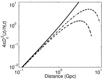
Figure 1: The dimensionless volume element per unit redshift, $\mathrm{d}V/\mathrm{d}z$ (cf Eq. (6) with $c=1=H_{0}$) as a function of comoving radial distance for the Euclidean, flat-$\Lambda$ (0.3, 0.7), and EdS cosmologies; $h(z)\equiv 1$ for the Euclidean case. Here we use shells of distance rather than shells of $z$ because redshift is inapplicable for the static Euclidean cosmology. The curves show that event counts in the flat-$\Lambda$ and EdS cosmologies reach a maximum and then decline. This is modified by source rate density evolution and, for event rates, by time dilation from cosmic expansion. For distances less than about 1 Gpc the curves converge to that of the Euclidean cosmology.

In a flat-$\Lambda$ cosmology, the density parameters of matter and vacuum energy sum to unity; we use $\Omega_{\mathrm{m}}=0.3$ and $\Omega_{\mathrm{\Lambda}}=0.7$ for their present-epoch values and take $H_{0}=70$ km s^-1 Mpc^-1 for the Hubble parameter at $z=0$. For comparison, we also consider the Einstein-de Sitter (EdS) cosmology—a flat Universe with zero vacuum energy—in which $\Omega_{\mathrm{m}}=1$ and $\Omega_{\mathrm{\Lambda}}=0$. Figure 1 plots $\mathrm{d}V/\mathrm{d}z$ as a function of comoving radial distance. It shows that volume elements (of fixed $\Delta z$) for the EdS and flat-$\Lambda$ cosmologies reach a maximum and then decline, a result of cosmic expansion.

2.3 Source rate density evolution

Neutron star (NS) births result from massive short-lived progenitor stars and there is mounting evidence that GRBs do so too, so both types of events should closely track the evolving star formation rate (SFR).

We use a dimensionless SFR density evolution factor $e(z)$, normalized to unity in our local intergalactic neighborhood, to account for source rate evolution:

$$e(z)=\frac{(1+W)e^{Qz}}{e^{Rz}+W}\;.$$ (7)

The two SFR models used in this paper have the parameter values

1. SF1: $(Q,R,W)=(3.4,3.8,45)$

2. SF2: $(Q,R,W)=(3.4,3.4,22)$

as fitted using the EdS cosmology with $H_{0}=65$ km s^-1 Mpc^-1 by Porciani & Madau (2001). The first star formation history matches most H$\alpha$ luminosity densities measured in the UV, and includes an upward correction for dust reddening. The second model includes more substantial dust extinction at high $z$.

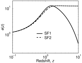
Figure 2: Dimensionless evolution factors, $e(z)$, normalized to unity at $z=0$, based on the parametrized star formation rate scenarios labelled as SF1 and SF2 in Porciani & Madau (2001) but scaled to the flat-$\Lambda$ (0.3, 0.7) cosmology; model SF2 allows for high dust extinction at high $z$.

An observation-based SFR density is cosmology-dependent, because it is deduced from the observed spectral luminosity in set volumes. The above SFR models can be re-scaled to other cosmologies, as shown in the appendix of Porciani & Madau (2001). The luminosity density, and hence SFR density, are proportional to ${D_{\mathrm{L}}}^{2}/(\mathrm{d}V/\mathrm{d}z)$, which is proportional to $(1+z)^{2}H(z)$, and so both scale as $H(z)$ among different cosmologies. But $e(z)$, which is normalized to unity at $z=0$, just follows the shape of the SFR density curve and so scales as $h(z)$; that is $e(z)/h(z)$ is invariant under change of cosmology. For converting the above evolution factors to a flat-$\Lambda$ cosmology with $\Omega_{\mathrm{m}}=0.3$ and $\Omega_{\Lambda}=0.7$, the scale factor is

$$[0.3(1+z)^{3}+0.7]^{1/2}(1+z)^{-3/2}\,,$$ (8)

as follows from Eq. (4) for $h(z)$. The resulting $e(z)$ functions are shown in Fig. 2.

2.4 PEH in flat-$\Lambda$ and EdS cosmologies

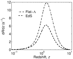
Figure 3: The differential neutron star birth rate, $\mathrm{d}R/\mathrm{d}z$, as a function of redshift, for the flat-$\Lambda$ (0.3, 0.7) and EdS cosmologies and the star formation rate model labelled SF1 in Porciani & Madau (2001) but scaled to the flat-$\Lambda$ (0.3, 0.7) cosmology. The present-epoch rate $r_{0}$ is taken to be $5\times 10^{-12}$ s^-1 Mpc^-3.

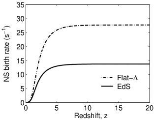
Figure 4: The cumulative neutron star birth rate, $R(z)$, obtained by integrating $\mathrm{d}R/\mathrm{d}z$ from $z=0$. Universal event rates (integrated throughout the cosmos) are 14 and 27 s^-1 in the EdS and flat-$\Lambda$ cosmologies respectively.

In the Euclidean model, the event rate in the shell $r$ to $r+{\mathrm{d}}r$ centred on the observer is $\mathrm{d}R=4\pi r^{2}r_{0}\mathrm{d}r$. In the standard Friedmann cosmologies, one can express the differential event rate as the event rate in the redshift shell $z$ to $z+{\mathrm{d}}z$:

$$\mathrm{d}R=\frac{\mathrm{d}V}{\mathrm{d}z}\frac{r_{0}e(z)}{1+z}\mathrm{d}z\,,$$ (9)

where $\mathrm{d}V$ is the cosmology-dependent co-moving volume element and $R(z)$ is the all-sky ($4\pi$ solid angle) event rate, as observed in our local frame, for sources out to redshift $z$. Source rate density evolution is accounted for by the dimensionless evolution factor $e(z)$; as this is normalized to unity in the present-epoch universe $(z=0)$, $r_{0}$ is now the $z=0$ rate density. The $(1+z)$ factor accounts for the time dilation of the observed rate by cosmic expansion, converting a source-count equation to an event rate equation.

The cumulative NS birth or GRB event rate $R(z)$ is calculated by integrating the differential rate from the present epoch to redshift $z$. It depends on cosmology through the factors $\mathrm{d}V/\mathrm{d}z$ and $e(z)$ in Eq. (9) for $\mathrm{d}R$. The differential and cumulative rates of NS formation as functions of $z$ are plotted in Figs. 3 and 4, for model SF1. Figure 4 shows that $R(z)$ is higher in the flat-$\Lambda$ (0.3, 0.7) cosmology than in the EdS one. Because the curves scale with $r_{0}$, they can also be applied to GRBs, but with the rates a factor of about $10^{6}$ lower for the classical GRBs.

For event types locked to the star formation rate, $e(z)$ is obtained by normalizing a SFR model to its $z=0$ value. Presently there is no consensus among astronomers on a model of star formation history at high $z$, so we shall use either a constant star formation history or the parametrized models of Porciani & Madau (2001).

Integrating the differential rate yields the cosmological analogue of the Euclidean mean cumulative event rate:

$$R(z)=\int_{0}^{z}(\mathrm{d}R/\mathrm{d}z)\;\mathrm{d}z\,.$$ (10)

Because of variation of cosmological volume elements (Fig.1), the rate derivative $\mathrm{d}R/\mathrm{d}z$ reaches a maximum at high $z$ in both the flat-$\Lambda$ and EdS cosmologies. Consequently there is a slower growth in the cumulative rate as compared to that in the simple Euclidean model in which the volume elements grow as $r^{2}$.

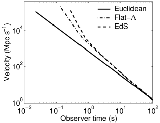
Figure 5: The probability event horizon (PEH) velocity for Euclidean, flat-$\Lambda$ (0.3, 0.7) and EdS cosmologies assuming a constant event rate density of $5\times 10^{-12}$ s^-1 Mpc^-3. The starting points at the upper left indicate that the PEH is ‘stalled’ until the number of events exceeds some threshold, which is cosmology dependent as a result of different cumulative event rate functions. The flat-$\Lambda$ and EdS curves depart markedly from the Euclidean curve during the first seconds of observation time. The change in gradient apparent in the flat-$\Lambda$ and EdS curves occurs because of a slower increase in volume at high $z$.

The events follow the same probability distribution as in the Euclidean case (Eq. 1) but with $R$ now expressed as a function of $z$:

$$p(n\geq 1;R(z),T)=1-e^{-R(z)T}=\epsilon\,,$$ (11)

with $N_{\epsilon}\equiv R(z)T=|\mathrm{ln}(1-\epsilon)|$ constant. Instead of inverting to find $r_{\epsilon}^{\mathrm{PEH}}(T)$, we find $z_{\epsilon}^{\mathrm{PEH}}(T)$ by solving this condition numerically, thus defining the PEH. Converting $z_{\epsilon}^{\mathrm{PEH}}(T)$ to luminosity distance and differentiating with respect to $T$ then yields $v_{\epsilon}^{\mathrm{PEH}}(T)$.

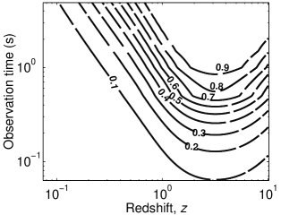
Figure 6: Contours, based on the same constant event rate density and flat-$\Lambda$ cosmology as used in Fig. 5, show the probability (labelling the curves) for at least one event to occur in the redshift shell $z$ to $z+\mathrm{d}z$ as a function of $z$ and observation time. The minimum of each of the contours corresponds to the most probable redshift at which an event will occur. As a function of observation time, each probability contour follows two trajectories — one approaching the observer and the other receding. The receding contours reach the redshift where events first started within a fraction of a second, as opposed to years in observer time for an approaching probability contour to reach the local Universe.

3 Neutron star birth events

Figure 5 shows the PEH velocity for NS birth events in the three cosmologies — Euclidean, flat-$\Lambda$ and EdS—with no source evolution so $e(z)=1$. Because the local Universe is approximately Euclidean, the PEH velocity converges to the Euclidean result when the observation time becomes much longer than the mean time interval between events. The cumulative rate, $R(z)$, is cosmology dependent, because the differential rate is determined by the evolution of volume elements as a function of $z$ (Eq. 6). Variations in event rates result in differing PEH velocities; for example, the relatively smaller event rate obtained using the EdS model (see Fig. 4) manifests as a longer time delay before the initiation of PEH motion because $p(n\geq 1;R(z),T)$ remains below 0.95 for a longer observation time.

Figure 6 shows probability contours, in the flat-$\Lambda$ cosmology, for at least one event to occur in the redshift shell $z$ to $z+{\mathrm{d}}z$ as a function of $T$ and $z$. The curves reveal two horizons, one approaching and one receding as $T$ increases; the receding horizon, corresponding to the observation of increasingly distant events beyond the peak of $\mathrm{d}R/\mathrm{d}z$, is very short lived.

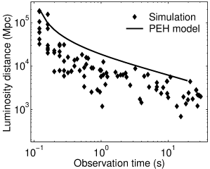
Figure 7: Simulation illustrating the rapid motion of the PEH for the first few tens of seconds of observation time, and a model curve with a probability threshold $\epsilon=0.95$ for at least one event to occur at a distance less than that of the PEH. We assume a universal cumulative event rate of about 25 s^-1 as seen in our frame, comparable to the NS birth rate integrated throughout the Universe, a flat-$\Lambda$ (0.3, 0.7) cosmology and a source rate evolution locked to the SFR model labelled SF2 in Porciani & Madau (2001)

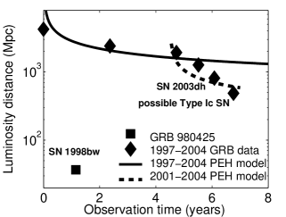
Figure 8: Filled diamonds show the closest events as a function of observation time for the 34 GRBs for which the redshift is known with reasonable confidence; the solid square is the highly under-luminous GRB 980425. The observations span a 7-yr period, starting from the first redshift measurement in 1997 February and continuing to 2004 July. The solid curve shows the PEH, excluding the outlier GRB980425, assuming a flat-$\Lambda$ (0.3, 0.7) cosmology and a source rate evolution based on the star formation rate model labelled SF1 in Porciani & Madau (2001). A local rate density $r_{0}\approx 0.8$ yr^-1 Gpc^-3 is used to fit to the redshift data for the classical GRBs for the first 4–5 yr of observation. (The probability of GRB 980425 occurring inside a volume bounded by its redshift $z=0.0085$ in this time is $5\times 10^{-5}$.) After this period, a more rapidly decreasing trend in distance is observed. The dashed curve shows the PEH model fitted to the data from 2001 September to 2004 July with $r_{0}\approx 27$ yr^-1 Gpc^-3. GRBs associated with core-collapse SNe are labelled.

To demonstrate the motion of a PEH we have simulated the occurrence, as a function of observation time, of NS birth events distributed throughout the Universe. The redshifts are treated as a random variable following a probability distribution function obtained by normalizing $dR/dz$ (Coward, Burman & Blair 2002a,b):

$$p(z){\mathrm{d}}z={\mathrm{d}}R/R(\infty)\;,$$ (12)

$R(\infty)$ being the Universal rate, integrated throughout the cosmos, as seen in our frame. The corresponding cumulative distribution function $C(z)$, giving the probability of an event occurring in the redshift range $0$ to $z$, is

$$C(z)=R(z)/R(\infty)\;.$$ (13)

We use the inverse function of $C(z)$ to produce values of $z$ by employing a random number generator to select values from $C(z)$.

Our simulation uses $r_{0}\approx 5\times 10^{-12}$ s^-1 Mpc^-3 for the $z=0$ rate density of these events and an evolution locked to the SFR model labelled SF2 in Porciani & Madau (2001) scaled to the flat-$\Lambda$ $(0.3,0.7)$ cosmology. The running minimum redshifts of the simulated events as a function of observation time define the PEH; these have been converted to luminosity distances and plotted in Fig. 7 along with a PEH curve for $\epsilon=0.95$. Of these 103 events only one is at a distance greater than the PEH. The binomial 95% confidence interval, give $0.9471<P<0.9998$ for one failure in 103 trials, which is in good agreement with $\epsilon=0.95$ for at least one event to occur within the PEH.

In this calculation of the approach of the PEH for simulated NS birth events throughout the Universe, we have assumed that the observation time for each event is small compared with the typical observed temporal separation of events, which averages about 40 ms. The calculation is directed toward future ‘Advanced LIGO’-type gravitational wave detectors, which may be able to detect a stochastic background of gravitational radiation generated by these events. Recent calculations, based on the computed wave functions of Dimmelmeier, Font & Müller (2002), suggest that the duty cycle of the signal will be well below one (Howell et al., 2004, figure 16), implying a signal consisting largely of non-overlapping wave-trains, described as ‘popcorn noise’.

For optical surveys of very high-$z$ SNe, selection effects and the sensitivity limits of the detectors reduce the observed rate substantially. If these effects were well enough understood, then the rate density of events could still be inferred from the evolving record of observations. These ideas will be demonstrated in the next section for GRB afterglow observations.

Table 1: GRB redshifts adapted from the table of localized GRBs at http://www.aip.de/$\sim$jcg/grbgen.html. The instruments used to localize the GRBs are listed along with confirmation if the Interplanetary Network (IPN) was used. Other columns show: XA = X-ray afterglow; OT = optical (or IR) transient; RA = radio afterglow; IAUC (International Astronomical Union Circular) number; $z$ = redshift. An ‘X’ after the date marks events with no gamma-ray detection, but with X-ray properties similar to GRBs – so-called X-ray flashes. The ‘C’ after one of the dates identifies it as the 3rd GRB on that day. The running minimum observed GRB redshifts from 1997 February to 2004 July (entries highlighted in bold) are used in Fig. 8, with GRB 980425 regarded as an outlier.

GRB	Instrument	IPN	XA	OT	RA	IAUC	$z$
970228	SAX/WFC	y	y	y	n	6572	0.695
970508	SAX/WFC		y	y	y	6649, 6654	0.835
970828	SAX/WFC	y	y	n	y	6726, 6728	0.9578
971214	SAX/WFC	y	y	y	n	6787, 6789	3.42
980425	SAX/WFC		y	SN	y	6884	0.0085
980613	SAX/WFC		y	y	n	6938	1.096
980703	RXTE/ASM		y	y	y	6966	0.966
990123	SAX/WFC	y	y	y	y	7095	1.6
990506	BAT/PCA	y	y		y	-	1.3
990510	SAX/WFC	y	y	y	y	7160	1.619
990705	SAX/WFC	y	y	y	n	7218	0.86
990712	SAX/WFC			y	n	7221	0.434
991208	Uly/KO/NE	y		y	y		0.706
000131	Uly/KO/NE	y		y			4.5
000210	SAX/WFC	y	y		y		0.846
000301C	ASM/Uly	y		y	y		2.03
000911	Uly/KO/NE	y		y	y		1.058
000926	Uly/KO/NE	y	y	y	y		2.066
010921	HE/Uly/SAX	y		y			0.45
011121	SAX/WFC	y	y	y	y		0.36
011211	SAX/WFC		y	y			2.14
020124	HETE	y		y			3.198
020405	Uly/MO/SAX	y		y	y		0.69
020813	HETE	y	y	y	y		1.25
020903X	HETE			y	y		0.25
021004	HETE		y	y	y		2.3
021211	HETE			y			1.01
030226	HETE		y	y			1.98
030323	HETE				y		3.372
030328	HETE		y	y			1.52
030329	HETE		y	y	y	8101	0.168
030429	HETE			y			2.65
031203	INTEGRAL		y	y	y	8250, 8308	0.105
040701X	HETE		y				0.2146

4 GRB events

The PEH velocity is based on the act of observation, where the observer is at the centre of a Universe defined in terms of an event probability distribution. The temporal evolution of the PEH for a particular class of cosmological transient event is defined by the history of event rates. Different types of events, for example NS births and GRBs, will have different PEH velocities because their mean event rate densities differ, even if both are locked to the SFR. The PEH concept can be applied to the observed GRB redshift distribution assuming some knowledge of source-rate evolution, luminosity distribution of the sources, observational selection effects and the local rate density; these parameters are all uncertain.

We use GRB redshift data from 1997 Febuary (when the first GRB redshift was obtained) to 2004 July, which consist of 235 GRBs localized to less than 1 degree within a few hours to days. About 40 GRB redshifts have been measured but only 34 are known with certainty (mostly identified from their host galaxies); these events, along with details of each observation, are shown in Table 1.

Figure 8 plots the temporal evolution of the minimum observed luminosity distance, using these measured GRB redshifts, as a function of observation time from 1997 February to 2004 July; we do not include GRB redshifts that are highly uncertain. We note that the very under-luminous and nearby GRB 980425 ($z=0.0085$ corresponding to 40 Mpc), and GRBs 030329 $(z=0.168)$ and 031203 $(z=0.105)$, are associated with cc SNe, probably Type Ib/c.

Our data points are obtained by selecting the sources with minimum redshift as a function of observation time over the GRB redshift data set. A PEH model curve is fitted to these data, assuming the flat-$\Lambda$ (0.3, 0.7) cosmology and a source rate evolution locked to the SFR model labelled SF1 in Porciani & Madau (2001). The differential rate has one free parameter, the present-epoch GRB rate density, $r_{0}$, which we vary in the PEH model to fit the data. We scale the differential event rate by a GRB luminosity function following a log-normal distribution (Bromm & Loeb, 2002), with a mean GRB luminosity of $2\times 10^{56}$ photons s^-1, and assume a photon flux threshold of 0.2 s^-1 cm^-2 for BATSE (see Appendix A). We note that the form of luminosity distribution that would fit both the ‘classical’ GRBs and GRBs 980425 and 031203 is not apparent.

Excluding the outlier GRB 980425, we find that the data for the first 4–5 yr of observation time (classical GRBs) are best fitted using a PEH curve with $r_{0}\approx 6\times 10^{-2}$ yr^-1 Gpc^-3. Scaling this rate by accounting for the solid angle monitored by the BeppoSAX camera or HETE telescope, about 0.9 str (Guetta, 2004), yields $r_{0}\approx 0.8$ yr^-1 Gpc^-3, similar to the rate density of 0.5 yr^-1 Gpc^-3 deduced from observations of both optical and optically dark GRBs (Schmidt, 2001; Frail et al., 2001). The probability of at least one GRB occurring inside a volume bounded by $z=0.17$ (in 4.5 yrs observation time) has the quite significant value of 0.37, but the probability of one occurring inside a volume bounded by $z=0.0085$ is only about $5\times 10^{-5}$: it is difficult to reconcile the very nearby GRB 980425 with the redshift distribution of classical GRBs. Soderberg et al. (2004) conclude that the two under-luminous GRBs 980425 and 031203 were intrinsically sub-energetic and un-jetted events.

Data from 2001–2004, which include GRBs 030329 and 031203, show a more sharply decreasing trend in Fig. 8, implying a relatively higher PEH velocity and so a higher $R(z)$ and hence a higher $r_{0}$; fitting a PEH curve to this subset of data requires $r_{0}\approx 27$ yr^-1 Gpc^-3. With this $r_{0}$, the probability for an event to occur in the volume bounded by GRB 980425 $(z=0.0085)$ in 4.5 yr is 0.0016. Thus, it seems likely that GRB 980425 is a member of a more numerous population of low-luminosity GRBs.

Because GRBs 980425 and 031203 were sub-energetic and showed no evidence for jetted emissions, $r_{0}$ for such a low-luminosity GRB population could be orders of magnitude higher than that of the classical GRB population, but still only a small fraction of the Type Ib/c SN rate (Coward, 2005).

5 Concluding remarks

The probability event horizon concept provides a means of analyzing an observer’s evolving record of events in terms of the distribution of the sources throughout the cosmos. It is particularly sensitive to the shape of the low probability ‘tail’ of the source distribution. The dependence of the PEH velocity on the local source rate density means that by analyzing the redshift distribution of the sources as a function of observation time one can infer the local source rate density.

As an initial application of this, we have shown how fitting a PEH model to GRB redshift data can yield information on the local GRB rate density. Such an analysis can be used to probe the progenitor populations that comprise the distributions. This is demonstrated by Figure 8, where GRB 980425 is either a statistical outlier of the classical population or a member of a different distribution of GRBs that could be intrinsically faint; alternatively, it could be a classical GRB observed away from its jet axis.

The PEH concept has applications to gravitational wave detection. Understanding the detectability of astrophysical sources as a function observation time is crucial to these searches. Current detectors are only sensitive to local events, such as binary coalescences out to several tens of Mpc; the PEH for these events corresponds to long observation times of the order of a year or so. Because of the rarity of such events, we are modelling the detectability of more frequent but fainter gravitational wave sources using the PEH concept.

We are currently studying the application of the PEH in simulations of the evolving spectra of contributions to the stochastic gravitational wave background generated by NS births and other cataclysmic events distributed throughout the Universe.

Appendix A GRB Luminosity function

The GRB luminosity function (LF), together with the flux sensitivity threshold of the instrument, determines the fraction of all GRBs potentially detectable with that instrument (Norris, 2002). Following Bromm & Loeb (2002), we scale $\mathrm{d}R/\mathrm{d}z$ to account for the distribution of GRB luminosities:

$$\psi_{\rm GRB}(z)=\int_{L_{\rm lim}(z)}^{\infty}p(L){\rm d}L\;,$$ (14)

where $\psi_{\rm GRB}(z)$ is the GRB rate scaling function and $p(L)$ is the GRB LF with $L$ the intrinsic luminosity in units of photons s^-1. With $f_{\rm lim}$ denoting the flux sensitivity threshold, in photons s^-1 m^-2, the minimum detectable luminosity can be expressed as a function of redshift by $L_{\rm lim}(z)=4\pi{D_{\mathrm{L}}}^{2}(z)f_{\rm lim}$, with $D_{\mathrm{L}}(z)$ the luminosity distance.

In modelling the GRB redshift distribution we use the log-normal LF cited by Bromm & Loeb (2002):

$$p(L)=\frac{{\rm e}^{-\sigma^{2}/2}}{\sqrt{2\pi\sigma^{2}}}\exp\bigg{\{}-\frac{[\ln(L/L_{0})]^{2}}{2\sigma^{2}}\bigg{\}}\frac{1}{L_{0}}\;,$$ (15)

where $\sigma$ and $L_{0}$ are the width and average luminosity, respectively. We assume $\sigma=2$ and $L_{0}=2\times 10^{56}$ s^-1, with $f_{\rm lim}=0.2$ photons s^-1 cm^-2 for BATSE (Bromm & Loeb, 2002).

References

- Barris et al. (2004) Barris B.J. et al., 2004, ApJ, 602, 571
- Bromm & Loeb (2002) Bromm V., Loeb A., 2002, ApJ, 575, 111
- Coward, Burman & Blair (2001) Coward D.M., Burman R.R., Blair D.G., 2001, MNRAS, 324, 1015
- Coward, Burman & Blair (2002) Coward D.M., Burman R.R., Blair D.G., 2002a, MNRAS, Soc. 329, 411
- Coward, Burman & Blair (2002) Coward D., Burman R., Blair D., 2002b, Class. Quantum Grav. 19, 1303
- Coward (2005) Coward D.M., MNRAS, 2005 (submitted)
- Dimmelmeier, Font & Müller (2002) Dimmelmeier H., Font, J.A., Müller, E., 2002, A&A, 393, 523
- Frail et al. (2001) Frail D.A. et al., 2001, ApJ, 562, L55
- Guetta (2004) Guetta D., Perna R., Stella L., Vietri M., 2004, ApJ, 615, L73
- Hogg (2000) Hogg D.W., 2000, astro-ph/9905116 v4
- (11) Howell E., Coward D., Burman R., Blair D., MNRAS, 2004, 351, 1237
- Norris (2002) Norris J.P., 2002, ApJ, 579, 386
- Peebles (1993) Peebles P.J.E., 1993, Principles of Physical Cosmology, Princeton Univ. Press, Princeton, New Jersey, p. 312
- Porciani & Madau (2001) Porciani C., Madau P., 2001, ApJ., 548, 522
- Schmidt (2001) Schmidt M., 2001, ApJ, 552, 36
- Soderberg et al. (2004) Soderberg A.M. et al., 2004, Nat., 430, 648
- van Putten & Regimbau (2004) van Putten M.H.P.M., Regimbau T., 2003, ApJ, 593, L15