Self-similar solutions for relativistic shocks
emerging from stars with polytropic envelopes

Abstract

We consider a strong ultrarelativistic shock moving through a star whose envelope has a polytrope-like density profile. When the shock is close to the star’s outer boundary, its behavior follows the self-similar solution given by Sari (2005) for implosions in planar geometry. Here we outline this solution and find the asymptotic solution as the shock reaches the star’s edge. We then show that the motion after the shock breaks out of the star is described by a self-similar solution remarkably like the solution for the motion inside the star. In particular, the characteristic Lorentz factor, pressure, and density vary with time according to the same power laws both before and after the shock breaks out of the star. After emergence from the star, however, the self-similar solution’s characteristic position corresponds to a point behind the leading edge of the flow rather than at the shock front, and the relevant range of values for the similarity variable changes. Our numerical integrations agree well with the analytic results both before and after the shock reaches the star’s edge.

1 Introduction

The surge of activity over the past decade or so in the fields of supernovae and of gamma-ray bursts and their afterglows has led to renewed investigation into the behavior of strong shocks. Much of the analytic work on strong shock propagation to date has focused on self-similar solutions to the hydrodynamic equations. In these solutions, the profiles of the hydrodynamic variables as functions of position have constant overall shapes whose time evolution consists simply of scalings in amplitude and position. As a result, self-similarity allows us to reduce the nominal system of two-dimensional partial differential hydrodynamic equations to a system of one-dimensional ordinary differential equations. The existence of self-similar solutions thus enables a significant simplification of problems free of spatial scales in regions far from the initial conditions. The best-known such solutions are the pioneering Sedov-Taylor solutions for non-relativistic point explosions propagating into surroundings with power-law density profiles (Sedov, 1946; von Neumann, 1947; Taylor, 1950).

Self-similar solutions are traditionally divided into two categories (see, for example, Zel’dovich & Raizer (1967) for a detailed discussion). ‘Type I’ solutions are those in which the time evolution of the shock position and hydrodynamic variables follows from global conservation laws such as energy conservation. The Sedov-Taylor solutions are Type I; their ultrarelativistic analogues were found by Blandford & McKee (1976). By contrast, global conservation laws are useless in ‘Type II’ solutions, which are instead characterized by the requirement that the solution remain well-behaved at a singular point known as the ‘sonic point’. If, for instance, the density of the surroundings falls off very quickly with distance, Type II solutions found by Waxman & Shvarts (1993) for non-relativistic spherical explosions hold instead of the Sedov-Taylor solutions and relativistic solutions found by Best & Sari (2000) hold instead of the Blandford-McKee solutions.

Here we study the case of an ultrarelativistic shock wave moving outwards through a star whose envelope has a polytrope-like density profile. After the shock front reaches the outer edge of the star, an event we refer to as ‘breakout’, the shock front itself ceases to exist but the shocked fluid continues outward into the vacuum originally surrounding the star. We focus on the flow at times just before and just after breakout. As explained in §2, the shock evolution just inside the star’s surface is identical to that expected for an imploding planar shock in a medium with a power-law density profile. Such a shock follows a Type II self-similar solution as discussed by Sari (2005) and Nakayama & Shigeyama (2005) and outlined briefly here. §3 describes the asymptotic solution as the shock front reaches the surface of the star, a singular point. In §4 we investigate the flow after breakout. We show that the self-similar solution for the evolution inside the star also describes the behavior outside the star except in that a different range of the similarity variable applies and in that the physical interpretation of the characteristic position changes. We show in §5 that the analytic results of §2, 3, 4 agree with our numerical integrations of the relativistic time-dependent hydrodynamic equations, and in §6 we summarize our findings. Throughout our discussion, we take the speed of light to be $c=1$.

2 Shock propagation within the star

Since we are interested in the shock after it has reached the envelope or the outermost layers of a star, we assume that the mass and distance lying between the shock front and the star’s outer edge are much less than the mass and distance between the shock front and the star’s center. In this region, we can take the star’s gravity $g$ to be constant and the geometry to be planar. We also assume that the stellar envelope has a polytrope-like equation of state, that is, $p\propto\rho^{q}$ where $p$ is the pressure, $\rho$ is the mass density, and $q$ is a constant. This type of equation of state occurs in various contexts including fully convective stellar envelopes, in which case $q$ is the adiabatic index; radiative envelopes where the opacity has a power-law dependence on the density and temperature; and degenerate envelopes.

Under these assumptions we can find the density profile from hydrostatic equilibrium and the equation of state as follows. Let $x$ be the radial coordinate such that $x=0$ at the star’s surface and $x<0$ inside the star. Then

$$0=\frac{dp}{dx}+\rho g$$ (1)

and with the boundary condition $\rho=p=0$ at the edge of the star, we have

$$\frac{q}{q-1}\rho^{q-1}\propto-gx$$ (2)

$$\rho\propto(-x)^{1/(q-1)}=(-x)^{-k}\;\;\;.$$ (3)

For convective and degenerate envelopes, $q$ is between $4/3$ and $5/3$; for radiative envelopes with Kramers opacity, $q=30/17$. These give $k$ values between $-1$ and $-3$.

With the power-law density profile $\rho\propto(-x)^{-k}$, the evolution of an ultrarelativistic shock propagating through the envelope is given by a Type II converging planar self-similar solution to the hydrodynamic equations representing energy, momentum, and mass conservation,

$$\frac{\partial}{\partial t}\left[\gamma^{2}(e+\beta^{2}p)\right]+\frac{\partial}{\partial x}\left[\gamma^{2}\beta(e+p)\right]=0$$ (4)

$$\frac{\partial}{\partial t}\left[\gamma^{2}\beta(e+p)\right]+\frac{\partial}{\partial x}\left[\gamma^{2}(\beta^{2}e+p)\right]=0$$ (5)

$$\frac{\partial}{\partial t}(\gamma n)+\frac{\partial}{\partial x}(\gamma\beta n)=0\;\;\;,$$ (6)

with the ultrarelativistic equation of state

$$p=\frac{1}{3}e\;\;\;.$$ (7)

Here we will simply state the solution; for a detailed derivation see Sari (2005) or Nakayama & Shigeyama (2005). We assume the effect of the star’s gravity on the shock propagation is negligible. Following Sari (2005), we let $R(t)$ be the solution’s characteristic position, which we choose to be the position of the shock front while the shock is within the star. We take $t=0$ at the time the shock reaches the star’s surface ($R=0$), and we take $R<0$ when $t<0$. We take $\Gamma(t)$, $P(t)$, and $N(t)$ to be respectively the characteristic Lorentz factor, pressure, and number density, and we define

$$\frac{t\dot{\Gamma}}{\Gamma}=-\frac{m}{2}\;\;\;,\;\;\;\frac{t\dot{P}}{P}=-m-k\;\;\;,\;\;\;\frac{t\dot{N}}{N}=-\frac{m}{2}-k\;\;\;.$$ (8)

Following Blandford & McKee (1976), we define the similarity variable as

$$\chi=1+2(m+1)\frac{R-x}{R/\Gamma^{2}}\;\;\;.$$ (9)

Note that for $R<0$, $x\leq R$ and the relevant range in $\chi$ is $-\infty<\chi<1$ as long as $m>-1$. We define the hydrodynamic variables—the Lorentz factor $\gamma$, the pressure $p$, and the number density $n$—as follows:

$$\gamma^{2}(x,t)=\frac{1}{2}\Gamma^{2}(t)g(\chi)$$ (10)

$$p(x,t)=P(t)f(\chi)$$ (11)

$$n(x,t)=N(t)\frac{h(\chi)}{g^{1/2}(\chi)}\;\;\;.$$ (12)

Here $g$, $f$, and $h$ give the profiles of $\gamma$, $p$, and $n$; expressions for the dependence of $m$ on $k$ and for $g$, $f$, $h$ as functions of $\chi$ make up the entire self-similar solution. The above definitions and the ultrarelativistic hydrodynamic equations in planar geometry put the sonic point, the point separating fluid elements which can communicate with the shock front via sound waves from those which cannot, at $g\chi=4-2\sqrt{3}$. Requiring that the solution pass smoothly through this point gives

$$m=\left(3-2\sqrt{3}\right)k$$ (13)

$$g=C_{g}\left|\frac{g\chi}{3k-2k\sqrt{3}+1}-2(2+\sqrt{3})\right|^{-\left(3-2\sqrt{3}\right)k}$$ (14)

$$f=C_{f}\left|-g\chi-2k\sqrt{3}+4+2\sqrt{3}\right|^{-\left(4-2\sqrt{3}\right)k}$$ (15)

$$h=C_{h}\left|g\chi+2k\sqrt{3}-4-2\sqrt{3}\right|^{-\frac{\left(2\sqrt{3}-3\right)(2k-1)k}{(-1+k\sqrt{3}-\sqrt{3})}}|g\chi-2|^{\frac{k}{-1+k\sqrt{3}-\sqrt{3}}}\;\;\;.$$ (16)

The boundary conditions $g(\chi=1)=f(\chi=1)=h(\chi=1)=1$ which hold inside the star allow us to determine the constants of integration $C_{g}$, $C_{f}$, $C_{h}$ and write

$$g=\left[\frac{-g\chi-2k\sqrt{3}+4+2\sqrt{3}}{-1-2k\sqrt{3}+4+2\sqrt{3}}\right]^{-\left(3-2\sqrt{3}\right)k}$$ (17)

$$f=\left[\frac{-g\chi-2k\sqrt{3}+4+2\sqrt{3}}{-1-2k\sqrt{3}+4+2\sqrt{3}}\right]^{-(4-2\sqrt{3})k}$$ (18)

$$h=\left[\frac{g\chi+2k\sqrt{3}-4-2\sqrt{3}}{1+2k\sqrt{3}-4-2\sqrt{3}}\right]^{-\frac{\left(2\sqrt{3}-3\right)(2k-1)k}{-1+k\sqrt{3}-\sqrt{3}}}\left[2-g\chi\right]^{\frac{k}{-1+k\sqrt{3}-\sqrt{3}}}\;\;\;.$$ (19)

3 Transition at breakout

To know what happens to the shocked material after the shock front emerges from the star, we need the behavior of the shock just as the front reaches the surface—the ‘initial conditions’ for the evolution of the shock after breakout. Specifically, we are interested in the limiting behavior of each fluid element and in the asymptotic profiles of $\gamma$, $p$, and $n$ as functions of $x$ as $t$ and $R$ approach 0.

The limiting behavior of a given fluid element may be found as follows. Due to the self-similarity, we know the time taken for $\gamma$, $p$, and $n$ of a given fluid element to change significantly is the timescale on which $R$ changes by an amount of order itself. Since $R$ can change by this much only once between the time a given fluid element is shocked and the time the shock breaks out of the star, the limiting values of $\gamma$, $p$, and $n$ for that fluid element should be larger only by a factor of order unity from their values when the fluid element was first shocked.

We can also find the scalings of $\gamma$, $p$, and $n$ with $x$ at breakout via simple physical arguments. We denote by $x_{0}$, $\gamma_{0}$, $p_{0}$, $n_{0}$ the position, Lorentz factor, pressure, and number density of a fluid element just after being shocked and by $x_{f}$, $\gamma_{f}$, $p_{f}$, $n_{f}$ those values at the time the shock breaks out. Since the shock accelerates to infinite Lorentz factors, and since, as we found above, the Lorentz factor of a given fluid element remains constant up to a numerical factor, this fluid element will lag behind the shock by $x_{f}\sim x_{0}/\gamma_{0}^{2}$ at $t=0$. Eq. 8 gives $\Gamma\sim t^{-m/2}$, so we have $\gamma_{0}\sim(-x_{0})^{-m/2}$; then $\gamma_{f}\sim((-x_{f})\gamma_{f}^{2})^{-m/2}$ or

$$\gamma_{f}\sim(-x_{f})^{-m/2(m+1)}\;\;\;.$$ (20)

Likewise, since $P\sim t^{-m-k}$ and $N\sim t^{-m/2-k}$, we have $p_{0}\sim x_{0}^{-m-k}$ and $n_{0}\sim x_{0}^{-m/2-k}$; then

$$p_{f}\sim((-x_{f})\gamma_{f}^{2})^{-m-k}\sim(-x_{f})^{-(m+k)/(m+1)}$$ (21)

$$n_{f}\sim(-x_{f})^{-(m/2+k)/(m+1)}\;\;\;.$$ (22)

We can use the equations for the solution before breakout to perform equivalent calculations of the limiting behavior of fluid elements and asymptotic profiles of $\gamma$, $p$, $n$. For the limiting behavior of a fluid element, we take the advective time derivative of $g\chi$ and use the result to relate $\gamma$ and $g$ to time for that fluid element. The advective derivative is given by

$$\frac{D}{Dt}=\frac{\partial}{\partial t}+\beta\frac{\partial}{\partial r}=\dot{\Gamma}\frac{\partial}{\partial\Gamma}+\dot{P}\frac{\partial}{\partial P}+\frac{m+1}{t}(2/g-\chi)\frac{\partial}{\partial\chi}\;\;\;.$$ (23)

We apply this derivative to Eq. 17 to get

$$\frac{D(g\chi)}{D\log t}=\frac{(2-g\chi)\left(g\chi-4-2\sqrt{3}+2\sqrt{3}k\right)}{\left(g\chi-4-2\sqrt{3}\right)}$$ (24)

and integrate to get

$$t/t_{0}=\left|g\chi-2\right|^{(3+\sqrt{3})/(3k-\sqrt{3}-3)}\left|\frac{g\chi-4-2\sqrt{3}+2k\sqrt{3}}{1-4-2\sqrt{3}+2k\sqrt{3}}\right|^{-3k/\left(-\sqrt{3}-3+3k\right)}$$ (25)

where $t_{0}$ is the time at which the fluid element is shocked, that is, when $g=\chi=1$. When $\left|g\chi\right|\gg 1$—which becomes true everywhere behind the shock front as $t\rightarrow 0$—this simplifies to

$$t/t_{0}\simeq\left|g\chi\right|^{-1}\left|1-4-2\sqrt{3}+2k\sqrt{3}\right|^{3k/\left(-\sqrt{3}-3+3k\right)}$$ (26)

and Eq. 17 simplifies to

$$g\simeq\left[\frac{-g\chi}{-1-2k\sqrt{3}+4+2\sqrt{3}}\right]^{-\left(3-2\sqrt{3}\right)k}\;\;\;.$$ (27)

We substitute Eq. 26 into Eq. 27 to get the limiting Lorentz factor of the fluid element as $t\rightarrow 0$:

$$\gamma=\gamma_{0}\left|1-4-2\sqrt{3}+2k\sqrt{3}\right|^{-\left(3-3\sqrt{3}\right)k/\left(2\left(-\sqrt{3}-3+3k\right)\right)}$$ (28)

which is greater only by a numerical factor than the initial Lorentz factor $\gamma_{0}$ that the fluid element received right after being shocked. To relate the limiting $p$, $n$ to $p_{0}$, $n_{0}$, we likewise take Eqs. 18, 19 in the limit $|g\chi|\gg 1$ and use Eqs. 26, 27 with the results to get

$$p=p_{0}\left|1-4-2\sqrt{3}+2k\sqrt{3}\right|^{-\left(6-2\sqrt{3}\right)k/\left(-\sqrt{3}-3+3k\right)}$$ (29)

$$n=n_{0}\left|1-4-2\sqrt{3}+2k\sqrt{3}\right|^{-\frac{\left(4k+k\sqrt{3}-3-\sqrt{3}\right)\left(3-2\sqrt{3}\right)k}{2\left(k\sqrt{3}-1-\sqrt{3}\right)}}$$ (30)

which again differ only by numerical factors from their values just after the fluid element is shocked. This is consistent with the behavior given above by simple physical considerations.

For the analogous calculation of the asymptotic profiles of $\gamma$, $p$, and $n$, we cannot simply apply Eqs. 10, 11, 12: Eqs. 8, 9 require that $\chi\rightarrow-\infty$ everywhere behind the shock and $\Gamma$, $P$, and $N$ diverge as $t\rightarrow 0$. Instead we take the $t\rightarrow 0$ limit at a fixed position $x$. First we have

$$\chi=1+2(m+1)(1-x/R)\Gamma^{2}\simeq 2(m+1)(-x/R)\Gamma^{2}\;\;\;.$$ (31)

With Eqs. 10, 27 this gives

$$2\gamma^{2}/\Gamma^{2}=g=\left[\frac{-4(m+1)(-x)\gamma^{2}/R}{-1-2k\sqrt{3}+4+2\sqrt{3}}\right]^{-m}$$ (32)

and

$$\gamma=\left[2\frac{(-R)^{-m}}{\Gamma^{2}}\right]^{-1/2(1+m)}\left[\frac{4(m+1)}{-1-2k\sqrt{3}+4+2\sqrt{3}}\right]^{-m/2(1+m)}(-x)^{-m/2(1+m)}\;\;\;.$$ (33)

This is consistent with our qualitative discussion; the coefficient in the qualitative relation is a numerical factor times the constant $(-R)^{-m}/\Gamma^{2}$. For the $p$ and $n$ profiles, we apply a similar analysis to the expressions for $f$ and $h$ in the limit $t\rightarrow 0$.

$$p=P\left[2\frac{(-R)}{\Gamma^{2}}\right]^{\frac{m+k}{1+m}}\left[\frac{4(m+1)}{-1-2k\sqrt{3}+4+2\sqrt{3}}\right]^{-\frac{m+k}{1+m}}(-x)^{-\frac{m+k}{1+m}}$$ (34)

$$n=N\left[2\frac{(-R)}{\Gamma^{2}}\right]^{\frac{m/2+k}{1+m}}\left[4(m+1)\right]^{-\frac{m/2+k}{1+m}}\left[-1-2k\sqrt{3}+4+2\sqrt{3}\right]^{\frac{m/2+k}{1+m}+\frac{k}{-1+k\sqrt{3}-\sqrt{3}}}(-x)^{-\frac{m/2+k}{1+m}}$$ (35)

These results are likewise consistent with our qualitative discussion.

4 Evolution after breakout

4.1 Self-similar solution

Since the breakout itself does not introduce new spatial scales into the flow, we expect the motion after breakout to remain self-similar. However, as the shock Lorentz factor diverges at $t=0$, we cannot continue to associate the characteristic position, Lorentz factor, pressure, and number density with the values at the shock front after breakout. So we begin by providing physical motivation for a different characteristic Lorentz factor and exploring the implications of this choice.

We note that after breakout each fluid element expands and accelerates over time until the element’s internal energy has been converted entirely into bulk motion. Given a relativistic strong shock, the internal energy of a shocked fluid element in the frame moving with the fluid is comparable to the bulk kinetic energy of the fluid element. This implies that the fluid element’s final bulk Lorentz factor should be much greater than the value of the shock Lorentz factor just after the fluid element was shocked. The timescale $t_{x}$ for the resulting expansion and acceleration is the time over which the fluid element’s size and Lorentz factor change by a factor of order unity. For a fluid element located at $-x$ and with Lorentz factor $\gamma_{x}$ at $t=0$, the time of breakout, this timescale is $t_{x}=x\gamma_{x}^{2}$ due to relativistic beaming. That every time $t>0$ is thus associated in a scale-independent way with a particular $t_{x}$ and $\gamma$ suggests that we pick $\Gamma(t=t_{x})=\gamma_{x}$ to be the characteristic Lorentz factor.

To see how $\Gamma$ evolves with time, we use $\gamma\propto(-x)^{-m/2(1+m)}$ from Eq. 33 with the $t_{x}$ relation above to get $\Gamma\propto t^{-m/2}$. For the characteristic pressure $P$ and number density $N$, Eqs. 34, 35 likewise give $P\propto t^{-m-k}$ and $N\propto t^{-m/2-k}$. In other words, Eq. 8 holds after breakout with exactly the same $k$, $m$ that apply inside the star. The characteristic position $R$ is again the position which evolves according to the Lorentz factor $\Gamma$: $\dot{R}\simeq 1-1/2\Gamma^{2}$. Since the hydrodynamic equations still hold as well, Eqs. 9, 14, 15, 16 must remain valid when $t>0$.

To find the complete solution after breakout we need to specify the boundary conditions. We proceed by looking at the behavior of the similarity variables $\chi$, $g$, $f$, $h$. The relevant range in $\chi$ depends on $R$, and while the relation between $R$ and $\Gamma$ is the same before and after breakout, $R$ after breakout is not the position of the shock front. Instead, the front has infinite Lorentz factor and $R$ lags further and further behind the shock with increasing time. A nice physical interpretation exists for $R$ after breakout. $R$ tracks the position corresponding to a fluid element which has expanded by a factor of order unity, so $R$ marks the transition in position between fluid elements which have expanded and accelerated significantly since being shocked and fluid elements whose size and speed have remained roughly constant. Since it takes longer for fluid elements with smaller Lorentz factors to expand and accelerate significantly, $R$ moves backward relative to the leading edge of the flow at $x=t$. Because $R$ becomes positive after breakout, the range of possible $x$ in the solution outside the star is $x\leq t$. Then $\chi=0$ at the ‘front’ $x=t$, and the relevant range in $\chi$ in the solution outside is $0<\chi<\infty$ rather than $-\infty<\chi<1$.

Far behind $x=t$, the profiles of $\gamma$, $p$, and $n$ before breakout must coincide with the profiles after breakout. We know this because at a given time after breakout, sound waves carrying the information that breakout occurred can only have traveled a finite distance behind the shock front; material further behind continues to flow as if the breakout had never occurred. Also, the two sets of profiles must coincide at $t=0$, when everything is far behind the front. To phrase this requirement on the profiles in terms of the similarity variable, $g(\chi\rightarrow-\infty)$, $f(\chi\rightarrow-\infty)$, and $h(\chi\rightarrow-\infty)$ before breakout must coincide with $g(\chi\rightarrow\infty)$, $f(\chi\rightarrow\infty)$, and $h(\chi\rightarrow\infty)$ after breakout. Then as $\chi\rightarrow\infty$ after breakout, $g,f,h\rightarrow 0$ and $g\chi\rightarrow\infty$. In addition, the constants $C_{g}$, $C_{f}$, $C_{h}$ in Eqs. 14, 15, 16 must be the same for both the pre- and post-breakout solutions. In other words, the solutions before and after breakout, as specified by Eqs. 9, 14, 15, 16 and expressions for $C_{g}$, $C_{f}$, $C_{h}$, are the same; only the relevant ranges in $\chi$ and the physical interpretations of the variables differ. So the expressions for $g$, $f$, $h$ after breakout are

$$g=\left[\frac{g\chi+2k\sqrt{3}-4-2\sqrt{3}}{-1-2k\sqrt{3}+4+2\sqrt{3}}\right]^{-\left(3-2\sqrt{3}\right)k}$$ (36)

$$f=\left[\frac{g\chi+2k\sqrt{3}-4-2\sqrt{3}}{-1-2k\sqrt{3}+4+2\sqrt{3}}\right]^{-(4-2\sqrt{3})k}$$ (37)

$$h=\left[\frac{-g\chi-2k\sqrt{3}+4+2\sqrt{3}}{1+2k\sqrt{3}-4-2\sqrt{3}}\right]^{-\frac{\left(2\sqrt{3}-3\right)(2k-1)k}{-1+k\sqrt{3}-\sqrt{3}}}\left[g\chi-2\right]^{\frac{k}{-1+k\sqrt{3}-\sqrt{3}}}\;\;\;.$$ (38)

The boundary conditions after breakout are given explicitly by $g=f=1$ and $h=\left(5+4\sqrt{3}-4\sqrt{3}k\right)^{k/\left(-1-\sqrt{3}+k\sqrt{3}\right)}$ at $\chi=7+4\sqrt{3}-4\sqrt{3}k$. A graphical comparison between the pre- and post-breakout $\gamma$ vs. position profiles is given in Figure 1 along with sample trajectories of fluid elements.

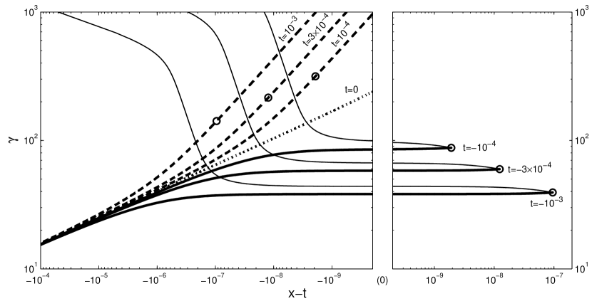
Figure 1: Profiles of $\gamma$ as a function of position (heavy lines) at seven different times marked on the figure and trajectories of three fluid elements in position-Lorentz factor space (thin lines). Fluid elements at the characteristic positions $R$ are marked by open circles. We use $x-t$ as the position coordinate to allow easy comparison of the profiles. The $t=0$ curve (heavy dotted line) is the asymptotic profile corresponding to the pure power law $\gamma\propto(-x)^{-m/2(1+m)}$ given in Eq. 33. The profiles with $t<0$ (heavy solid lines) are given by Eqs. 10, 17 and the profiles with $t>0$ (heavy dashed lines) are given by Eqs. 10, 36. When $t<0$, the natural choices for $R$ and $\Gamma$ are respectively the location of the shock front and the Lorentz factor of the front. When $t>0$, a fluid element at position $R$ has accelerated by a factor of order unity and its Lorentz factor is of order $\Gamma$. So the positions $R$ lie just above the ‘knees’ in the profiles, which separate fluid elements which have already expanded from those which have not. When $|x-t|\gg R/\Gamma^{2}$ or, equivalently, $|\chi|\rightarrow\infty$, all profiles approach the $t=0$ power law since at $t=0$, $|\chi|\rightarrow\infty$ everywhere behind the front. When $|x-t|\ll R/\Gamma^{2}$, the $t<0$ profiles approach a constant ($\gamma\rightarrow\Gamma/\sqrt{2}$) and the $t>0$ profiles approach $\gamma\propto|x-t|^{-1}$ ($g\propto\chi^{-1}$ from Eq. 36). Because every fluid element is always accelerating, the $t<0$ profiles always lie below the $t=0$ power law and the $t>0$ profiles are always above the $t=0$ power law. Trajectories of individual fluid elements before breakout are given by Eq. 25. After breakout, Eq. 25 still applies. The power laws relating $t$ to $g\chi$ stay the same after breakout since the equations for $g$ before and after breakout are nearly identical; also, matching the pre- and post-breakout trajectories at $t=0$ gives the same $|t_{0}|$ in the evolution both before and after $t=0$.

4.2 Type I or Type II?

While the flow before breakout follows a Type II self-similar solution, the solution describing the flow after breakout contains elements of Type I and Type II solutions. Unlike the Type II solution which applies before breakout, the post-breakout solution does not contain a sonic point. Differentiating Eq. 36 with respect to $g\chi$ shows that the only local extremum of $g\chi$ occurs at $g=\infty$ or $\chi=0$, where $g\chi=4+2\sqrt{3}-2k\sqrt{3}$; since $g\chi\rightarrow\infty$ as $\chi\rightarrow\infty$, $g\chi$ must attain its global minimum at $\chi=0$. But then for $k<0$ neither the sonic point, $g\chi=4-2\sqrt{3}$, nor the other singular points, $g\chi=2$ and $g\chi=4+2\sqrt{3}$, is included in the solution after breakout. A more physical argument for the exclusion of the sonic point from the post-breakout solution is that since each fluid element is accelerating while $\Gamma$ decreases with time, the fluid element moves forward relative to $R$ and its $\chi$ must decrease with time. Using Eq. 23 we see that $D\chi/Dt<0$ requires $g\chi>2>4-2\sqrt{3}$ for every fluid element. Then the entire post-breakout solution is causally connected as would be expected if it were Type I.

Unlike Type I solutions, however, the solution after breakout contains infinite energy: it can be thought of as representing a flow into which a source at $x=-\infty$ feeds energy at a constant rate, sustaining the acceleration of fluid elements further and further behind the shock. As a result, global conservation laws do not apply just as would be expected in a Type II solution. So the post-breakout solution lies between the standard Type I and Type II solution categories. While this unusual situation implies that, in principle, the infinite energy contained in the solution can communicate with and affect the region near $R$, the regions of the solution containing this infinite energy lie arbitrarily far behind the front at $x=t$ and therefore take arbitrarily long to communicate with the fluid near the front. Similarly, in any application of the post-breakout solution, the flow will be truncated at some position well behind $R$, potentially introducing a spatial scale into the problem. However, the solution is valid until information from the truncation region propagates to areas close to $R$. The further the truncation from $R$, the longer this will take.

4.3 Relation to previous work

The first analytic investigation of an ultrarelativistic planar shock wave was performed by Johnson & McKee (1971). The problem they consider is broadly similar to the one we discuss here, but our work differs in important respects from theirs. First, Johnson & McKee (1971) used the method of characteristics in their work: they analyzed the flow associated with the shock by tracing the paths of sound waves travelling through the fluid. Our analysis uses the self-similarity of the flow instead. So while some of their work can be applied to flows moving through fluids with arbitrary decreasing density profiles, their methods do not give profiles for the hydrodynamic variables as functions of $x$ at a given time. By contrast, our self-similar solutions require a power-law density profile inside the star but give explicit profiles for the hydrodynamic variables. Second, the methods used by Johnson & McKee (1971) require initial conditions consisting of a uniform stationary hot fluid about to expand into cold surroundings. In our scenario the hot expanding fluid is never uniform or stationary and always follows the self-similar profile specified by our solution. The self-similarity analysis tells us that the solution is Type II, at least before breakout; this implies that the asymptotic solution is independent of the initial engine.

We can check that our asymptotic solution is consistent with the findings of Johnson & McKee (1971) by looking at the Lorentz factors of individual fluid elements at very late times. While in our self-similar solution the fluid elements formally accelerate forever, each fluid element must in practice stop accelerating when all of its internal energy has been converted to bulk kinetic energy, or when $p/n\sim\gamma f/h\sim 1$. So we can estimate the final Lorentz factor of a given fluid element from Eqs. 36, 37, 38. By taking the advective time derivatives of $\gamma$ and of $f/h$ we can write differential equations for their time evolution following a single fluid element. These are

$$\frac{D\gamma}{Dt} = \frac{\gamma}{t}\frac{\left(\sqrt{3}-3\right)k}{g\chi-4-2\sqrt{3}}\;\;\;\simeq\;\;\;\frac{\gamma}{t}\left(\frac{\sqrt{3}-1}{2}\right)$$ (39)

$$\frac{D(f/h)}{Dt} = \frac{(f/h)}{t}\left[\frac{(2-g\chi)+\left(g\chi-4-2\sqrt{3}+2k\sqrt{3}\right)}{g\chi-4-2\sqrt{3}}\right]\frac{k}{-1+k\sqrt{3}-\sqrt{3}}$$ (40)

$$\simeq \frac{(f/h)}{t}\left(\frac{-1}{\sqrt{3}}\right)\;\;\;.$$ (41)

In the last steps we have taken the limit of late times when the accelerating fluid element approaches the shock front at $\chi=0$. In this limit Eq. 36 implies $g\rightarrow\infty$ and $g\chi\rightarrow 4+2\sqrt{3}-2k\sqrt{3}$. Let $\gamma_{0}$, $f_{0}$, and $h_{0}$ be the values of the functions in question just after our fluid element is shocked; then at late times $\gamma\gg\gamma_{0}$ so $(f/h)/(f_{0}/h_{0})\sim\gamma^{-1}$. Integrating the above differential equations then gives

$$\frac{\gamma}{\gamma_{0}}=\left(\frac{t}{t_{0}}\right)^{\left(\sqrt{3}-1\right)/2}\sim\gamma^{\left(3-\sqrt{3}\right)/2}\;\;\;\longrightarrow\;\;\;\gamma\sim\gamma_{0}^{1+\sqrt{3}}\;\;\;.$$ (42)

This agrees with the results of Johnson & McKee (1971) for the final Lorentz factor of the fluid in a strong ultrarelativistic shock propagating into a cold medium with decreasing density. The agreement provides additional support for our claim that the solution outside the star behaves like the solution describing a standard planar shock up to the initial conditions and the interpretation of the characteristic values $R$, $\Gamma$, $P$, $N$. Note that the differences between the initial conditions used in their work and in ours are unimportant to the scaling law relating the final and initial Lorentz factors of a given fluid element. This result agrees with the findings of Tan et al. (2001) concerning the scaling law: partly because of uncertainty over the different initial conditions, they used numerical simulations to check the $\gamma\sim\gamma_{0}^{1+\sqrt{3}}$ result.

Recently, Nakayama & Shigeyama (2005) also investigated the problem of an ultrarelativistic planar shock. While the self-similar solution they give for the flow before breakout is identical to the one in Sari (2005) and outlined here, they do not give analytic results for or a physical interpretation of the self-similar solution after breakout.

5 Comparison with numerical integrations

To verify our results numerically, we integrated the time-dependent relativistic hydrodynamic equations using a one-dimensional code. Figure 2 shows curves for $\gamma$ as a function of position at a single time before breakout, while Figure 4 shows the time evolution of $\Gamma$, $P$, and $N$ before breakout. The numerical and analytic results are in excellent agreement. Figures 3 and 5 respectively show the $\gamma$ vs. $x$ profile and time evolution of $\Gamma$, $P$, and $N$ after breakout; the agreement between numerical and analytic results here confirms the choice of scale $R(t)$ after breakout that we discussed in § 4.1.

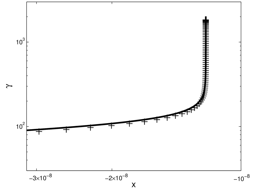
Figure 2: Lorentz factor $\gamma$ as a function of position $x$ shortly before the shock breaks out of the star. The density profile has power-law index $k=-1.5$. The analytic profile taken from the self-similar solution (solid line) agrees well with the numerical profile (crosses).

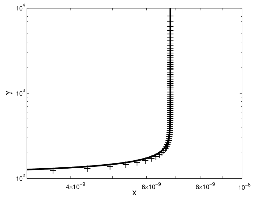
Figure 3: Same as Figure 2 but for a time shortly after the shock emerges from the star.

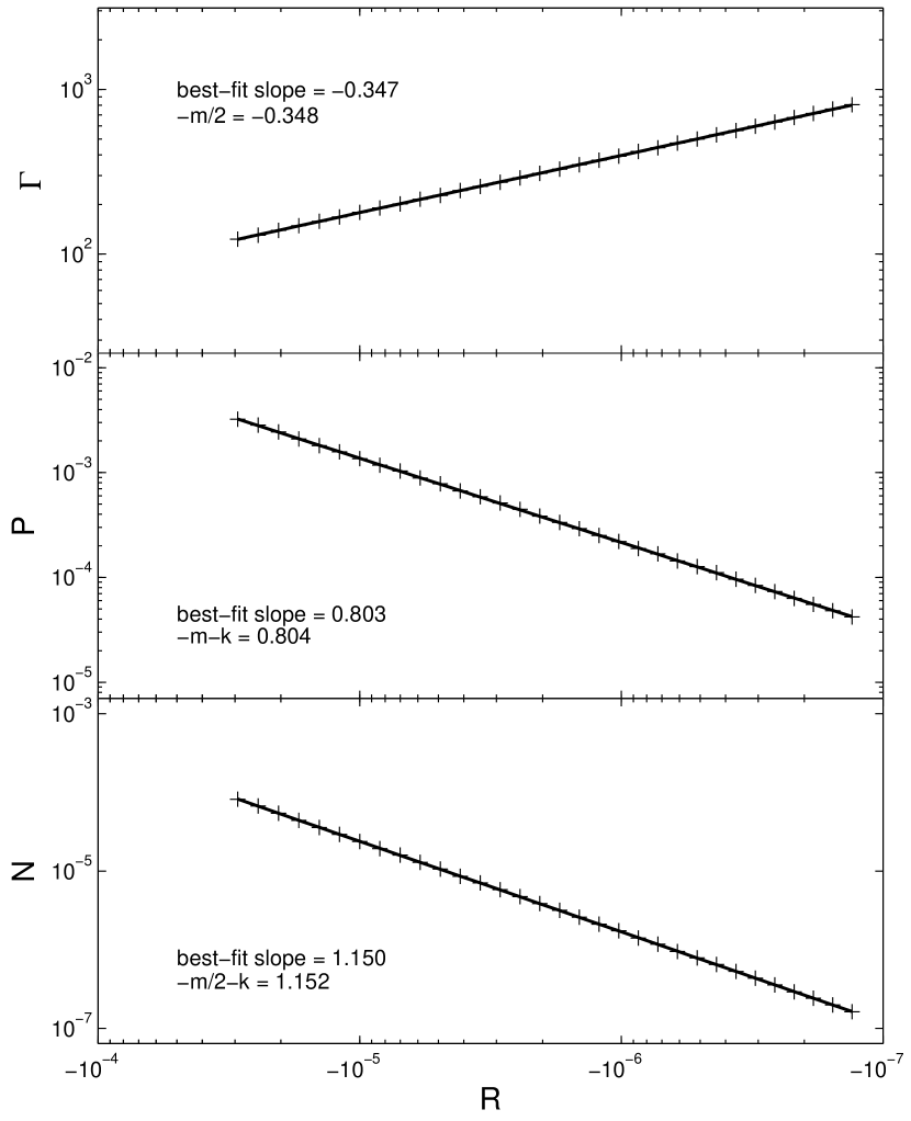
Figure 4: Evolution of $\Gamma$ (top panel), $P$ (middle panel), and $N$ (bottom panel) with $R$ while the shock is still inside the star. The density profile has power-law index $k=-1.5$. The evolution of $\Gamma$, $P$, $N$ with $R$ is equivalent to time evolution when $\Gamma\gg 1$. Crosses represent numerical data; solid lines are the best-fit lines to the data. That the data are well fit by lines implies that $\Gamma$, $P$, and $N$ do indeed evolve as power laws; that the numerical and analytic slopes agree confirms that the evolution is as expected.

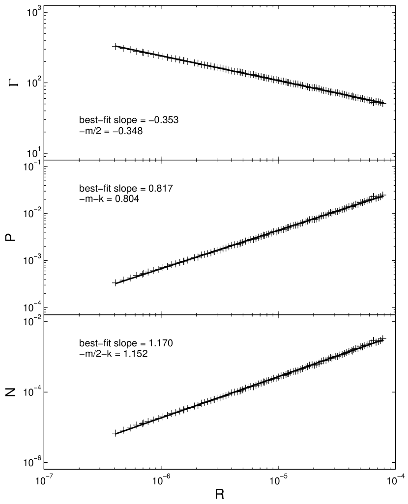
Figure 5: Same as Figure 4 but for times after the shock emerges from the star. $\Gamma$, $P$, $N$, and $R$ were deduced from the numerical data by finding at each time the position where $\gamma^{-1}p/n$, the ratio of the thermal and the bulk kinetic energies in the frame of the fluid, fell just below the constant value we expect at the time of breakout.

6 Summary

We have shown that, given an ultrarelativistic shock propagating into a planar polytropic envelope, the flow upon the shock’s emergence from the envelope into vacuum follows a self-similar solution strikingly similar to the self-similar solution describing the flow while the shock remains within the envelope. Both self-similar solutions obey the same relations with regard to the time-evolution of the characteristic quantities $R$, $\Gamma$, $P$, $N$ and with regard to the similarity variables $\chi$, $g$, $f$, $h$. The pre- and post-breakout solutions differ only in that the applicable ranges in $\chi$ and the physical interpretations of the characteristic quantities differ. As a result of these differences, the behavior of the flow after breakout lies somewhere between the traditional Type I and Type II classes of self-similar solutions; before breakout a Type II solution applies. To arrive at these results we have looked in detail at the behavior when the shock reaches the outer edge of the envelope.

We have discussed these results in the context of an application—the motion of a shock wave through a polytropic envelope near the surface of a star, the shock’s emergence from the surface, and the subsequent flow into vacuum. This situation may be related to the explosions believed to cause gamma-ray bursts and supernovae (see, for example, Tan et al., 2001) and should be especially relevant in very optically thick media such as neutron stars.

References

- Best & Sari (2000) Best, P., & Sari, R. 2000, Physics of Fluids, 12, 3029
- Blandford & McKee (1976) Blandford, R. D., & McKee, C. F. 1976, Physics of Fluids, 19, 1130
- Johnson & McKee (1971) Johnson, M. H., & McKee, C. F. 1971, Phys. Rev. D, 3, 858
- Nakayama & Shigeyama (2005) Nakayama, K., & Shigeyama, T. 2005, astro-ph 0503252
- Sari (2005) Sari, R. 2005, submitted
- Sedov (1946) Sedov, L. I. 1946, Appl. Math. Mech. Leningrad, 10, 241
- Tan et al. (2001) Tan, J. C., Matzner, C. D., & McKee, C. F. 2001, ApJ, 551, 946
- Taylor (1950) Taylor, G. I. 1950, Proc. R. Soc. London Ser. A, 201, 175
- von Neumann (1947) von Neumann, J. 1947, Blast Waves, Tech. Rep. 7, Los Alamos National Laboratories
- Waxman & Shvarts (1993) Waxman, E., & Shvarts, D. 1993, Physics of Fluids, 5, 1035
- Zel’dovich & Raizer (1967) Zel’dovich, Y. B., & Raizer, Y. P. 1967, Physics of Shock Waves and High-Temperature Phenomena (New York: Academic Press)