To see or not to see a Bow Shock:

OB–stars have the highest luminosities and strongest stellar winds of all stars, which enables them to interact strongly with their surrounding ISM, thus creating bow shocks. These offer us an ideal opportunity to learn more about the ISM. They were first detected and analysed around runaway OB–stars using the IRAS allsky survey by van Buren et al. (Buren95 (1995)). Using the geometry of such bow shocks information concerning the ISM density and its fluctuations can be gained from such infrared observations. As to help to improve the bow shock models, additional observations at other wavelengths, e.g. H$\alpha$, are most welcome. However due to their low velocity these bow shocks have a size of $\sim 1$°, and could only be observed as a whole with great difficulties. In the light of the new H$\alpha$ allsky surveys (SHASSA/VTSS) this is no problem any more.
We developed different methods to detect bow shocks, e.g. the improved determination of their symmetry axis with radial distance profiles. Using two H$\alpha$–allsky surveys (SHASSA/VTSS), we searched for bow shocks and compared the different methods. From our sample we conclude, that the correlation between the direction of both proper motion and the symmetry axis determined with radial distance profile is the most promising detection method.
We found eight bow shocks around HD 17505, HD 24430, HD 48099, HD 57061, HD 92206, HD 135240, HD 149757, and HD 158186 from 37 candidates taken from van Buren et al. (Buren95 (1995)). Additionally to the traditional determination of ISM parameters using the standoff distance of the bow shock, another approach was chosen, using the thickness of the bow–shock layer. Both methods lead to the same results, yielding densities ($\sim 1$ cm^-3) and the maximal temperatures ($\sim 10^{4}$ K), that fit well to the up–to–date picture of the Warm Ionised Medium.

1 Introduction

OB–stars are the most massive and luminous stars known with masses greater than 10 $M_{\odot}$ and effective temperatures ranging from 10 000 K up to 50 000 K. During their short lifetime ($\leq$20$\times$10⁶ yr) OB–stars lose mass at rates of $\dot{M}\approx 10^{-7}-10^{-5}\,M_{\odot}$ yr^-1 (Lamers & Cassinelli Lamers (1989)). This stellar wind with velocities of $v_{\infty}\approx 1\,000-3\,000$ km s^-1 transfers a great amount of mechanical energy to the surrounding ISM, comparable to a supernova explosion. As a result, OB–stars create a stellar bubble (Castor et al. castor (1975)) which structures the Interstellar Medium (ISM). This spherical bubble is altered when the OB–star is in motion, as wind and ISM interact directly. The resulting nebula is known as a bow–shock nebula. Recently many new bow shocks (size $\sim$1′) created by fast moving neutron stars or pulsars have been detected and analysed. Their geometry could be successfully used to gain information about the ISM, such as density and temperature (Gaensler et al. gaensler (2001)). Thus the theoretical models of such bow shocks have become quite exact recently, enabling us to glance at the missing link between density fluctuations seen in H i (at scales $\sim 0.1-200$ pc) and towards pulsars (at scales $\sim 5-100$ AU). Bow–shock nebula around OB–stars can also be used as ISM probes, if observable or rather detectable, as described in the following.
In Buren88 (1988) van Buren & McCray detected structures around OB–stars and Wolf–Rayet stars using the 60 $\mu$m allsky survey of the InfraRed Astronomical Satellite (IRAS). These images revealed an arc–like structure and a high colour temperature, possibly being bow shocks. A more complete sample of 188 runaway OB–stars was analysed by van Buren et al. (Buren95 (1995)) (hereafter VB) using the IRAS allsky survey which lead to the detection of 58 bow shocks. Because of these numerous detections and the alignment of the symmetry axis of the structures along the direction of proper motion of the central star, they could only be bow–shock nebula.
Due to the low resolution of IRAS ($\sim$1$\aas@@fstack{\prime}$5) it is difficult to determine the exact location of the bow shock and its symmetry axis. Furthermore, VB could only use the Hipparcos input catalogue (HIC) to determine the proper–motion direction of the central star. As the Hipparcos catalogue is now completed, its astrometrical data together with the almost complete H$\alpha$ allsky surveys Virginia Tech Spectral Survey¹ (VTSS; Dennison et al. dennison (1997)) and Southern Hemispheric H$\alpha$ Sky Survey Atlas (SHASSA; Gaustad et al. gaustad (2001)), the VB sample is reanalysed here, now using the H$\alpha$ emission line.
The development from a stellar bubble to a bow shock is illustrated in Sect. 2. The used H$\alpha$–data and its acquisition is described in Sect. 3. Sect. 4 explains the analysis of the bow shocks and the improved methods developed to detect them. In Sect. 5 the results of the observations are given and in Sect. 6 ISM parameters derived, followed by a discussion in Sect. 7. Finally, Sect. 8 draws a conclusion concerning the main points of this paper.

2 Scenario

For a better understanding of the methods used, the scenario of a bow shock and the source of the high velocity of the OB–stars are given.
The evolving stellar bubble, as illustrated in Fig. 1, is in its longest snowplow stage divided into four parts centred upon the OB–star (Castor et al. castor (1975)): The innermost area (A) is an unshocked and freely expanding stellar wind, followed by a larger area (B) of shocked stellar wind. These hot regions, as if they were a snowplow (hence the name of this stage), have pushed together a thinner area (C) of shocked ISM. All regions are embedded in the unshocked ISM (D).

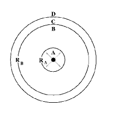
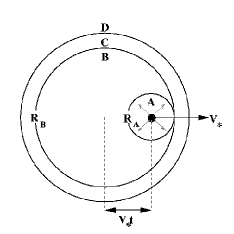
Figure 1: Structure of a stellar bubble created by a stationary star (left) and a star in motion (right). The different regions A, B, C, and D and the geometry are described in Sect. 2.

The models describing such stellar bubbles assume that the OB–star is stationary with respect to the ISM. However as all stars have a proper motion, so do OB–stars. A special population of OB–stars is known as runaway OB–stars (Blaauw Blaauw (1961)). They are defined as having a proper motion greater than 30 km s^-1. This criteria was chosen to discern them from non–runaway OB–stars, which have a velocity dispersion of about 10 km s^-1.
As runaway stars are often found in isolated regions, their high velocity cannot be explained as a motion within a stellar cluster. Two scenarios explaining observed properties of runaway OB–stars are favoured:
Firstly, the Binary–Supernova–Scenario (BSS) as described by Blaauw (Blaauw (1961)). The partner of the OB–star explodes as a Supernova (SN). Thereby the OB–star is set free with its typical orbital velocity of 30–150 km s^-1. And secondly, the Dynamical–Ejection–Scenario (DES) proposed by Hoffer (Hoffer (1983)). In this Scenario the collision of two binary systems leads to the ejection of one star with a velocity of up to 200 km s^-1.

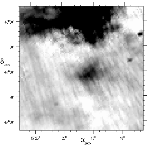
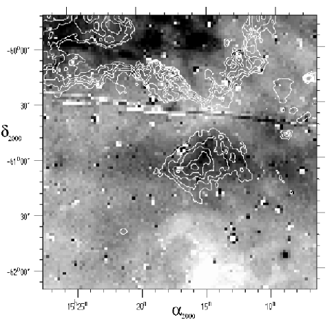
Figure 2: Left: IRAS 60 $\mu$m excess map of HD 135240. Right: Overlay of H$\alpha$ image in grey–scale and the IRAS 60 $\mu$m excess map in white contours. Both are shown with their slanted equatorial–coordinate system (J2000) and inverted grey–scale.

Taking the motion of the star ($V_{\ast}$) into account, regions A, B, and C will still be spherical as long as the stellar velocity is smaller than the sound velocity within B. However B and C are no longer centred on the star, as shown in Fig 1. If region A and D do not interact directly, this would be the only alteration to the model of the stellar bubble. But as soon as the star enters denser regions of the ISM, like molecular clouds, the cooling of region B becomes more effective. This leads to a collapse of B and C within timescales smaller than the lifetime of the OB–star, and the approach of region A and D. As molecular clouds are not frequently encountered, region A and D can only interact when the offset of A to B and C is $V_{\ast}t\approx R_{B}(t)-R_{A}(t)$. Where the timescale is dependent upon the velocity of the OB–star and the density of the surrounding ISM. Taking typical values of the lifetime and velocity $V_{\ast}$=39 km s^-1 this leads to a density constraint of $n\geq 0.017$ cm^-3 in which A and D can interact directly.
In the case of directly interacting unshocked stellar wind and unshocked ISM, the geometry is changed completely. As Wilkin (Wilkin (1996)) describes, the ram pressure of both media can be balanced directly and result in a bow shock. This bow shock is axi–symmetric along the direction of proper motion and can be approximated by a parabola. The two layers B and C of the model above are mixed due to turbulence and plasma instabilities leading to a single layer in which the material of the ISM and stellar wind moves along the bow shock. The material in this has experienced a nearly isothermal shock, so its density is higher than that of the surrounding ISM. This leads to the creation of warm interstellar dust best seen in 60 $\mu$m, and the OB–star in the centre leads to the ionisation of the layer emitting H$\alpha$.

3 Data

3.1 Selection

The data used for this program were taken from the SHASSA and incomplete VTSS allsky surveys. SHASSA contains the southern hemisphere up to $\delta$=15° and VTSS the northern hemisphere down to $\delta=$–15°. Both surveys were made with a CCD detector and a fast photo–objective of $\sim$55 mm at $\sim$f/1.4, leading to a field of view of $\sim$13°. All images were integrated $\sim$25 min resulting in a detection limit down to $\sim$0.75 rayleigh $\left(1\,{\rm R}=\frac{10^{6}}{2\pi}\frac{\rm Photons}{\rm cm^{2}\,\rm s\,\rm sr}\right)$. Due to the different pixel sizes of the detectors SHASSA has a resolution of 0$\aas@@fstack{\prime}$8 and VTSS of 1$\aas@@fstack{\prime}$6.
The H$\alpha$–sample used consists of the O–stars taken from the VB sample with data from either VTSS or SHASSA, ensuring a sufficient Lyman continuum flux to ionise the bow–shock layer.
We searched for bow shocks around these 37 candidates of the H$\alpha$–sample within the SHASSA and VTSS H$\alpha$ survey. Due to always present background nebulosity, it had to be ensured that the structures seen were really bow shocks. As described at the end of Sect. 2, the bow–shock layer should be visible in 60 $\mu$m as well as in the H$\alpha$ emission line. Therefore, the H$\alpha$ images were compared with the 60 $\mu$m IRAS images of the same region. Though the IRAS images show a great amount of nebulous emission, the nebulosity can successfully be subtracted using the 100 $\mu$m images of IRAS. This correction has been done based on the recipe of VB with the creation of IRAS 60 $\mu$m excess maps, shown for the example of HD 135240 in Fig. 2.
To compare both images with each other, the contours of the IRAS 60 $\mu$m excess map were overlaid upon the H$\alpha$ images (see Fig. 2). We used this image to decide whether a bow shock seen in the IRAS 60 $\mu$m excess map is also present within the H$\alpha$ image. The eight bow shock detections and a short description of the comparison using the overlays are given in Table 1. The IRAS 60 $\mu$m excess images and their corresponding H$\alpha$ images are also shown in Fig. 8 and Fig. 9.

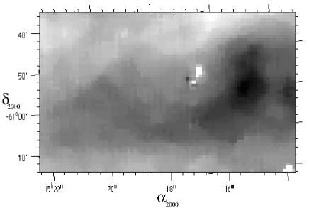
Figure 3: Median filtered section of the H$\alpha$ image containing the bow shock around HD 135240. The coordinate system and grey–scale as in Fig. 2.

To check for the positioning quality of the H$\alpha$ image compared to the IRAS 60 $\mu$m excess maps in the overlays, we could not use the nebulosities as criteria. As we are using these overlays to see coinciding positions of nebulosities within both images this would be misleading. Better criteria are point sources like stars which have to be visible with IRAS and in VTSS/SHASSA, thus, we used the positions of M giants as a reference. Using this method, a deviation of the positional offsets of $\sigma=20$″ was measured, which is sufficiently smaller than the resolution of both images.
To analyse the H$\alpha$ images of the selected bow shocks only the interesting region was extracted. As only the search for bow shocks using the overlays requires the best possible resolution of 1.6′ (VTSS) and 0.8′ (SHASSA), the images could for further analysis be median filtered with a $5\times 5$ pixel wide box (see Fig. 3 for the example of HD 135240). The resulting improvement of S/N leads to a decreased resolution of 8′ (VTSS) and 4′ (SHASSA).

Table 1: Surveys containing the candidates of the H$\alpha$–sample; bow–shock detections as results from the overlay are printed in bold letters.

$$\begin{array}[]{p{0.2\linewidth}p{0.25\linewidth}p{0.4\linewidth}}\hline\cr\vskip 3.0pt plus 1.0pt minus 1.0pt\cr Star&Survey&Bow Shock\\ \vskip 3.0pt plus 1.0pt minus 1.0pt\cr\hline\cr\vskip 3.0pt plus 1.0pt minus 1.0pt\cr HD 1337&VTSS&ambiguous\\ \bf HD 17505&\bf VTSS&\bf complicated background\\ HD 19820&VTSS&weak\\ \bf HD 24431&\bf VTSS&\bf detection\\ HD 30614&{\sl(VTSS)}&{\sl not in survey}\\ HD 34078&{\sl(VTSS)}&{\sl not in survey}\\ BD +39 1328&VTSS&non--detection\\ HD 37020&VTSS/SHASSA&ambiguous\\ HD 41161&{\sl(VTSS)}&{\sl not in survey}\\ HD 41997&VTSS&ambiguous\\ HD 47839&VTSS&non--detection\\ \bf HD 48099&\bf VTSS/SHASSA&\bf complicated background\\ HD 52533&SHASSA&non--detection\\ HD 54662&VTSS/SHASSA&ambiguous\\ \bf HD 57061&\bf SHASSA&\bf detection\\ HD 64315&SHASSA&ambiguous\\ HD 66811&SHASSA&non--detection\\ \bf HD 92206&\bf SHASSA&\bf small\\ HD 101131&SHASSA&non--detection\\ HD 112244&SHASSA&non--detection\\ HD 130298&SHASSA&ambiguous\\ \bf HD 135240&\bf SHASSA&\bf detection\\ HD 329905&SHASSA&non--detection\\ \bf HD 149757&\bf SHASSA&\bf detection\\ HD 156212&SHASSA&ambiguous\\ \bf HD 158186&\bf SHASSA&\bf complicated background\\ HD 164492&SHASSA&non--detection\\ HD 169582&SHASSA&ambiguous\\ HD 175514&VTSS&weak\\ HD 186980&{\sl(VTSS)}&{\sl not in survey}\\ HD 188001&VTSS&non--detection\\ HD 227018&{\sl(VTSS)}&{\sl not in survey}\\ HD 195592&{\sl(VTSS)}&{\sl not in survey}\\ HD 199579&VTSS&incomplete scan\\ HD 203064&VTSS&non--detection\\ HD 210839&{\sl(VTSS)}&{\sl not in survey}\\ HD 214680&VTSS&non--detection\\ \vskip 3.0pt plus 1.0pt minus 1.0pt\cr\hline\cr\end{array}$$

3.2 Distances

To convert angular sizes into linear sizes, the distances of the eight bow–shock candidates had to be determined. Additionally, the interstellar absorption had to be calculated to fit the brightness profile correctly.
Due to the high parallax errors determined by Hipparcos for the candidates the distances were determined using their spectral parallax with absolute magnitudes derived from Landolt–Börnstein (Landolt (1982)) according to the spectral classification described in appendix A. As for the absorption along the line of sight, photometric data for the B and V filters were taken, and the normal extinction law (Mathis, Mathis (1990)) applied. The expected absorption within the H$\alpha$–line was estimated according to the interstellar extinction given by Mathis (Mathis (1990)).
In appendix A the magnitudes and multiplicity of the different sources are described. All data and results are given in Table 2.

Table 2: Photometry and astrometry of the central stars of the bow–shock candidates. $m_{B}$ and $m_{V}$ are the apparent B and V magnitudes, $\mu_{\alpha}$ and $\mu_{\delta}$ give the proper motion along the rightascension and declination axis, and $V_{r}$ is the radial velocity. The spatial velocity $V$, the symmetry axis position $\theta_{a}$ and its inclination $\iota_{\mathrm{A}}$ are derived from the astrometric data. The distance $r$ is derived from the spectral parallax.

$$\begin{array}[]{p{0.1\linewidth}p{0.08\linewidth}p{0.1\linewidth}llr@{\pm}l r@{\pm}l r@{\pm}l l r@{\pm}l r@{\pm}l l}\hline\cr\vskip 3.0pt plus 1.0pt minus 1.0pt\cr star&SC&multiplicity&m_{B}&m_{V}&\lx@intercol\hfil\mu_{\alpha}\hfil\lx@intercol&\lx@intercol\hfil\mu_{\delta}\hfil\lx@intercol&\lx@intercol\hfil V_{r}\hfil\lx@intercol&V&\lx@intercol\hfil r\hfil\lx@intercol&\lx@intercol\hfil\theta_{a}\hfil\lx@intercol&\iota_{\mathrm{A}}\\ &&&[{\rm mag}]&[{\rm mag}]&\lx@intercol\hfil[{\rm mas\,yr}^{-1}]\hfil\lx@intercol&\lx@intercol\hfil[{\rm mas\,yr}^{-1}]\hfil\lx@intercol&\lx@intercol\hfil{\rm km\,s}^{-1}\hfil\lx@intercol&{\rm km\,s}^{-1}&\lx@intercol\hfil[{\rm pc}]\hfil\lx@intercol&\lx@intercol\hfil[\degr]\hfil\lx@intercol&[\degr]\\ \vskip 3.0pt plus 1.0pt minus 1.0pt\cr\hline\cr\vskip 3.0pt plus 1.0pt minus 1.0pt\cr HD 24431&O9 IV--V&binary&7.2&6.9&-0.21&1.01&-1.52&0.86&-9.9&2&12.0&911&57&262&38&56\\ HD 48099&O7 V&binary&6.3&6.4&+0.81&0.65&+2.35&0.53&+31&2&37.7&1829&77&71&15&55\\ HD 57061&O9 II&quintuple&6.0&6.1&-1.82&0.44&+3.74&0.59&+40.4&2&55.8&1914&79&116.0&6.5&46\\ HD 92206&O6 ?&binary&8.3&8.2&-10.4&4.2&+6.8&4.2&-10&5&40.5&4049&109&147&19&1\\ HD 135240&O7 III-V&triple&5.0&5.1&-2.02&0.51&-4.08&0.55&+9.2&2&32.5&1131&63&243.7&6.5&16\\ HD 149757&O9 V&single&2.6&2.6&+13.07&0.86&+25.44&0.71&-15&10&26.8&163&27&62.8&1.6&34\\ HD 158186&O9.5 V&binary&7.0&7.0&+1.36&1.11&-1.26&0.48&\lx@intercol\hfil-9\hfil\lx@intercol&13.9&1094&62&317&26&41\\ HD 17505&O6.5 V&binary?&7.8&7.4&-1.38&1.16&-0.69&1.08&-17&5&25.7&1416&69&207&41&41\\ \vskip 3.0pt plus 1.0pt minus 1.0pt\cr\hline\cr\end{array}$$

3.3 Motion

The proper motion of the eight bow–shock candidates was taken from the Hipparcos–catalogue, as well as their errors derived from the given error–ellipse. The radial velocity information was taken from CDS (Evans D. S. evans (1979); Wilson R. E. wilson (1953)). Only in the case of HD 158186 was this value updated with respect to the ones given in VB. The astrometric data led to the determination of the inclination and the position angle of the proper motion concerning the central stars of the bow–shock candidates. The astrometric results are given in Table 2 .
If the nebula were created by a bow shock, these parameters should be the same as for the bow shocks. The inclination can be directly compared. As for possible image rotation of the H$\alpha$ image compared to the global coordinate system, neighbouring stars were measured and the position angle corrected.

4 Analysis

Bow–shock nebulae are structures which appear limb brightened, due to their shell like geometry. Assuming that the gas within the layer is optically thin, one can compute qualitatively the characteristics of a brightness profile by determining the length of the line of sight within the layer. When plotting this profile against the radial distance of the line of sight, one obtains radial brightness plots as shown in Fig. 4. Case A demonstrates the situation of limb darkening for a sphere, while B shows the radial brightness plot of a spherical shell. The radial brightness plot of a bow shock is that of case C. The inner boundary of the layer was described by a parabola, as van Buren et al. (Buren90 (1990)) suggested. The outer boundary was described by a confocal parabola ensuring a constant thickness of the layer. The similar appearance of radial brightness plot B and C will be discussed later.

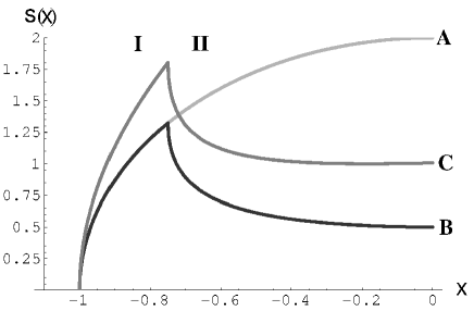
Figure 4: Theoretical radial brightness plot for a sphere (A) light grey, a spherical shell (B) dark grey and a bow–shock layer (C) medium grey. They are derived from the line of sight $s(x)$ through the regions, with the star at the position $x=0$. I and II are the exterior and interior of the different regions.

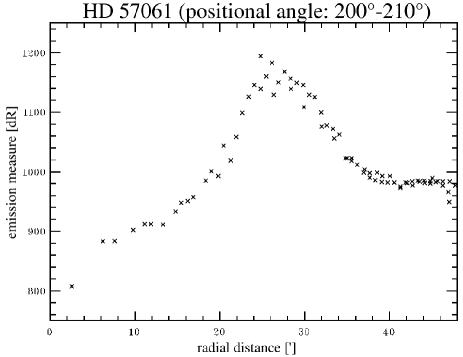
Figure 5: The measured radial brightness plot of HD 57061 with the radial distance from the central O–star.

For all eight candidates, detected using IRAS 60 $\mu$m excess maps (see Sect. 3.1), radial brightness plots were derived by transforming the pixel coordinates of the images into a polar coordinate system centred upon the central O–star. The surface H$\alpha$ brightness of all pixels within a 10° wide wedge were then plotted against their radial distance in arcmin. A resulting radial brightness plot for HD 57061 is shown in Fig. 5, demonstrating the typical limb brightening of a bow shock superimposed upon a nearly constant background emission.
The measurement of the symmetry axis of the bow–shock nebula was verified with a method, other than that proposed by VB. When applying their method one determines the symmetry axis of the structure created by the bow shock and the background emission together. This would alter the direction of the bow–shocks symmetry axis. If one could determine the location of the inner boundary of the bow–shock layer free of background contaminations, it would be possible to determine the symmetry axis of the bow shock by itself. This can be achieved using the location of the maximum of the radial brightness plot. The maximum is determined by the varying brightness of the bow shock alone. Background nebulosity will most certainly not be so sharply peaked. Therefore, its location exactly traces the inner boundary.
The radial distance of the inner boundary was traced with radial brightness plots for each bow–shock candidate. Plotting the distance against the position angle of the wedge used to create the radial brightness plot, results in a radial distance profile as shown on the right of Fig. 6 for the example of HD 158186. The radial distance profile shows a symmetric behaviour and its symmetry axis coincides with that of the bow–shock structure. Taking the existence of a symmetry axis for granted the position of the axis is determined by a symmetric function fitted to the data points, which also coincides with the symmetry axis of the bow shock. A parabola:

$$r=a(\theta-\theta_{s})^{2}+b$$ (1)

was chosen to fit the data because of its few free parameters and its close approximation of the data. The parabola is fitted to the data plotted in polar coordinates. A parabola in cartesian coordinates, for which the parabola of van Buren et al. (Buren90 (1990)) in Eq. 2 is defined, can be transformed, but would be of a more complicated structure not needed to measure the symmetry axis. Resulting from the great width of the wedge, only few radial brightness plots were created, thus only few data points were present in the radial distance profiles, but enough to ensure a symmetric distribution (see open or filled circles on the right of Fig. 6). To double the data points and gain a more precise symmetry axis position the points were mirrored with an assumed symmetry axis $\theta_{s}$. Thereafter, the parabola (Eq. 1) was fitted to the points, using the least–square method and error weighting (as for all following fits), keeping the displacement $\theta_{s}$ constant. In steps of 0$\aas@@fstack{\circ}$1, $\theta_{s}$ was changed and an variance $s^{2}$ of the fit derived. The symmetry axis was chosen to be at a $\theta_{s}$ of minimal variance (see the left of Fig. 6 for the example of HD 158186), which agrees with the less precise value found without mirroring. The errors of $\theta_{s}$ result from a final fit allowing for $\theta_{s}$ to vary. All symmetry axes are given in Table 3.
The comparison of all position angles determined either by VB or through radial distance profile or astrometry are given in Table 4, also noting the deviation of radial distance profile with respect to the astrometric results.

Table 3: Derived parameters of the analysed bow shocks. $\theta_{\rm s}$ and $\iota$ are the position and inclination of the symmetry axis using the H$\alpha$ images. The standoff distances SOD are given for the two cases of no inclination and inclination. d is the thickness of the bow–shock layer perpendicular to its surface. Uncertain values are given without errors.

$$\begin{array}[]{p{0.18\linewidth}r@{\pm}lr@{\pm}lr@{\pm}lr@{\pm}lr@{\pm}l}\hline\cr\vskip 3.0pt plus 1.0pt minus 1.0pt\cr star&\lx@intercol\hfil\theta_{\rm s}\hfil\lx@intercol&\lx@intercol\hfil SOD(\iota=0\degr)\hfil\lx@intercol&\lx@intercol\hfil SOD(\iota)\hfil\lx@intercol&\lx@intercol\hfil\iota\hfil\lx@intercol&\lx@intercol\hfil d\hfil\lx@intercol\\ &\lx@intercol\hfil[\degr]\hfil\lx@intercol&\lx@intercol\hfil[\arcmin]\hfil\lx@intercol&\lx@intercol\hfil[\arcmin]\hfil\lx@intercol&\lx@intercol\hfil[\degr]\hfil\lx@intercol&\lx@intercol\hfil[10^{15}\,{\rm cm}]\hfil\lx@intercol\\ \vskip 3.0pt plus 1.0pt minus 1.0pt\cr\hline\cr\vskip 3.0pt plus 1.0pt minus 1.0pt\cr HD 57061&202.8&2.0&13.56&0.16&6&11&75&40&16.9&4.4\\ HD 92206&79.9&4.1&3.11&0.16&3.9&1.8&0&10&9.8&2.7^{1}\\ HD 158186&238.3&1.7&5.96&0.13&7.4&1.4&\lx@intercol\hfil 0\hfil\lx@intercol&1.80&0.11\\ HD 135240&296.7&1.7&10.65&0.16&13.3&1.6&\lx@intercol\hfil 0\hfil\lx@intercol&2.90&0.42\\ HD 149757&67.1&1.7&9.42&0.18&0&48&\lx@intercol\hfil 90\hfil\lx@intercol&\lx@intercol\hfil\cdots\hfil\lx@intercol\\ HD 17505&358.1&3.8&5.82&0.18&5.8&2.1&\lx@intercol\hfil 0\hfil\lx@intercol&0.59&0.07\\ HD 24431&312&3.1&7.10&0.32&5.6&13&71&49&6.6&1.0\\ HD 48099&238.6&5.3&4.25&0.25&\lx@intercol\hfil 0\hfil\lx@intercol&90&0.8&2.25&0.62\\ \vskip 3.0pt plus 1.0pt minus 1.0pt\cr\hline\cr\end{array}$$

• Layer thickness of HD 92206 is given in $10^{9}$ cm

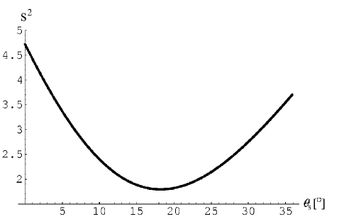
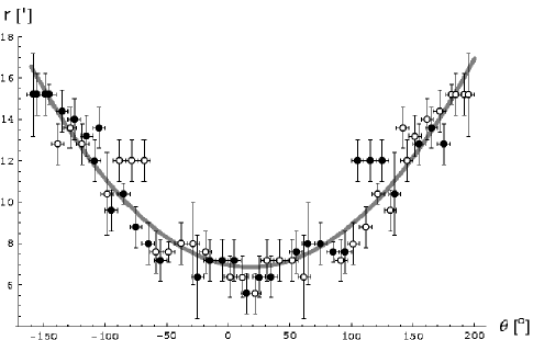
Figure 6: Left: The variance $s^{2}$ of different symmetry axis $\theta_{\rm s}$ referring to an arbitrary axis for HD 158186. Right: The radial distance profile of HD 158186 with the position angle $\theta$ as used in the left figure. Symmetry axis is chosen as the minimum of $s^{2}$. Open circles indicate the mirrored data.

The data is transformed back to a cartesian coordinate system with the x–axis as symmetry axis. Now, the physically motivated parabola of van Buren et al. (Buren90 (1990))

$$z=\frac{y^{2}}{3R_{0}}-R_{0}$$ (2)

can be fitted to the data of $\theta=[-90\degr,+90\degr]$ nearest the apex. The parameter $R_{0}$ so determined is known as the standoff distance, and is used to calculate ISM densities. Eq. 2 is only correct for an inclination of $\iota=0$ and thus, $R_{0}$ represents an upper limit. The rotated parabola $\left(z(x,y)=\frac{x^{2}+y^{2}}{3R_{0}}-R_{0}\right)$ with a different inclination angle $\iota$ is more complex:

$$z(y)=\frac{y^{2}}{3R_{0}}\cos\iota-R_{0}\left(\frac{3R_{0}}{4}\tan^{2}\iota+1\right)\cos\iota\quad.$$ (3)

Both parabolas were fitted to the data of all eight bow–shock candidates. The standoff distance with or without inclination and the inclination $\iota$ are given in Table 3 .
A further important parameter characterising a bow shock is the thickness $d$ of the bow–shock layer. To determine $d$, one plots the variation of the brightness of the inner boundary, derived from the radial brightness plots, against the position angle relative to the symmetry axis resulting in a brightness profile, shown for HD 57601 in Fig. 7. The brightness is given as an emission measure which can be approximated as $EM=n_{s}^{2}s$ in case of a homogeneous density $n_{s}$ within the bow–shock layer and the length of the line of sight $s$ through the layer. Near the apex of the parabola and at an inclination of $\iota=0\degr$, a segment of the layer can be approximated by a spherical shell of thickness $d$. In the case of photoionisation equilibrium,

$$\frac{Q}{4\pi}=r^{2}\alpha_{H\alpha\,A}(T)n_{s}^{2}d=r^{2}\alpha_{H\alpha\,A}(T)EM_{\perp}(d,r)$$ (4)

is valid. Q is the Lyman continuum flux of the O–star as given for a specific spectral type by Panagia (Panagia (1973)) and $\alpha_{H\alpha\,A}=5.83\times 10^{-14}$ cm³ s^-1 is the recombination coefficient for the H$\alpha$ line at $T=10\,000$ K derived from Osterbrock (Osterbrock (1989)). Here, the emission measure $EM_{\perp}$ is only valid when looking directly through the bow–shock layer. The maximum EM we measure is given as $EM(d,r)=2EM_{\perp}(d,r)\sqrt{2\frac{r}{d}+1}$. For the parabola of Eq. 2 the radial distance can be calculated as:

$$r(x)=\sqrt{x^{2}+\left(\frac{x^{2}}{3R_{0}}-R_{0}\right)^{2}}$$ (5)

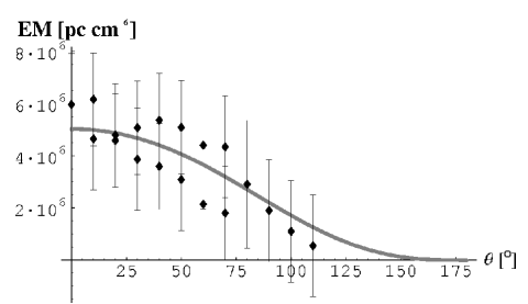
Figure 7: The brightness profile of HD 57061 resulting in a thickness $d=(16.9\pm 4.4)\times 10^{15}$ cm.

and the polar angle $\theta=\arctan\frac{x}{z}+90\degr$ is given by:

$$x(\theta)=\frac{3}{2}a\tan\theta\pm\sqrt{\frac{3}{2}a^{2}\tan^{2}\theta+3a^{2}}\quad.$$ (6)

This together leads to a brightness profile of:

$$EM(d,\theta)=\frac{Q\sqrt{\frac{2r(\theta)}{d}+1}}{2\alpha_{H\alpha\,A}\pi r^{2}(\theta)}$$ (7)

that has to be fitted to the points of the brightness profile, after one has subtracted a typical value of the emission measure of the background measured at the edge of the images. In addition, an absorption correction has to be applied as well as a transformation of angular to linear distances using the distances of the O–stars, both calculated in Sect. 5. The function of Eq. 7 was fitted and the results are given in Table 3 . In the case of HD 149757, the determination of $d$ was impossible due to the saturation of the O–star contaminating the edge of the bow shock (see Fig. 8).

Table 4: The symmetry axis determined with the IRAS 60 $\mu$m excess maps ($\theta_{\rm p}$), H$\alpha$–images ($\theta_{\rm s}$), and derived from the astrometric data ($\theta_{\rm a}$) are given and compared using the deviation $\Delta\theta=\theta_{\rm a}-\theta_{\rm s}$. All angles are given in deg.

$$\begin{array}[]{p{0.2\linewidth} l r@{\pm}l r@{\pm}l r@{\pm}l}\hline\cr\vskip 3.0pt plus 1.0pt minus 1.0pt\cr star&\theta_{p}&\lx@intercol\hfil\theta_{\mathrm{s}}\hfil\lx@intercol&\lx@intercol\hfil\theta_{\mathrm{a}}\hfil\lx@intercol&\lx@intercol\hfil\Delta\theta\hfil\lx@intercol\\ \vskip 3.0pt plus 1.0pt minus 1.0pt\cr\hline\cr\vskip 3.0pt plus 1.0pt minus 1.0pt\cr HD 24431&160&226.0&3.1&262&38&36&41\\ HD 48099&340&301.4&5.3&71&15&230&20\\ HD 57061&\cdots&348.2&2.0&116.0&6.5&232.2&8.5\\ HD 92206&166&112.1&4.1&147&19&35&23\\ HD 135240&145&250.3&1.7&243.7&6.5&6.3&8.2\\ HD 149757&290&115.9&1.7&62.8&1.6&52.9&3.3\\ HD 158186&\cdots&306.7&1.7&317&26&10&28\\ HD 17505&154&183.9&3.8&207&41&23&45\\ \vskip 3.0pt plus 1.0pt minus 1.0pt\cr\hline\cr\end{array}$$

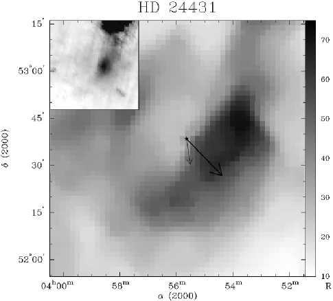
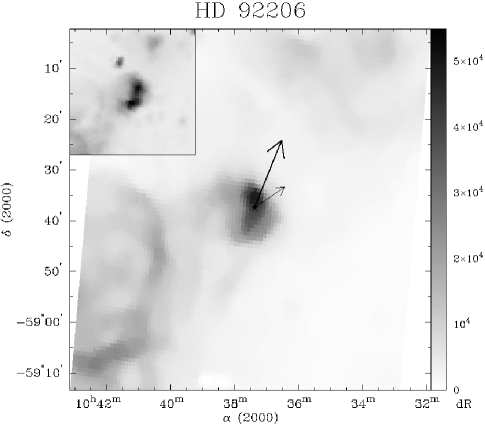
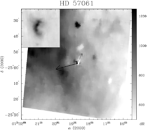
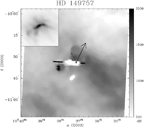
Figure 8: Median filtered H$\alpha$ images of the first four bow–shock candidates. The short arrow indicates the proper motion direction of the star and the long arrow the position of the symmetry axis. The position of the star is given by a star symbol. The grey–scales used are given in rayleigh (R) or decirayleigh (dR). The inset shows the IRAS 60 $\mu$m excess images of the bow–shock candidates used to determine the overlays, their size scaled to the H$\alpha$ images and using inverted grey–scales.

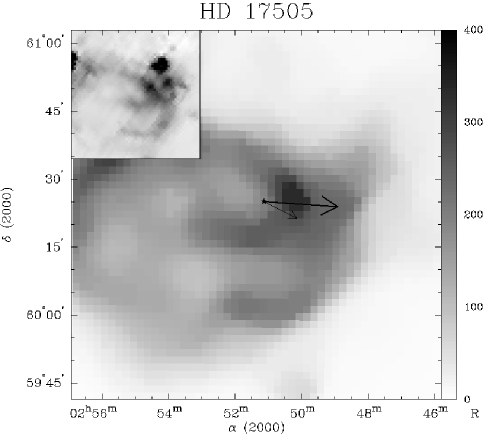
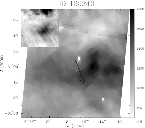
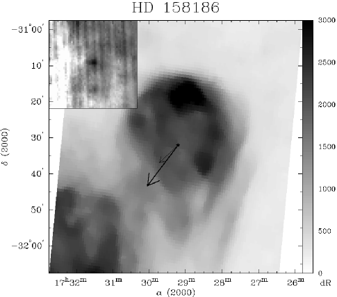
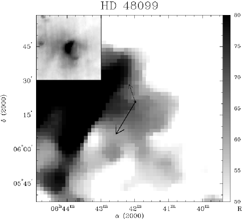
Figure 9: Median filtered H$\alpha$ images of the last four bow–shock candidates with their IRAS 60 $\mu$m excess images, symbols are defined as in Fig. 8.

5 Results

It can be seen in Eq. 2, that the standoff distance $R_{0}$ is the main parameter determining the structure of a bow shock. The distance of the bow–shock layer at the apex of the parabola, which is the standoff distance, is determined in the frame of reference of the central star by the balance of the ram pressure of the stellar wind and that of the moving ISM. The exact formula of $R_{0}$ is given by Wilkin (Wilkin (1996))

$$R_{0}=\sqrt{\frac{\dot{M}_{w}V_{w}}{4\pi n_{SOD,0}V^{2}_{\ast}}}\quad.$$ (8)

To further derive the density of the surrounding ISM $n_{SOD,0}$, the mass loss rate $\dot{M}_{w}$ and the asymptotic velocity $V_{w}$ were taken from the literature (see footnotes in Table 5). If non were present, the relations of van Buren (Buren83 (1983)) and van Buren (Buren85 (1985)) based on the luminosity and effective temperature as given by Panagia (Panagia (1973)) for the appropriate spectral class were used to calculate the missing parameters.
Due to the large errors of the standoff distance when taking the inclination into account, only uninclined standoff distances were used to derive the ISM density. Therefore, all derived ISM densities summarised in Table 5 are lower limits.
The temperature of the surrounding ISM is derived due to the fact that a bow shock can only be created when the central star has supersonic velocity $\left(M=\frac{V_{\ast}}{C_{s}}\geq 1\right)$ with respect to the surrounding ISM. The local sound velocity within a neutral medium is

$$C_{s}=\sqrt{\frac{\gamma kT}{\mu n_{SOD,0}}}\quad,$$ (9)

whereby $k$ is the Boltzmann–coefficient and the adiabatic exponent is assumed as $\gamma=\frac{5}{3}$, because the mean mass per particle and proton mass is $\mu=0.61$, when the Helium fraction is 0.1. As any velocity higher than sound speed can create a bow shock, the derived temperature is only a maximal one and also given in Table 5.
As one has derived the thickness $d$, measured the maximum EM of the bow–shock layer, and therefore $EM_{\perp}$, the density of the layer can be derived using the definition of the EM$=n_{s}d$. The surface density at the apex (cf. Wilkin, Wilkin (1996))

$$\sigma=n_{s}d=\frac{3}{4}R_{0}n_{LT,0}\left(1+\frac{V_{\ast}}{V_{w}}\right)^{2}$$ (10)

then leads to an alternative calculation of the ISM density $n_{LT,0}$ (Table 5).

6 Discussion

The results are discussed in three parts. First, the individual characteristics of the different candidates are mentioned and the problems encountered while analysing them. Second, the quality of the developed methods to detect bow shocks and determine their parameters are discussed. And thirdly, the sample and its characteristics as a whole are described and elucidated.

Table 5: The ISM parameters $n_{SOD,0}$ and $T_{max}$ as derived from the standoff distance ($R_{0}$), compared to $n_{LT,0}$ as derived from bow–shock layer density ($n_{s}$), using mass loss rates and stellar wind velocities taken from the literature as cited in the footnotes.

$$\begin{array}[]{p{0.2\linewidth} r@{\pm}l r@{\pm}l l r@{\pm}l r@{\pm}l}\hline\cr\vskip 3.0pt plus 1.0pt minus 1.0pt\cr star&\lx@intercol\hfil R_{0}\hfil\lx@intercol&\lx@intercol\hfil n_{SOD,0}\hfil\lx@intercol&T_{max}&\lx@intercol\hfil n_{s}\hfil\lx@intercol&\lx@intercol\hfil n_{LT,0}\hfil\lx@intercol\\ &\lx@intercol\hfil[{\rm pc}]\hfil\lx@intercol&\lx@intercol\hfil[{\rm cm}^{-3}]\hfil\lx@intercol&[10^{3}\,{\rm K}]&\lx@intercol\hfil[10^{3}\,{\rm cm}^{-3}]\hfil\lx@intercol&\lx@intercol\hfil[{\rm cm}^{-3}]\hfil\lx@intercol\\ \vskip 3.0pt plus 1.0pt minus 1.0pt\cr\hline\cr\vskip 3.0pt plus 1.0pt minus 1.0pt\cr HD 24431${}^{\mathrm{ad}}$&1.89&0.05&3.3&0.2&6.37&3.91&0.34&2.93&0.70\\ HD 48099${}^{\mathrm{bd}}$&2.26&0.10&0.18&0.02&62.9&4.8&2.1&1.5&1.0\\ HD 57061${}^{\mathrm{cd}}$&7.56&0.13&0.07&0.002&138&4.28&0.76&12.4&5.4\\ HD 92206${}^{\mathrm{aa}}$&3.67&0.19&0.007&0.001&7260&4810&340&5.2&1.8^{1}\\ HD 135240${}^{\mathrm{bd}}$&3.50&0.08&0.21&0.01&46.8&4.56&0.95&1.43&0.50\\ HD 149757${}^{\mathrm{bd}}$&0.45&0.02&1.5&0.1&31.8&\lx@intercol\hfil\cdots\hfil\lx@intercol&\lx@intercol\hfil\cdots\hfil\lx@intercol\\ HD 158186${}^{\mathrm{aa}}$&1.90&0.05&2.0&0.1&8.55&7.3&3.2&2.96&1.5\\ HD 17505${}^{\mathrm{bd}}$&1.20&0.04&21&1&29.2&23.6&1.9&2.47&0.50\\ \vskip 3.0pt plus 1.0pt minus 1.0pt\cr\hline\cr\end{array}$$

• ISM density of HD 92206 is given in $10^{-3}$ cm^-3

• van Buren (Buren83 (1983)) and van Buren (Buren85 (1985))

• Howarth & Prinja (howarth89 (1989))

• Lamers & Leitherer (lamers (1993))

• Howarth et al. (howarth97 (1997))

6.1 Candidates

As can be seen in Fig. 9 and Table 4 the symmetry axis of the bow–shock candidate around HD 48099 deviates greatly from the proper motion direction. Due to the neighbouring ISM cloud which dominates the bow–shock nebula in the northeastern side, the axis is located along the main axis of the neighbouring ISM cloud.
In case of HD 149757 the saturation of the central star causes ’bleeding’ through the bow–shock nebula (see Fig. 8) and leads to an erroneous direction of the symmetry axis (see Table 4). As before the deviation is in the expected direction, opposite to the defective region.
For HD 57061 no explanation can be found for the deviation of the symmetry axis. The nebula shows typical properties of a bow–shock nebula like its limb brightening (Fig. 5), as well as the double hump feature at the apex, seen in Fig. 8, predicted by Mac Low et al. (MacLow (1991)) for bow shocks inclined like HD 57061. This could be a hint to a possible misdirection of the astrometrically determined proper–motion direction of HD 57061.
The bow shock around HD 92206 could not be resolved completely. Therefore the derived ISM parameters deviate from the expected values for the Warm Ionised Medium (WIM).
Comparing the symmetry axis $\theta_{s}$ from the H$\alpha$ images with those derived from the astrometric data $\theta_{a}$ in Table 4 it can be said, that they coincide within their errors. Only the above mentioned cases show a significant misalignment. The same can be said, when comparing the ISM parameters with expected values for the WIM. All in all the case of the eight candidates being bow shocks can be significantly strengthened.
As for the spatial velocity noted in Table 2, the following can be said: the large errors of the velocities of HD 149757 and HD17505 are sufficient to classify them as runaways. As for HD 149757, it is a long known runaway star (cf. Hoogerwerfer et al. Hoogerwerfer (2001)). The determined spacial velocities of HD 24431 and HD 158186 are much lower than the runaway limit, thus the runaway character is uncertain. However the nebulae detected are most certainly bow–shock nebulae. The remaining four candidates have typical velocities for a runaway OB–star. The radial brightness plot derived using the H$\alpha$ images only shows the expected profile of a bow shock in case of a few position angles. All profiles only show the brightening of the nebula toward its limb, due to the strong background emission. These profiles are sufficient to determine the position of the inner boundary of the bow–shock nebula, but are useless as a sole indicator for a bow shock.

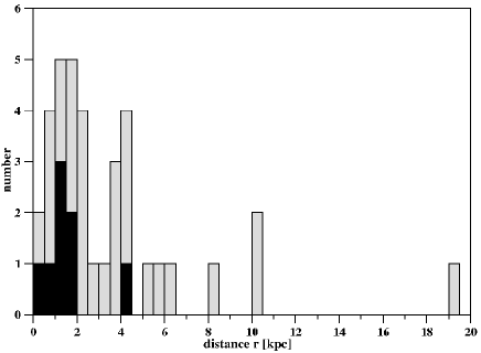
Figure 10: The stellar distance histogram of the complete H$\alpha$ sample. The bow–shock detections are plotted in black.

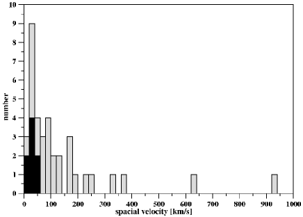
Figure 11: The stellar space velocity histogram of the complete H$\alpha$ sample, as in Fig. 10.

The best indicator is the correlation of proper–motion and symmetry–axis direction. Deriving radial distance profiles and their symmetry–axis have been shown to be robust against bright background emission, through the use of radial brightness plot, as mentioned above. The deviations from the expected profile can easily be analysed and put into context with the surrounding ISM, for example when encountering an ISM gradient.
Comparing ISM parameters derived from the bow–shock structure with expected WIM parameters is also a promising method of clarifying the bow–shock character of the nebula. Only the inclination–free fit of the bow shock leads to a stable fit. The determination of the standoff distance with respect to the inclination leads to faulty results, as all candidates seem to either have inclination of nearly 0° or 90°. Such a high fraction of highly–inclined and non–inclined bow shocks is quite improbable. Especially as the inclination within the used sample is not only uniformly distributed, but biased by a preselection of visible bow shocks, such will have low inclinations improving their visibility.
Deriving ISM parameters using the determined thickness of the bow–shock layer and comparing them with the WIM, is also a good method of clarifying a nebula as a bow shock. The thickness is more difficult to determine, being not directly measurable. It is derived by fitting an appropriate brightness profile, which results from a crude model of the brightness distribution along the bow–shock layer. The density of the layer has been taken as constant, which is only correct in the vicinity of the apex, see Wilkin (Wilkin (1996)). Due to the changing angle between bow–shock layer and ISM ram pressure, the force bounding the layer will also change, resulting in a change of thickness. As the brightness profile fit was only done near the apex of the parabola, these effects are not as dominant as the errors made when flux correcting. The correction of the background emission is done by approximating a constant emission, leading to great uncertainties of the derived thickness. However the ISM parameters derived are within their errors comparable to the ISM parameters derived from the standoff distance.
The remaining problem and limit of all methods is their ability to discern bow shocks from stellar bubbles. As demonstrated in Fig. 4 the radial brightness plot shows a clear limb brightening in both cases. Only the difference in the overall geometry (axi–symmetric in the former or spherically symmetric in the latter) enables us to find the bow shock. But, when taking the surrounding ISM having a density gradient, the structure of a stellar bubble described by Castor et al. (castor (1975)) is altered. The resulting stellar bubble becomes ellipsoidal and the part at the high–density end will be brighter or the only visible part. Such a deformed stellar bubble can hardly be discerned from a bow shock, except for its symmetry axis lying in the direction of the density gradient. The most noticeable difference is the velocity of the matter in the layer for both cases. In the case of a stellar bubble, the matter moves radially away from the central star, whereas the matter in the bow–shock layer moves along the layer and approximately tangential to the star. Hence, only velocity information of the matter within the layer, gained either by spectroscopy or velocity charts within H i can solve this last ambiguity (see e.g. Brown & Bomans Brown (2003)).

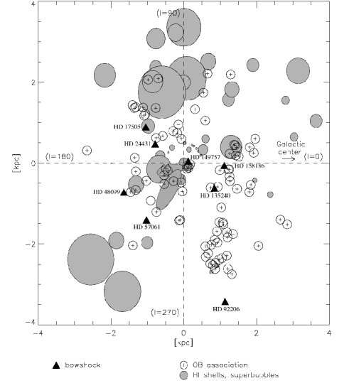
Figure 12: The distribution of the bow shocks in context to superbubbles and OB–associations, as published in Huthoff & Kaper (huthoff (2002)).

6.2 Sample

The distance histogram containing all eight detections is compared to that containing 22 non–detections, without taking into account multiplicity and absorption. The resulting histogram, shown in Fig. 10, reveals that most detections lie within a distance of 2 kpc. This cannot be a result of surface brightness, as it would stay constant with respect to varying distances. The bow shock, or rather the standoff distance, will vary in size when the distance changes. For example HD 92206 is the most distant detection and hence is hardly resolved. Similar results are gained when analysing the velocity histogram in Fig. 11 for the sample. Only bow shocks around slow central stars can be resolved. One can say this sample is complete within 2 kpc and up to velocities of 60 km s^-1.
As described in appendix A, the sample contains only one single system. As for the DES and BSS, only 50% of the created runaways should be multiple systems. Whether more bow shocks are created by multiple systems as for single star systems, or if the fractions of multiples determined from both scenarios is wrong, cannot be stated on the basis of only eight bow shocks.
The location of the eight bow shocks within the galactic plane in Fig. 12 shows that they are not located inside any superbubble. This is to be expected, as the sonic velocity (Eq. 9, with $T\sim 10^{6}$ K) therein would be to high to create a bow shock. Only HD 17505 seems to lie in the superbubble inside GS 137–27–17, which is only an effect of projection. HD 17505 having a $b=-0.9$° lies well above the upper surface of the bubble at $b=0$°. For the three bow shocks with $270\degr\leq l\leq 0\degr$ no data for superbubbles exists.
The typical lifetime of an OB–star with its runaway velocity does not permit it to put a large distance between itself and the OB–association as a probable origin. As shown in Fig. 12 most bow shocks are still near OB–associations, except HD 92206, HD 57061 and HD 17505. The first two, are the fastest stars within the sample, enabling them to move a greater distance, and HD 92206 is also so far away, that OB–associations can only be determined with great difficulty at such a distance. HD 17505 is in the vicinity of a star formation region noted in Carpenter et al. (Carpenter (2000)) not shown in Fig. 12.

7 Conclusion

The search for bow shocks using the H$\alpha$–sample of SHASSA and VTSS yielded eight detections (HD 17505, HD 24430, HD 48099, HD 57061, HD 92206, HD 135240, HD 149757, and HD 158186) from a total of 30 candidates already observed (seven candidates are missing in VTSS), derived from the sample VB used for their search within the IRAS allsky survey.
The best indicator to detect bow shocks within H$\alpha$ images was the correlation between the direction of the proper–motion and the symmetry axis, determined using radial distance profiles, which are not sensitive to bright backgrounds. The other methods can be used for further verification, when in doubt (as for HD 57061).
The detected bow shocks could be successfully used to determine ISM parameters. This was done, either using the standoff distance or the brightness profile. As the sample is only complete up to a distance of 2 kpc and no bow shocks can be found inside a superbubble, the derived values of the density ($\sim 1$ cm^-3) and the maximal temperature ($\sim 10^{4}$ K) fit well to the picture of the WIM (e.g. Shull Shull (1987)). Both features justify the more or less constant ISM density and temperature. Regions of other ISM composition and therefore other parameters, e.g. the regions inside the Small and Large Magellanic Cloud, are too far away and cannot be analysed using the medium resolution of the H$\alpha$–allsky surveys. All in all, bow shocks around OB–runaway stars are ideal probes of the ISM, as are neutron stars (cf. Chatterje & Cordes chatterjee (2002)). They also demonstrate the qualitative picture of the neighbouring ISM is apparently correct.
First steps to clarify the last ambiguity of bubble or bow shock using spectroscopy or velocity charts (see Sect. 6.1) were taken for the eight candidates: Using data from the IUE-archive, absorption profiles of N v, Si iv, and C iv were detected in the case of HD 48099, HD 57060, and HD135240 showing an excess compared to surrounding O–stars and low temperatures of $\sim$15 000 K. As stellar winds are too thin to contribute large amounts of these ions and the temperatures are too low to radiatively excite them, this confirms again these objects as shock fronts of bow shocks. More important, these lines were used to measure the velocities, which fit to the proposed values of the bow–shock layer. Additionally, H i velocity data of HD 17505 from the Canadian Galactic Plane Survey was used to create velocity charts, which showed a velocity distribution as expected in the case of a bow–shock layer. However no data could be found in the literature concerning the other candidates. Hence further spectroscopic analysis of these objects is still needed to make use of the full potential of the current sample as ISM probes.

Appendix A Photometric Data

HD 135240: Penny et al. (Penny (2001)) have determined HD 135240 as a triple system and specified the first component as a O7 III–V, the second as a O9.5 V and the last one as a B0.5 V star. They also measured the UV flux ratios for the different components as $\frac{F_{UV2}}{F_{UV3}}=0.239$ and $\frac{F_{UV3}}{F_{UV1}}=0.179$, so that the magnitudes of the single components could be determined from the total magnitudes given in the SIMBAD–database.
HD 57061: For photometric data, the SIMBAD–database was used and the results of Stickland et al. (Stickland (1996)) of the star being a quintuple system. They could resolve one component as a O9 II star. The other consists of two double systems resulting in a total spectral class of B0.5 V. The single O–star is the dominant star with a ten–times higher flux than the second double binary.
HD 17505: Fabricius & Makarov (Fabricius (2000)) note this star as being a double or triple system and could measure the magnitudes of the brightest component using the Tycho–filtersystem. The spectral class of O9.5 V (Garmany et al. Garmany (1982)) can only be determined for the complete system.
HD 158186: This object was detected as being a variable of the Algol–type by Adelmann et al. (Adelmann (2000)), therefore HD 158186 has to be at least a double system. As the system is not resolved, the star was treated as a single star with photometric data from the SIMBAD–database and the total spectral class of O9.5 V given by Buscombe (Buscomb (1998)).
HD 24431: Fabricius & Makarov (Fabricius (2000)) also analysed this star and classified it at least as a double system and were able to measure the magnitude of two components. As in the case of HD 17505 they used the Tycho–filtersystem. Reed (Reed (1998)) states the spectral class as a O9 IV–V.
HD 92206: The SIMBAD–database notes this star as a double system, but can only give the total magnitude of the system. Therefore it is treated as a single star. Reed (Reed (1998)) could only measure the spectral class of O6, and was not able to determine the luminosity class.
HD 149757: Here the SIMBAD–database notes the star as a single system and its magnitude. The spectral class was measured by Garmany (Garmany (1982)) and is O9 V. Being the nearest star of the eight candidates, the distance determined by Hipparcos could be determined. Both distances are within reasonable agreement with respect to their errors, verifying the spectral parallax results. For consistency, we use the distance determined by spectral parallax.
HD 48099: This star is given as a binary system by Stickland et al. (Stickland (1996)). They could measure the UV–flux ratios for the components as $\frac{F_{UV1}}{F_{UV2}}=1.8$. Garmany (Garmany (1982)) could only determine the total spectral class to O7 V.

References

- (1) Adelman, S. J., Mayer, M. R., & Rosidivito, M. A. 2000, IBVS, 5008, 1
- (2) Blaauw, A. 1961, BAN, 15, 265
- (3) Brown, D. , Bomans, D. J. 2003, ANS, 324, 135B
- (4) van Buren, D. 1983, PhDT, 20
- (5) van Buren, D. 1985, ApJ, 294, 567
- (6) van Buren, D., & McCray, R. 1988, ApJ, 329, L93
- (7) van Buren, D., Noriega–Crespo, A., & Dgani R. 1995, AJ, 110, 2614
- (8) van Buren, D., Mac Low, M.–M., Wood, D.O.S., & Churchwell, E. 1990, ApJ, 353, 570
- (9) Buscombe, W. 1998, yCat, 3206, 0 Carpenter
- (10) Carpenter, J. M., Heyer M. H., & Snell, R. L. 2000, ApJS, 130, 381
- (11) Castor, J., McCray, R., & Weaver, R. 1975, ApJ, 200, L107
- (12) Chatterjee, S., & Cordes, J. M. 2002, ApJ, 575, 407
- (13) Dennison, B., Topasna, G., & Simonetti, J. H. 1997, ApJ, 474, L31
- (14) Evans D. S. 1979, IAUS, 30, 57
- (15) Fabricius, C., & Makarov, V. V. 2000, A&A, 356, 141
- (16) Garmany, C. D., Conti, P. S., & Chiosi C. 1982, ApJ, 263, 777
- (17) Gaensler B. M., Jones D. H., & Stappers B. W. 2002, ApJ, 580, L137
- (18) Gaustad, J. E., McCullough, P. R., Rosing, W., & van Buren, D. 2001, PASP, 113, 1326
- (19) Lamers, H. J. G. L. M., & Cassinelli, J. P. 1999, Introduction to Stellar Winds, Cambridge University Press
- (20) Hoffer, J. B. 1983, AJ, 88, 1420
- (21) Hoogerwerfer, R., de Bruijne, J. H. J., & de Zeuw P. T. 2001, A&A, 365, 49
- (22) Howarth I. D., & Prinja, R. K. 1989, ApJS, 69, 527
- (23) Howarth I. D., Siebert, K. W., Hussain, G. A. J., & Prinja, R. K. 1997, MNRAS, 284, 265
- (24) Huthoff F., & Kaper L. 2002, A&A 383, 999
- (25) Lamers H. J. G. L. M., & Leitherer, C. 1993, ApJ, 412, 771
- (26) Landolt–Börnstein 1982, Astronomy and Astrophysics, Springer, Berlin
- (27) Mac Low, M.–M., van Buren, D., Wood, D. O. S., & Churchwell, E 1991, ApJ, 369, 395
- (28) Hathis, J. S. 1990, ARA&A, 28, 37
- (29) Osterbrock, D.E.O. 1989, Astrophysics of Gaseous Nebulae and Active Galactic Nuclei, University Science Books, Mill Valley
- (30) Panagia, N. 1973, AJ, 78, 929
- (31) Penny, L. R., Seyle, D., & Gies, D. R. et al. 2001, ApJ, 548, 889
- (32) Reed, B. C. 1998, ApJS, 115, 271
- (33) Shull, J. M. 1987, in Proceedings of the Symposium, Interstellar processes, ed D.J. Hollenbach, & H.A. Thronsondr, 225
- (34) Stickland, D. J. 1996, Observatory, 116, 294
- (35) Wilkin, F. P. 1996, ApJ, 459, 377
- (36) Wilson, R. E. 1953, General Catalogue of Stellar Radial Velocities, Carnegie Inst., Washington D.C