GRACOS: Scalable and Load Balanced P³M Cosmological N-body Code

Abstract

We present a parallel implementation of the particle-particle/particle-mesh (P³M) algorithm for distributed memory clusters. The GRACOS (GRAvitational COSmology) code uses a hybrid method for both computation and domain decomposition. Long-range forces are computed using a Fourier transform gravity solver on a regular mesh; the mesh is distributed across parallel processes using a static one-dimensional slab domain decomposition. Short-range forces are computed by direct summation of close pairs; particles are distributed using a dynamic domain decomposition based on a space-filling Hilbert curve. A nearly-optimal method was devised to dynamically repartition the particle distribution so as to maintain load balance even for extremely inhomogeneous mass distributions. Tests using $800^{3}$ simulations on a 40-processor beowulf cluster showed good load balance and scalability up to 80 processes. We discuss the limits on scalability imposed by communication and extreme clustering and suggest how they may be removed by extending our algorithm to include adaptive mesh refinement.

1 Introduction

Cosmological N-body simulations are the main tool used to study the dynamics of collisionless dark matter and its role in the formation of cosmic structure. They first became widely used 20 years ago after it was realized that the gravitational potentials of galaxies are dominated by dark matter. At the same time, theories of the early universe were developed for dark matter fluctuations so that galaxy formation became an initial value problem.

Although many of the most pressing issues of galaxy formation require simulation of gas dynamics as well as gravity, there is still an important role for gravitational N-body simulations in cosmology. Dark matter halos host galaxies and therefore gravitational N-body simulations provide the framework upon which one adds gas dynamics and other physics. Moreover, many questions of structure formation can be addressed with N-body simulations as a good first approximation: the shapes and radial mass profiles of dark matter halos, the rate of merging and its role in halo formation, the effect of dark matter caustics on ultra-small scale structure, etc.

In a cosmological N-body simulation, the matter is discretized into particles that feel only the force of gravity. A subvolume of the universe is sampled in a rectangular (not necessarily cubic) volume with periodic boundary conditions. In principle, one simply uses Newton’s laws to evolve the particles from their initial state of near-perfect Hubble expansion. Gravity takes care of the rest.

In practice, cosmological N-body simulation is difficult because of the vast dynamic range required to adequately model the physics. Gravity knows no scales and the cosmological initial fluctuations have power on all scales. After numerical accuracy and speed, dynamic range is the primary goal of the computational cosmologist. One would like to simulate as many particles as possible (at least $10^{10}$ to sample galaxies well within a supercluster-sized volume), with as great spatial resolution as possible (at least $10^{4}$ per dimension), for as long as possible ($10^{3}$ to $10^{4}$ timesteps to follow the formation and evolution of structure up to the present day).

A single computer is insufficient to achieve the maximum possible dynamic range. One should use many computers cooperating to solve the problem using the technique of parallelization. In a parallel N-body simulation, the computation and memory are distributed among multiple processes running on different nodes (computers). Unfortunately, ordinary compilers cannot effectively parallelize a cosmological N-body simulation code. A programmer must write special code instructing the computers how to divide up the work and specifying the communication between processes.

A parallel code is considered successful if it produces load-balanced and scalable simulations. A simulation is load balanced when the distribution of the effective workloads among the nodes is uniform. Scalability for a given problem means that the wall clock time spent by the computer cluster doing simulations scales inversely with the number of nodes used. Ideally, of course, the code should also be efficient: as much as possible, the wall clock time should be entirely devoted to computation.

At present, there are two main algorithms used for cosmological N-body codes: Tree and P³M (see Bertschinger 1998 for review). The current parallel Tree code implementations include TreeSPH (Davé, Dubinski, & Hernquist, 1997)), HOT (Salmon & Warren, 1994), Gadget (Springel, Yoshida, & White, 2001), and Gasoline (Waldsley, Stadel, & Quinn, 2004). Tree codes have the advantage of relatively easy parallelization and computing costs that scale as $N\log N$ where $N$ is the number of particles. However, they have relatively large memory requirements.

The P³M (particle-particle/particle-mesh) method was introduced to cosmology by Efstathiou & Eastwood (1981) and is described in detail in Efstathiou et al. (1985) (see also Bertschinger & Gelb 1991). For moderate clustering strengths, P³M is faster than the Tree code but it becomes slower when clustering is strong. This is because P³M is a hybrid approach that splits the gravitational force field of each particle into a long-range part computed quickly on a mesh plus a short-range contribution computed by direct summation over close pairs. When clustering is weak, the computation time scales as $N_{\rm gr}\log N_{\rm gr}$ where $N_{\rm gr}\$ is the number of grid (mesh) points, while when clustering is strong the computation time increases in proportion to $N^{2}$. The scaling can be restored to $N\log N$ using adaptive methods (Couchman, 1991).

Currently there exist several parallel implementations of the P³M algorithm, including the version of Ferrell & Bertschinger (1995) for the (now defunct) Connection Machine CM-5 and the Hydra code of MacFarland et al. (1998). The Hydra code uses shared memory communications for the Cray T3E. There is a need for a message-passing based version of P³M (and its adaptive extension) to run on beowulf clusters. This need motivates the present work.

The difficulty of parallelizing adaptive P³M has led a number of groups to use other techniques to add short-range forces to the particle-mesh (PM) algorithm. The Tree and PM algorithms have been combined by Bode & Ostriker (2003) and Dubinski et al. (2004) while Merz, Pen, & Trac (2004) use a two-level adaptive mesh refinement of the PM force calculation. The FLASH code (Fryxell et al., 2000) has been extended to incorporate PM forces with multi-level adaptive mesh refinement.

When the matter distribution becomes strongly clustered, parallel codes based on PM and P³M face severe challenges to remain load-balanced.

In general, P³M and PM-based parallel codes suffer complications when the matter becomes very clustered as happens at the late stages of structure formation. Most of the existing codes use a static one-dimensional slab domain decomposition, which is to say that the simulation volume is divided into slices and each process works on the same slice throughout, even when the particle distribution becomes strongly inhomogeneous. The GOTPM code uses dynamic domain decomposition, with the slices changing in thickness as the simulation proceeds, resulting in superior load balancing. However, even this code will break down at very strong clustering because it also uses a one-dimensional slab domain decomposition. The FLASH code uses a more sophisticated domain decomposition similar in some respects to the method introduced in the current paper.

The motivation of the current work is to produce a publicly available code that will load balance and scale effectively for all stages of clustering on any number of nodes in a beowulf cluster. This paper introduces a new, scalable and load-balanced approach to the parallelization technique for the P³M force calculation. We achieve this by using dynamic domain decomposition based on a space-filling Hilbert curve and by optimizing data storage and communication in ways that we describe.

This paper is the first of two describing our parallelization of an adaptive P³M algorithm. The current paper describes the domain decomposition and other issues associated with parallel P³M. The second paper will describe the adaptive refinement method used to speed up the short-range force calculation.

The outline of this paper is as follows. The serial P³M algorithm (based on Gelb & Bertschinger 1994 and Ferrell & Bertschinger 1994) that underlies our parallelization is summarized in §2. Section 3 discusses domain decomposition methods starting with the widely-implemented static one-dimensional slab decomposition method. We then introduce the space-filling Hilbert curve and describe its use to achieve a flexible three-dimensional decomposition. Section 4 presents our algorithm for dynamically changing the domain decomposition so as to achieve load balance. Section 5 presents our techniques for organizing the particle data so as to minimize efficiency in memory usage, cache memory access, and interprocessor communications. In §6 we describe the algorithms used to parallelize the PM and PP force calculations. Section 7 presents code tests emphasizing load balance and scalability. Conclusions are presented in §8. An appendix presents an overview of the code and frequently appearing symbols, and another appendix briefly describe the routines used to map the Hilbert curve onto a three-dimensional mesh and vice versa.

2 Serial P³M C-code and force calculation

In this section we summarize our serial cosmological N-body C implementation p3m based on an earlier serial Fortran implementation of P³M by one of the authors. We discuss in detail the code units and aspects of the force calculation that are necessary for understanding the parallelization issues covered in the later sections.

2.1 Long and Short Range Forces and the Pairwise Force Law

Given the pairwise force ${\bf F_{0}}({\bf r}_{12})$ between two particles of masses $m_{1}$ and $m_{2}$ and separation ${\bf r}_{12}={\bf x}_{2}-{\bf x}_{1}$, we define the interparticle force law profile ${\bf\Theta}_{0}({\bf r})\equiv{\bf F_{0}}({\bf r}_{12})/(Gm_{1}m_{2})$. For a system of many particles, the gravitational acceleration of particle $i$ is $\sum_{j\neq i}Gm_{j}{\bf\Theta}_{0}({\bf r}_{ij})$.

The required interparticle force law profile depends on the shape of the simulation particles. For point particles one uses the inverse square force law profile ${\bf\Theta}_{0}({\bf r})=-{\bf r}/r^{3}$. The inverse square force law is not used for simulation of dark matter particles in order to avoid the formation of unphysical tight binaries, which happens as a result of two-body relaxation (Binney & Tremaine, 1994). For cold dark matter simulations many authors use the Plummer (1911) force law

$${\bf\Theta}_{\rm PL}({\bf r},\epsilon)\equiv-\frac{\bf r}{(r^{2}+\epsilon^{2})^{3/2}}\ ,$$ (1)

where $\epsilon$ is the Plummer softening length. We take the Plummer softening length to be constant in comoving coordinates. With Plummer softening the particles have effective size $\epsilon$. In a P³M code, $\epsilon$ is usually set to a fraction of the PM-mesh spacing.

In a P³M code, the desired (e.g., Plummer) force law is approximated by the sum of a long-range (particle-mesh or PM) force evaluated using a grid and a short-range (particle-particle or PP) force evaluated by direct summation over close pairs. The PM force ${\bf\Theta}_{\rm PM}({\bf x}_{i},{\bf x}_{j})$ varies slightly depending on the locations of the particles relative to the grid (see Appendix A of Ferrell & Bertschinger 1994). The average PM force law $\langle{\bf\Theta}_{\rm PM}\rangle({\bf r}_{ij})$ can be tabulated by a set of Monte-carlo PM-force simulations each having one massive particle surrounded by randomly placed test particles (Bertschinger, 1991). In practice, the mean PM force differs from the inverse square law by less than 1% for pair separations greater than a few PM grid spacings. For smaller separations, a correction (the PP force) must be applied. The total force is given by

$${\bf\Theta}_{\rm P3M}({\bf r}_{ij})\equiv{\bf\Theta}_{\rm PP}({\bf r}_{ij})+{\bf\Theta}_{\rm PM}({\bf x}_{i},{\bf x}_{j})\ .$$ (2)

Strictly speaking, the P³M force is not translationally invariant and therefore depends on the positions of both particles. The P³M force differs from the exact desired interparticle force profile ${\bf\Theta_{0}}$ by ${\bf\Theta}_{\rm Error}({\bf x}_{i},{\bf x}_{j})\equiv{\bf\Theta}_{\rm P3M}({\bf x}_{i},{\bf x}_{j})-{\bf\Theta_{0}}({\bf r}_{ij})={\bf\Theta}_{\rm PM}({\bf x}_{i},{\bf x}_{j})-\langle{\bf\Theta}_{\rm PM}\rangle({\bf r}_{ij})$.

At large separations, both the PM-force and the required force reduce to the inverse square law (modified on the scale of the simulation volume by periodic boundary conditions). The PP-force can therefore be set to zero at $r\geq R_{\rm max}$ for some $R_{\rm max}$. The PP-correction is applied only for separations $r<R_{\rm max}$. The PM-force on the other hand is mainly contributed by remote particles.

2.2 Dynamic Equations and Code Units

The equation of motion of particles in a Robertson-Walker Universe is

$$\frac{d^{2}\bf x}{d\tau^{2}}+\frac{1}{a}\frac{da}{d\tau}\frac{d\bf x}{d\tau}=-\nabla_{\bf x}\phi\ ,$$ (3)

where ${\bf x}\equiv\{x^{0},x^{1},x^{2}\}$ is the comoving position and $\tau$ is comoving (conformal) time. The potential $\phi$ satisfies the Poisson equation

$$\nabla_{\bf x}^{2}\phi=4\pi Ga^{2}\delta\rho\,({\bf x},\tau)\ ,$$ (4)

where $\delta\rho$ is the excess of the proper density over the background uniform density.

The equations take a simpler and dimensionless form in a special set of units that we adopt. The coordinates, energy and time in our code are brought to this form. Let us denote by tildes variables expressed in code units. Then for the units of time, position, velocity and energy (or potential), we write $d\tilde{t}=H_{0}dt/a^{2}=H_{0}d\tau/a$, $\tilde{x}=x/\Delta x$, $\tilde{v}=v(a/H_{0}\Delta x)$ and $\tilde{E}=E(a/H_{0}\Delta x)^{2}$ or $\tilde{\phi}=\phi(a/H_{0}\Delta x)^{2}$, where $a$ is the expansion factor of the universe, $v$ is the proper velocity, $H_{0}$ is the Hubble constant and $\Delta x$ is the cell spacing of the PM density mesh in our code (see Sec. 2.5) expressed in comoving Mpc. In these units, the equation of motion (3) reduces to

$$\frac{d\tilde{\bf x}}{d\tilde{t}}=\tilde{\bf v}\ ,\ \ \frac{d\tilde{\bf v}}{d\tilde{t}}=\tilde{\bf g}\equiv\tilde{m}\tilde{\bf\Theta}({\bf r})=-\nabla_{\bf{\tilde{x}}}\tilde{\phi}\ .$$ (5)

We choose units of mass so that the Poisson equation takes the following form in dimensionless variables:

$$\nabla_{\tilde{\bf x}}^{2}\tilde{\phi}=\frac{3\Omega_{m}a}{2}\delta\tilde{\rho}\ ,\ \ \delta\tilde{\rho}\equiv\delta\rho/\bar{\rho}_{m}\ ,$$ (6)

where $\bar{\rho}_{m}=3\Omega_{m}H_{0}^{2}/(8\pi G)$ is the proper mean matter density. Particle masses are made dimensionless by $\tilde{m}=m/[\bar{\rho}_{m}(a\Delta x)^{3}]$. The dimensionless total mass of all the particles is ${\tilde{M}}_{\rm tot}=N_{\rm gr}$ where $N_{\rm gr}$ is the total number of PM mesh points. Periodic boundary conditions are assumed in each dimension so that a finite volume simulation represents a small portion of a universe that is homogeneous on larger scales.

As a check on overall code accuracy, we monitor global energy conservation by integrating the Layzer-Irvine equation, which in code units takes the form

$$\frac{d}{d\tilde{t}}\,(\tilde{E}_{k}+\tilde{E}_{g})=\frac{\tilde{E}_{g}}{a}\frac{da}{d\tilde{t}}\;,$$ (7)

where

$$\tilde{E}_{g}\equiv-\frac{1}{2N_{\rm gr}}\sum_{i,j}\tilde{m}_{i}\tilde{m}_{j}\int^{\infty}_{r_{ij}}{\tilde{\bf\Theta}}(r)\,dr\ \ \mbox{and}\ \ \tilde{E}_{k}\equiv\frac{1}{N_{\rm gr}}\sum_{i}\frac{\tilde{m}_{i}\tilde{v}_{i}^{2}}{2}$$ (8)

are the dimensionless gravitational and kinetic energies in the simulation. Note that in a Robertson-Walker background, the Hamiltonian is time-dependent and so the energy is not conserved (Bertschinger, 1996). However, we can integrate equation (8) to get a quantity that should remain constant as the simulation progresses,

$$\tilde{E}_{\rm con}\equiv\int\,d\tilde{E_{k}}+\int\,d\tilde{E_{g}}-\int\tilde{E_{g}}\,d\ln{a}\;.$$ (9)

2.3 Particle Data Structure and Layout

A particle is represented in both our serial and parallel codes by a structure, defined as

$${\tt typedef\ struct\ part\_t\ \{float\ x0,x1,x2,mass,g0,g1,g2;}$$

$$\quad\quad\quad\quad\quad\quad\quad\quad\quad\quad\quad\ \ {\tt int\ id;\ float\ v0,v1,v2;\}\ part\_t}\ .$$ (10)

The size of the structure is 44 bytes on 32 bit machines. The structure contains three positions, the mass, accelerations and velocities of the particles along the three spatial Cartesian directions, all made dimensionless by the choice of units described above. In addition, the integer ${\tt id}$ is used to tag particles. This number can be arbitrary and is not used anywhere in force calculations or particle propagation. In the serial code, the particles are stored in memory simply as an array with base pointer ${\tt pa}$ and end pointer ${\tt pa\_f}={\tt pa}+N,$ where $N$ is the total number of particles in the simulation volume. To scan all the particles, e.g. for their imaging, we loop over all the pointers ${\tt p}$ within the range ${\tt p\in[\,{\tt pa},{\tt pa\_f})}$. The particle masses are not required to be equal to each other in general.

2.4 Particle Integration and Timestep Criterion

All the particles in the code are positioned within the simulation box of size $L^{i}=n^{i}\Delta x$, where $i\in\{0,1,2\}$ labels the spatial dimension. (We allow for unequal lengths with $n^{i}/n^{j}$ equalling a ratio of small integers.) Periodic boundary conditions are applied to bring particles that move outside back into the simulation volume. We currently use a Drift-Kick-Drift (DKD) leapfrog integrator scheme (Ruth, 1983; Saha & Tremaine, 1992) to integrate the equations of motion (5) for the particles:

$$\begin{array}[]{l}{\bf x}_{n+1/2}={\bf x}_{n}+\frac{1}{2}{{\bf v}_{n}\,\Delta t}\\[3.0pt] {\rm Force\;calculation\;}{\bf g}_{n+1/2}\\[3.0pt] {\bf v}_{n+1}={\bf v}_{n}+{\bf g}_{n+1/2}\,\Delta t\\[1.0pt] {\bf x}_{n+1}={\bf x}_{n+1/2}+\frac{1}{2}{{\bf v}_{n+1}\,\Delta t}\ ,\end{array}$$ (11)

where the subscripts denote timesteps. Hockney & Eastwood (1988) discuss the accuracy and stability of this scheme. Note that the P³M force calculation is needed only once each timestep.

All integrators have advantages and limitations. For our problem, which can be expressed as a continuum Hamiltonian time evolution, the leapfrog integrator of equation (11) is a good choice, since with a constant timestep it is symplectic. A symplectic integrator preserves the Poincaré integral invariants and follows the time evolution under a discrete Hamiltonian that is close to the continuum Hamiltonian of interest. The difference between the discrete and continuum Hamiltonian or the discrete integrator error is itself a Hamiltonian. When the error is a Hamiltonian, and is sufficiently small, according to the KAM theorem (Arnold, 1978) the difference between the Hamiltonian paths evolved by the two Hamiltonians is a set of finite measure. Therefore most of the structure of the Hamiltonian flow evolved by the continuum Hamiltonian will be preserved when evolved by the discrete Hamiltonian with the symplectic integrator. Most of the stable orbits in the continuum Hamiltonian system will remain stable under the discrete Hamiltonian evolution and vice versa.

Higher order symplectic integrators for Hamiltonian evolution can be constructed using the method of Yoshida (1990), which requires more force evaluations per timestep. In general, a $N$-th order symplectic integrator requires at least $N-1$ force evaluations per complete timestep.

In a cosmological simulation, particles become more clustered with time. It is not practical therefore to have a fixed value of the timestep for the whole simulation. Currently we advance equation (11) with the same value of timestep $\Delta t$ for all the particles but allow it to change with time. The choice for $\Delta t$ is based on the current particle data and therefore depends on the phase space variables. Consequently, equation (11) is no longer an exact symplectic map. Nevertheless, it remains in practice well-behaved provided the timestep varies sufficiently slowly.

The timestep must at least satisfy the leapfrog stability criterion $(da/dx)_{\max}(\Delta t)^{2}<4$ given by equation (4-42) of Hockney & Eastwood (1988). This stability requirement is essentially equivalent to the constraint that the global timestep must be small enough not to exceed the local dynamical time at any point within the simulation box, $\Delta t\sim\sqrt{\eta_{t}/(G\rho_{\max})}$ where $\eta_{t}$ is a dimensionless constant. The density is somewhat expensive to obtain, but given the particle accelerations and using the approximation $g\sim GM/r^{2}\sim G\rho r^{3}/r^{2}\sim G\rho\epsilon$, we have now, expressed in code units,

$$\Delta\tilde{t}=\sqrt{\frac{\eta_{t}\,\tilde{\epsilon}}{\tilde{g}_{\max}}}\ ,$$ (12)

where $\tilde{\epsilon}$ is the dimensionless Plummer softening length (see § 2.1), $\eta_{t}$ is a free parameter in the code usually set to a small value such as $\eta_{t}=0.05$, and $\tilde{g}_{\rm max}$ is the maximum acceleration of a particle in the simulation box in code units. This criterion is conservative in assuring that the orbits of all particles are well sampled.

To further improve the integration technique, one may consider adaptive integrators, with individual particle timesteps changing according to the local dynamical time at the given position within the simulation volume (Quinn et al., 1997). On the other hand, one may consider higher order symplectic integrators, which would require more force evaluations per timestep. Some of the non-symplectic higher order integrators, such as Runge-Kutta, are known not to preserve the Hamiltonian flow structure even with fixed timesteps. For example, it can be shown by integration of Kepler orbit that the popular fourth order Runge-Kutta integrator yields a divergent orbit very quickly. On the other hand, for second order integrators, the DKD scheme shows stable orbits with errors behaving as small perturbations as expected on the basis of KAM theorem.

In this paper we adopt the leapfrog integrator with variable timestep (set to the same value for all particles), leaving the implementation of a higher order symplectic integrator and individual particle timesteps for future work.

2.5 Particle-Mesh Force Calculation

The particle–mesh (PM) force is the long-range force that can be computed using Fast Fourier Transforms (FFT). In our code, we use the FFTW Fourier transform implementation (Frigo & Johnson, 2003) and the PM algorithm of Ferrell & Bertschinger (1994). For large total number of particles $N$ in the simulation box, the PM force computation is faster than the direct summation method, requiring only $\propto N_{\rm gr}\log{N_{\rm gr}}$ operations in total ($N_{\rm gr}\equiv n^{0}n^{1}n^{2}$ is the number of PM grid points), as opposed to $O(N^{2})$.

The rectangular PM-density mesh is allocated for the whole simulation volume in the serial code. This grid is to be filled with the density values interpolated from the particles nearby. Hockney & Eastwood (1988) discuss a number of methods for the density interpolation with increasing smoothness, ranging from Nearest Grid Point (NGP) to Cloud-in-Cell (CIC) to the Triangular-Shaped Cloud (TSC) method. The highest of accuracy of these is given by the TSC interpolation scheme and that is the scheme we have implemented. As shown by Hockney & Eastwood (1988), an interpolation of the mass value from a particle at position $\tilde{\bf x}$ to a grid point at position $\tilde{\bf x}_{\rm gr}$ within the PM mesh and vice versa takes place if and only if

$$\max\limits_{i=\{0,1,2\}}\left|\tilde{x}^{i}-\tilde{x}^{i}_{\rm gr}\right|\leq{L_{\rm SCH}}\ ,$$ (13)

where the absolute value is taken with the proper account for the boundary conditions, and ${L_{\rm SCH}}$ is the window function domain locality length, specific to the interpolation scheme used, e.g. $L_{\rm NGP}=\frac{1}{2}$, $L_{\rm CIC}=1$ and $L_{\rm TSC}=\frac{3}{2}$. In our code we have ${L_{\rm SCH}}=L_{\rm TSC}$.

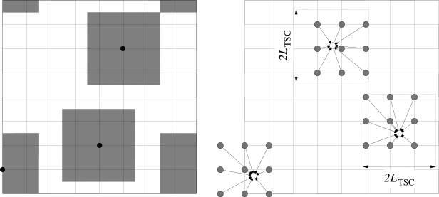
Figure 1: Left: Density interpolation from particles to grid points PM Step 1. To interpolate the density to a given grid point one needs to add contributions from all of the particles inside the shaded box of length $2L_{\rm TSC}$ centered on the grid point. Right: force interpolation from grid points to particles PM Step 5. To get the force on a given particle (open circle), force values are used from all of the surrounding grid points.

There are several steps involved for one PM force calculation:

1. Density interpolation: Masses of particles are interpolated to a rectangular density mesh of grid points using a forward TSC interpolation scheme as illustrated by the left Figure 1. Details are given on pp. 142–146 of Hockney & Eastwood (1988) and equation (A.16) of Ferrell & Bertschinger (1994).

2. The mesh density is Fourier transformed to the complex domain.

3. The force is computed in the complex domain using a pretabulated Green’s function given by equation (A.14) of Ferrell & Bertschinger (1994).

4. The mesh force field is inversely Fourier transformed to return to the real domain.

5. Force interpolation: Forces are interpolated from the force mesh to particles using a backward TSC interpolation scheme, as shown in the right Figure 1. This step is opposite to Step 1.

In Step 5, information flows in exactly the opposite direction as Step 1. Only the same grid points satisfying equation (13) that acquired their density values from the particles in Step 1 are used for the interpolation of the forces to only the same particles in Step 5. If an exchange of the information between a grid point and a particle ever occurs, it has to be both ways. This point will be very useful when we discuss density and force grid messages for the parallel code in §6.1.2.

The timing of the PM force evaluation scales as

$$t_{\rm PM}\propto A\,N+B\,N_{\rm gr}\log(N_{\rm gr})\ ,$$ (14)

where the first term is due to the density and force interpolation and the second is due to the Fast Fourier Transform. The coefficients $A$ and $B$ do not depend on $N$ and $N_{\rm gr}$. The coefficient $A$ depends on the interpolation scheme used. For the TSC interpolation scheme in $d=3$ dimensions, the density is always interpolated from a particle to the $(2L_{\rm TSC})^{d}=27$ nearby grid points satisfying the condition (13). During the force interpolation, the inverse occurs three times: once for each of the three spatial dimensions. The factor of $4\times 27$ therefore enters into an expression for $A$ when TSC interpolation is used. The coefficient $B$ is independent of $A$ and is given by the existing benchmarks for the FFTW implementation (Frigo & Johnson, 2003).

2.6 PP Force Calculation and the Chaining Mesh

In order to calculate the short range force, we must first find all the pairs separated by less than $\tilde{R}_{\max}$. This is accomplished using a fast linked-list sorting procedure (Hockney & Eastwood, 1988). At the start of a simulation the whole simulation volume is partitioned into rectangular chaining mesh cells whose spacings in dimension $i$ are constrained by

$$\Delta\tilde{x}_{c}^{i}\geq\tilde{R}_{\max}\ .$$ (15)

Given this constraint, for any particle in any chaining mesh cell, only the particles within the same or one of the adjacent chaining mesh cells need be included in the short range force calculation, since the PP force is zero for separations greater than $\tilde{R}_{\max}$. Choosing the smallest possible value satisfying equation (15), this leads to

$$\Delta\tilde{x}_{c}^{i}=\frac{\tilde{L}^{i}}{n_{c}^{i}}\ ,\ \ \mbox{where}\ \ n_{c}^{i}=\left[\,{\tilde{L}}^{i}/\tilde{R}_{\max}\right]\ ,$$ (16)

where the square brackets signify taking the integer part. At the start of the run, we sort all the particles into chaining mesh cells occupying the 3D volume and form linked lists of particles belonging to each cell. Each chaining mesh cell then contains the root of the linked list to all the particles within that cell.

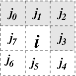
Figure 2: The cells $j_{0}\ldots j_{3}$ constitute the 4 cells needed for PP force calculation in two dimensions, $B^{\rm PP}=\{j_{0},j_{1},j_{2},j_{3}\}$.

In order to apply a short range force correction to a particle $p$ within the simulation volume, we access particles contained within the same cell as well as the particles within the $3^{d}-1=26$ surrounding chaining mesh cells. Since the short range correction procedure is applied for each pair of particles within the simulation volume, we need to traverse only half of the surrounding cells, as illustrated in Figure 2. For a given chaining mesh cell $j$, let $N_{\rm CM}(j)$ be the number of particles within the cell and $B^{\rm PP}(j)$ be the set of the $(3^{d}-1)/2$ surrounding cells used for the short range force calculation. The number of floating point operations needed in order to apply the short range force correction for every particle within the simulation volume scales as

$$t_{\rm PP}\propto\sum_{j}N_{\rm CM}(j)\;\left[\frac{1}{2}N_{\rm CM}(j)+\sum_{j^{\prime}\in B^{\rm PP}}N_{\rm CM}(j\,^{\prime})\right]\ .$$ (17)

The PP force calculation takes a lot of time when particles are highly clustered because of the quadratic dependence on numbers.

2.7 Memory requirements

	Memory size	Memory size, for a $32^{3}$ P3M simulation, in bytes.
Particle array	$4\,\hbox{bytes}\times 11N$	1,441,792
Particle linked list	$4\,\hbox{bytes}\times 2N$	262,144
Chaining mesh	$4\,\hbox{bytes}\times n_{c}^{0}n_{c}^{1}n_{c}^{2}$	5,324
Green’s function	$4\,\hbox{bytes}\times n^{0}n^{1}(n^{2}/2+1)$	69,632
Density and Force meshes	$4\,\hbox{bytes}\times 2\times n^{0}n^{1}(n^{2}+2)$	278,528
Total	$4\,\hbox{bytes}\times(13N+\newline 5n^{0}n^{1}(n^{2}/2+1)+n_{c}^{0}n_{c}^{1}n_{c}^{2})$	2,057,420

Table 1: Dominant memory requirements of the serial p3m code

The total memory requirement for the serial code consists of several significant parts listed in Table 1, where the variables $n^{i},n_{c}^{i}$ and $N$ are defined in Table 5 of Appendix A. Using the serial N-body code with an average of $p$ particles per PM gridpoint, the total memory requirement for a P³M code is

$$M_{\rm tot}=\left(13p+\frac{5}{2}+\frac{1}{\tilde{R}_{\max}^{3}}\right)n^{0}n^{1}n^{2}\times 4\ \mbox{bytes}$$

The maximum amount of memory available for dynamic allocation for a 32-bit machine in Unix is 2 GB. In practice the amount of memory available for our application is about 30% smaller. For a simulation having one particle per density mesh cell with a cubic grid, $M_{\rm tot}=(31/2)\,N_{\rm gr}^{3}\times 4$ bytes. The maximum problem size for such a simulation with the upper limit on total memory of $1.4$Gb is $N_{\rm gr}=296^{3}$. This severe limitation on problem size is avoided using the parallel code described in the rest of this paper.

3 Hilbert Curve Domain Decomposition

In order to perform simulations with more than $296^{3}$ particles and gridpoints, we distribute the computation to multiple processors of a parallel computer. We are using the Single Program, Multiple Data (SPMD) model in which one program runs on multiple processors which perform computations on different subsets of the data. The first decision to be made is how to distribute the data and computation. The computational volume is divided into parts called domains and the memory and computation associated with each domain is assigned to a different parallel process.

The problem of domain decomposition is to decide how to partition the computational volume into domains. As we will see, there are a number of considerations that enter this decision. This section first describes the simplest method, one-dimensional static domain decomposition, which is well suited for spatially homogeneous problems but not for strongly clustered N-body simulations. We then introduce the Hilbert curve method of dynamic domain decomposition used in our parallel code.

We use the word process to refer to one of the instances of our parallel program being applied to the data in its domain. A process may correspond to one CPU (or one virtual CPU, in the case of hyperthreading) or there may be multiple processes on one CPU.

3.1 Static Slab Domain Decomposition

In a static slab domain decomposition, the volume is divided by fixed planes with equal spacing. This it the method used, for example, in the FFTW Fast Fourier Transform (Frigo & Johnson, 2003). It is well suited for problems in which the computation is uniformly distributed over volume. A variation on this method is to use a two-dimensional lattice of columns instead of a one-dimensional lattice of slabs.

Several groups have implemented static domain decomposition in parallel N-body codes based on PM or P³M (see §1). As a first step, we developed our own implementation llpm-sl of the static slab domain decomposition Particle-Mesh N-body code.

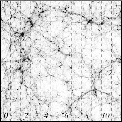
Figure 3: Sample particle distribution with 12 computing processes and a static slab domain decomposition. Processes 1, 2, 3, 8, and 9 have significantly more particles than the others.

A static slab or any other static particle domain decomposition is a good strategy when the number density distribution of particles across the simulation box is nearly uniform and each slab contains approximately the same number of particles to process each timestep. However, gravitational instability destroys the spatial uniformity leading to serious inefficiency. As particle clusters grow, the memory and computational resources of the processes containing the largest clusters (e.g. processes 1, 2, 3, 8, and 9 in Figure 3) grow quickly. Other processes finish their work and have to wait idle. Worse, the heavily loaded processes may run out of memory causing paging to disk. The inevitable result is that the computation becomes unbalanced and the code grinds to a halt (see the timing results in §7 for a $512^{3}$ test run). The same problem will arise in any gravitational N-body code that uses static domain decomposition.

Such a situation, when the performance of the cluster degrades as a result of hugely varying workloads, is called work load imbalance. In the remainder of this section we introduce an alternative method of dynamic domain decomposition that solves the load imbalance problem for strongly clustered systems.

3.2 Dynamic Domain Decomposition with a Hilbert Curve

As we have seen from the slab domain decomposition example in the previous section, it is important for an N-body code to load balance. We solve the load balancing problem by the implementation of dynamic particle domain decomposition defined by a Hilbert space-filling curve as suggested by Pilkington & Baden (1996). Domain decomposition methods based on Morton ordering (a different space-filling curve) have been used by Salmon & Warren (1994) and Fryxell et al. (2000).

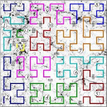
Figure 4: The same matter distribution as in Fig. 3, but now superimposed by a Hilbert curve. The Hilbert curve is divided into 12 colored segments separated by cross-hatched bars and labelled by the circled numbers. During the run the partitions will move along the Hilbert curve so that each process will have approximately the same amount of work to do. In a real simulation the Hilbert curve is divided into much finer segments.

The Hilbert curve (HC) is a fractal invented by the German mathematician in 1891 and is one of the possible space-filling curves that completely fill a cubic rectangular volume. A unique HC is defined for any positive integer $m$ (the HC order), and dimensionality $d$, for which the HC will fill each cell of a $d$-dimensional cube of length $2^{m}$. For $d=2$, examples are given in Figures 4 (with $m=4$) and 5 (with $m=3$). The HC provides a bijective (one-to-one) mapping between the index $h$ along the curve (the HC index) and the cell within the volume. In our code the mapping was provided by the Hilbert curve implementation of Moore (1994) (see Appendix B). The real simulation volume and the space filling curve we use are in fact three-dimensional but the two-dimensional case is used in the figures throughout the paper in order to simplify the presentation.

The main idea of Hilbert curve domain decomposition is to take a three-dimensional volume with inhomogeneous workload and to convert it into a one-dimensional curve that is easily partitioned into approximately equal workloads. The key advantage compared with slab decomposition is that the Hilbert curve method breaks up the problem into $2^{md}$ chunks of work with $d=3$ instead of $d=1$. With much finer granularity it is possible to load balance extremely inhomogeneous problems. In addition, the Hilbert curve minimizes communication between processes, as we show below.

The Hilbert curve has the following properties:
${\it 1)}$ Compactness: it tends to fill the space very compactly. A set of cells defined by a continuous section of a HC tends to be quasi-spherical, having small surface to volume ratio. One can approximate the surface to volume ratio of any continuous segment of $n$ cells along the three-dimensional Hilbert curve with

$$\mbox{S.V.R.}(n)\approx\frac{4.8}{n^{1/3}}\ ,$$ (18)

which decreases with the increasing $n$. This approximation is crude at small $n$. The maximum possible ratio $\mbox{S.V.R.}(1)=26$ is reached for $n=1$, since one volume cell is surrounded by 26 adjacent surface cells.
${\it 2)}$ Locality: the successive cells along the curve are mapped next to each other within the mesh;
${\it 3)}$ Self-similarity: the curve is self-similar on different scales. It can therefore be extended to arbitrarily large size.

Figure 4 demonstrates the bijective mapping of $16\times 16$ cells in a two-dimensional computational volume onto the indexed Hilbert space-filling curve. The curve visits each cell of the simulation volume exactly once. By connecting the two ends of the curve, the curve has the topology of a circle. By introducing $n_{\rm pr}$ partitions along the circle (the partitioning state) each being ascribed to one of the $n_{\rm pr}$ processes in the parallel code, we specify the particle domain decomposition of the whole simulation volume into $n_{\rm pr}$ Local Regions, each consisting of the cells along the curve between two adjacent partitions and being assigned to one of the $n_{\rm pr}$ processes. Let us denote the local region of process $i$ defined by the partitioning state and the Hilbert curve by $L_{h}^{i}$.

As we see, the space-filling curve provides an easy way of bookkeeping for decomposition, since the local domains of each process are completely specified by the Hilbert curve setup and the $n_{\rm pr}$ numbers that specify the partitioning state.

The surface to volume ratio of local domains defined by the continuous segments of the Hilbert curve is small due to the compactness property of the Hilbert curve. This is the primary reason for choosing a Hilbert curve as the space filling curve for our domain decomposition. The small surface to volume ratio significantly speeds up the reassignment of particles crossing the $L_{h}$ boundaries (§ 5.1) and the PP-force computation (§ 6.3). In the $N=800^{3}$ run presented in §7.3, the surface to volume ratio was on average $0.1$ for the domains of voids. In the Hydra code (MacFarland et al., 1998), using a static $7\times 7$ two-dimensional cyclic domain decomposition, the surface to volume ratio is $(4\times 7)/(7^{2})\approx 57\%$, leading to more than five times as much communication cost for the particle advancement and the PP-calculation in comparison to our algorithm.

3.3 Hilbert Curve Initialization

At the beginning of a simulation we set up the Hilbert curve completely using the functions of Moore (1994) with an appropriate choice of the HC mesh parameters. Only one parameter, the Hilbert curve order $m$, is needed to completely specify the geometry of a Hilbert curve filling an entire $d$-dimensional cube of volume $(2^{m})^{d}$, which we will call the complete HC-mesh. Adding more parameters — the HC mesh cell spacings $dx_{h}^{i}\,,\,i\in\{1,2,3\}$, the curve starting point in the simulation volume, and the curve orientation — completely determines the Hilbert curve within the simulation volume.

While the real N-body simulation volume and the space filling curve are three dimensional, two dimensional examples are used in figures throughout this paper solely to simplify the presentation.

We use the Hilbert curve in our code only to specify the domain decomposition for particle storage and computation. The domain decomposition does not affect any physical values computed. The choice of the Hilbert curve order $m$ in our code is made based solely on the parallel code performance considerations. From the point of view of improving the resolution for particle domain decomposition, higher $m$ is preferred. On the other hand each local region cell costs additional memory, favoring lower $m$. For a P³M simulation, in order to simplify the force calculation, we choose the HC mesh cells to coincide with the PP chaining mesh cells:

$$\Delta\tilde{x}_{h}^{i}\equiv\Delta\tilde{x}_{c}^{i}\ ,\quad n_{h}^{i}\equiv n_{c}^{i}\ .$$ (19)

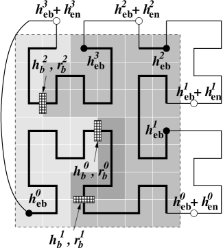
Figure 5: Structure of the domain decomposition. A two-dimensional Hilbert curve (solid line) of order $m=3$ fills a $6dx_{h}^{0}\times 7dx_{h}^{1}$ simulation box (dashed line). By connecting the ends of the Hilbert curve, the resulting curve has a circular topology. The number of processes is $n_{\rm pr}=3$, so there are 3 partitions along the circle indicated by the cross-hatched bars. We have $h_{\rm b}^{i}=\{11,14,58\}$, $h_{\rm n}^{i}=\{3,44,17\}$ and $r_{\rm b}^{i}=\{11,14,38\}$, $r_{\rm n}^{i}=\{3,24,15\}$.

While the complete HC-mesh is a cube of length $2^{m}$ cells, the chaining mesh length does not have to be a power of two. Therefore we choose the HC order $m$ to be the smallest integer satisfying

$$2^{m}\geq n_{h}^{i}\ ,\quad i=\{x,y,z\}\ .$$ (20)

From equations (19) and (20), the complete chaining mesh is just a subset of the complete HC mesh. If $n_{h}^{i}=2^{m}$ for all $i=0\ldots(d-1)$, as in Figure 4, the curve completely fits the simulation volume and the two coincide. If $2^{m}>n_{h}^{i}$ for some $i$, the complete Hilbert curve mesh covers an extra space outside the chaining mesh of the simulation volume as in Figure 5, containing the chaining mesh as a subset. We will refer to this submesh as the Simulation Volume HC mesh or simply as the Hilbert curve mesh where the context is clear.

Since the cells of the HC outside the simulation volume are irrelevant, they do not take memory and their HC indices are irrelevant too. Let us introduce a raw HC index along the curve. For a HC mesh cell ${\bf c}$ which belongs to the simulation volume, we define the raw HC index r, $r\in[0,n_{h}^{0}n_{h}^{1}n_{h}^{2})$, as the number of HC cells that the curve spent within the simulation volume since its starting point (HC index $h=0$). In other words, while the HC index is incremented each cell along the curve, the HC raw index is incremented only at the cells along the curve that belong to the simulation volume.

The mapping between the HC index $h$ and the HC raw index $r$ is specified completely by the table of HC entries. Each entry contains the HC index of an entry point $h_{\rm eb}^{k}$ of the curve into the simulation volume and the number of consecutive HC cells that the HC spends within the simulation volume $h_{\rm en}^{k}$ before the next exit. Let $K$ be the number of entries in the HC table, and let $K\equiv 1$ if the HC mesh fits the simulation box exactly [$n_{h}^{i}=2^{m}$ for each $i=0\ldots(d-1)$]. Because the Hilbert curve visits all the cells in the simulation box, we have

$$n_{h}^{0}n_{h}^{1}n_{h}^{2}=\sum\limits_{k=0}^{K-1}h_{\rm en}^{k}\ .$$ (21)

We denote the mapping of a cell ${\bf c}$ in the simulation box into its HC raw index $r$ by $\mathcal{H}_{\rm r}({\bf c})$.

$${\scriptsize\begin{array}[]{|c|c|c|c||c|c|c|c||c|c|c|c||c|c|c|c||c|c|c|c||c|c|c|c|}\hline\cr h&c^{0}&c^{1}&r&h&c^{0}&c^{1}&r&h&c^{0}&c^{1}&r&h&c^{0}&c^{1}&r&h&c^{0}&c^{1}&r&h&c^{0}&c^{1}&r\\ \hline\cr 0&0&0&0&11&3&2&11&22&7&1&-&33&4&5&25&44&5&7&-&55&2&5&35\\ 1&1&0&1&12&3&1&12&23&6&1&-&34&5&5&26&45&5&6&28&56&1&5&36\\ 2&1&1&2&13&2&1&13&24&6&2&-&35&5&4&27&46&4&6&29&57&1&4&37\\ 3&0&1&3&14&2&0&14&25&7&2&-&36&6&4&-&47&4&7&-&58&0&4&38\\ 4&0&2&4&15&3&0&15&26&7&3&-&37&7&4&-&48&3&7&-&59&0&5&39\\ 5&0&3&5&16&4&0&16&27&6&3&-&38&7&5&-&49&2&7&-&60&0&6&40\\ 6&1&3&6&17&4&1&17&28&5&3&20&39&6&5&-&50&2&6&30&61&1&6&41\\ 7&1&2&7&18&5&1&18&29&5&2&21&40&6&6&-&51&3&6&31&62&1&7&-\\ 8&2&2&8&19&5&0&19&30&4&2&22&41&7&6&-&52&3&5&32&63&0&7&-\\ 9&2&3&9&20&6&0&-&31&4&3&23&42&7&7&-&53&3&4&33&&&&\\ 10&3&3&10&21&7&0&-&32&4&4&24&43&6&7&-&54&2&4&34&&&&\\ \hline\cr\end{array}}$$

Table 2: Example of mapping of the 2-dimensional simulation volume shown in Fig. 5 with a Hilbert curve. For each HC index $h$, the coordinates of the cell $(c^{0},c^{1})$ are shown as well as the HC raw index if the cells belongs to the simulation volume.

Figure 5 gives an example of ${n_{h}}^{0}\times{n_{h}}^{1}=6\times 7$ simulation volume mapped by an $8\times 8$  Hilbert curve ($m=3$) in two dimensions ($d=2$). Table 2 lists all the cells of the complete HC mesh $h=[\,0,2^{dm}-1)$ along with the raw index of those of them that belong to simulation volume HC mesh. The HC table of $K=4$ entries is

$$\{\{h_{\rm eb}^{k},h_{\rm en}^{k}\}:k=0\ldots(K-1)\}=\{\{0,20\}\,\{28,8\},\{45,2\},\{50,12\}\}\ .$$ (22)

The simulation volume contains $42$ cells, in agreement with equations (21) and (22).

The space locality of the HC as a curve filling the simulation volume is lost if $K\neq 1$. Once the curve exits the simulation volume, the next entry back into the simulation volume may be far away (see Fig. 5). The resulting $L_{h}$ may therefore consist of several disjoint parts, each having a surface to volume ratio given by equation (18). Since the surface to volume ratio of a segment of HC decreases with increasing number of cells in the segment, taken together those subsegments have bigger surface to volume ratio than one big segment of the HC of same volume. A smaller value of surface-to-volume ratio reduces the communication cost of PP-force calculation by approximately the same factor (see § 6.3).

3.4 Local Regions and Partitioning State

To completely specify local regions $L_{h}^{i}$ of each process $i\in[0,n_{\rm pr})$, we introduce $n_{\rm pr}$ partitions along the curve. A bottom partition of the process $i$ is set by the raw HC index $r_{\rm b}(i)$ (also denoted $r_{\rm b}^{i}$) of the cell directly above the partition along the HC. In Figure 5, for example, the entire domain is divided between three worker processes by the three partitions with indices $r_{\rm b}^{i}=\{11,14,38\}$.

In general, a partitioning state and therefore all local regions $L_{h}^{i}$, $i\in[0,n_{\rm pr})$ are completely specified by a set of $n_{\rm pr}$ numbers $\{r_{\rm b}(0)$, $r_{\rm n}(i):i=[0,n_{\rm pr}-1)\}$, where $r_{\rm n}^{i}$ is the spacing between the partitions $i$ and $i+1$. This implies

$$r_{\rm b}^{i}=\left[r_{\rm b}^{0}+\sum_{j=0}^{i-1}r_{\rm n}^{j}\right]\mod(N_{\rm HC})\ .$$

We will denote a partitioning state symbolically by $\{r_{\rm b},r_{\rm n}\}$. For the example in Figure (5), we have $r_{\rm b}^{i}=\{11,14,38\}$ and $r_{\rm n}^{i}=\{3,24,15\}$.

One should always keep in mind the circular topology of the domain decomposition data structures. The set of Hilbert curve indices is a circle with length $(2^{m})^{3}$. The set of the Hilbert curve raw indices is a circle with length $n_{h}^{0}n_{h}^{1}n_{h}^{2}$. The set of partitions is again a circle of length $n_{\rm pr}$.

4 Load Balancing

Having introduced the Hilbert curve, we next consider how to use it, that is, how to choose the partitioning state each timestep. We wish to do this so as to balance the workloads of all processes so as to maximize the parallel efficiency. This section discusses details of our dynamic domain decomposition algorithm.

4.1 Definitions of Workload, Load Imbalance, and Repartitioning

Repartitioning is the run-time (dynamic) change of particle domain decomposition in order to solve the load balancing problem. Repartitioning is performed by shifting the HC raw indices $r_{\rm b}^{i}$ (i.e. the cross-hatched bars on Fig. 5) to minimize the load imbalance by minimizing the resulting expected maximum work load per process.

In a discrete time evolution problem like ours, the simulation is synchronized among the processes each timestep, meaning that the amount of time spent by a cluster of computers on a given timestep is given by the maximum amount of wall clock time spent by any process in the cluster doing its share of the problem. We define the workload of a process as the wall clock time that it takes for the process to complete one timestep, including the communication waiting time. The amount of wall clock time spent by a process depends on the structure of the workload assignment.

Wall clock time is the number of elementary operations (clock cycles) a processor performs for a given parallel process divided by the CPU frequency. During some of those cycles the processor may be idle or working on other tasks; we call those computationally useless periods waiting time and distinguish them from CPU time. Because the different parallel processes must be synchronized (at several points) each timestep, the workload of each process is given by the wall clock time, and may be decomposed as follows:

$$\mbox{Wall Clock Time}=\frac{\mbox{CPU Time}}{\mbox{Average CPU Usage}}=\mbox{CPU Time}+\mbox{Waiting Time}\ .$$ (23)

Wall clock time is measured using the system call ntp_ gettime().

Ideally, we would like to eliminate the waiting time so that at all times all CPUs are doing useful work. The waiting time has a very complex and non-local structure as it depends on communication and other factors unrelated to the computations done by one process. (For example, on multiprocessor nodes, different processes compete for memory access.) In our treatment, we balance only the CPU time of different processes. Because the wall clock times of all processes are forced to be the same by synchronization, if the CPU time is balanced then there will be no waiting time aside from the minimal amount required for communication and memory access.

The CPU time of a process may be divided into two parts: one that can be attributed entirely to the content of individual HC cells (e.g. particle data) and all the rest (e.g. FFT). The dominant HC cell-specific and CPU-intensive portions of the P³M code are the PM-density and force interpolation and the PP-force pair summation. They execute at 100% CPU usage (as they involve no interprocess communication). All the contributions are summed to define the P³M instantaneous CPU workload at timestep ${n}$ for an HC cell at timestep $n$ as

$$\begin{array}[]{lcl}\tilde{w}^{\rm PM}({n})&=&\mbox{PM-density and force assignment wall clock time}\\[4.0pt] \tilde{w}^{\rm PP}({n})&=&\mbox{PP pair summation wall clock time}\\[4.0pt] \tilde{w}^{\rm P3M}({n})&=&\tilde{w}^{\rm PM}({n})+\tilde{w}^{\rm PP}({n})\ .\\ \end{array}$$ (24)

We use wall clock time to measure the CPU workload for these portions of the computation because there is (ideally) no waiting time.

Given a set of local cell workloads $w$ (which may differ from $\tilde{w}^{\rm P3M}$) for all the cells ${\bf c}\in L_{h}$ local to each process, we define the CPU workload of process $i$ as

$$W_{\rm HC}(L_{h}^{i},w)\equiv\sum\limits_{{\bf c}\in L_{h}^{i}}{w}\ .$$ (25)

(Note that we use lower case $w$ for the workload of a single HC cell and upper case $W$ for the total workload of all HC cells assigned to one process.) We use a subscript HC because the total CPU time of P³M is dominated by the HC cell-specific PM and PP computations and only these portions of the code need be included in the workload. The other significant cost, the FFT, is automatically load-balanced by FFTW. Note that $W_{\rm HC}$ depends on the local domains and other factors hence it may be varied by repartitioning as discussed below.

The load imbalance is defined as a function of the set of all CPU workload $W^{i}$ on each process as

$$\mbox{Load Imbalance}\equiv\mathcal{L}(W)\equiv 1-\frac{\langle W\rangle}{\max\ W^{i}}\ ,$$ (26)

giving the fraction of time that any processes are waiting instead of computing. The quantity $\langle W\rangle$ is the average of $W^{i}$ over processes $i$. In practice, we use $W_{\rm HC}^{i}(L_{h},w)$ for the workload $W^{i}$.

The cell workload defined by equation (24) ideally should be proportional to the number of floating point operations needed to compute the relevant parts of the force calculation. However, the measured cell workload (wall clock time) is affected by other factors. For example, there are frequent, unpredictable runtime changes in the efficiency of CPU cache memory management. (Most CPUs have a speed much greater than the memory bandwidth.) In addition, there may be multiple processes running on one (single- or multi-processor) computing node and their competition for system resources affects wall clock time. In addition, if some CPUs in the cluster are slower than others, the workload measurement for the same cell will be higher when measured by the slower processes.

The result of these complications can be large fluctuations in the cell workload measurements that are not repeatable from one timestep to another and therefore interfere with our attempts to load balance. We represent these complications by noting that the instantaneous cell workload defined by equation (24) depends on several factors:

$$\tilde{w}(\mbox{particle positions},\mbox{CPU predictable factors},\mbox{CPU fluctuations})\ .$$ (27)

To reduce our sensitivity to unpredictable CPU fluctuations, we introduce effective cell workloads as

$$w({n})=\left\{\begin{array}[]{ll}{f}w({n}-1),&\tilde{w}({n})>{f}w({n}-1)\\ (1/{f})w({n}-1),&\tilde{w}({n})<(1/{f})w({n}-1)\\ \tilde{w}({n}),&\mbox{otherwise}\ ,\\ \end{array}\right.$$ (28)

where ${f}$ is a constant parameter and ${n}$ is the timestep. The effective cell workload is a time average with clipping to eliminate large fluctuations. It is slightly more accurate than the instantaneous workload for predicting the workload of the next timestep. A series of tests with large simulations showed that the optimal value parameter is ${f}\approx 2.0$.

The instantaneous and effective load imbalance are defined by equation (26) using equations (24) and (28) respectively for the cell workloads. The instantaneous load imbalance represents the fraction of time that the parallel processes spend idle, while the effective load imbalance is an estimate of the same fraction in the absence of CPU fluctuations.

Each timestep $n$, we compute the values of instantaneous $\mathcal{L}_{\rm ins}^{n}$ and effective $\mathcal{L}_{\rm eff}^{n}$ load imbalance. We perform repartitioning each time when the value of the effective load imbalance exceeds the maximum tolerance value. The target partitioning state $\{r_{\rm b}^{\prime},r_{\rm n}^{\prime}\}$ (see § 3.4) should be chosen so as to minimize the expected value of the instantaneous load imbalance during the force evaluation next timestep. Aside from the target partitioning state, that value also depends on the unknown cell workloads at the next timestep. To find the optimal partitioning state, one may estimate the cell workload in the next timestep very well using its latest measured value

$$w({n}+1)\approx w({n})\ .$$ (29)

As illustrated by equation (27), the cell workload during the next timestep is a function of the unknown particle positions at the next timestep. However, since particles do not move far in one timestep compared to the size of a HC cell, we can ignore this dependence for now. The other two arguments factors determining the cell workload are due mainly to the effectiveness of CPU cache memory management, which depends on the memory layout and is hard to predict. The main change in the memory layout during the next timestep is a different partitioning state which means different local regions. By introducing the technique described in §5.1, we eliminate the dependence of the second argument in equation (27) on local region assignment. The third argument of equation (27) can not be eliminated and is the main cause of inaccuracy of equation (29), as demonstrated in §§7.3 and 7.5 using test simulations.

The residual load imbalance is defined as the minimum possible load imbalance, computed with equations (25) and (26) allowing for arbitrary repartitioning, based on the effective cell workloads of the current timestep:

$$\mathcal{L}_{\rm res}(W^{\prime})=\min\limits_{\{r_{\rm b}^{\prime},r_{\rm n}^{\prime}\}}\mathcal{L}(W)\ .$$ (30)

We seek to find the partitioning state that minimizes $\mathcal{L}_{\rm res}(W^{\prime})$, called the target partitioning state. With this choice of partitioning, $\mathcal{L}_{\rm res}(W^{\prime})$ will become an estimate for the effective load imbalance of the next timestep.

Even in the absence of CPU fluctuations, the residual load imbalance cannot be reduced to zero because of the granularity of the workload distribution across HC cells. For an extremely clustered matter distribution, the workload $w_{\max}$ of the densest HC cell within the simulation volume may be greater than the average workload of all processes, $w_{\max}\geq\langle W\rangle$. (This requires extreme inhomogeneity because most processes have thousands or even millions of HC cells associated with them, while the slowest to finish may have only one HC cell.) The granularity of the HC method requires that each process have at least one HC cell. In this case, the residual load imbalance is bounded by

$$\mathcal{L}_{\rm res}\geq 1-\frac{\langle W\rangle}{w_{\max}}\ .$$ (31)

In this regime there is no point in extending the problem to a larger number of processes, since the wall clock time will be given by that of the process holding the cell $w_{\max}$ (§ 7.5). In general, the N-body problem is scalable only up to a number of processes given by

$$n_{\rm pr}\leq\frac{W_{\rm tot}}{w_{\max}}\ .$$ (32)

Improved load balance can be achieved by further subdividing the computation of short-range forces using an adaptive mesh refinement technique, as we will demonstrate in a later paper.

4.2 Repartitioning and Memory Balancing

As discussed in §3.4 the local regions at any given time are completely specified by the current partitioning state $\{r_{\rm b},r_{\rm n}\}$. The target partitioning state is given by a primed set $\{r_{\rm b}^{\prime},r_{\rm n}^{\prime}\}$. The target partitioning state can be reached from the initial one by a sequence of sets of $n_{\rm pr}$ non-overlapping elementary partition shifts $\Delta r_{\rm b}^{i}$ along the circle indexed with the HC raw indices, so that

$$r_{\rm b}^{\prime\,i}=r_{\rm b}^{i}+\sum_{i=0}^{n_{\rm pr}-1}\Delta r_{\rm b}^{i}\ .$$

It is efficient to perform each set of the elementary partition shifts in two stages: first by moving simultaneously all the even partitions followed by the movement of all the odd ones. This way, during each of the two stages, the entire process group will decouple into pairs of adjacent processes each involved with an elementary partition shift exchanging particles with the other process in the pair.

Given the initial and target partitioning states, each partition can be moved from its starting to its target state in one of two possible directions along the circle. We define a parametric isomorphic linear mapping $R_{b}$ that takes the initial partitioning state $\{r_{\rm b},r_{\rm n}\}$ into the target one $\{r_{\rm b}^{\prime},r_{\rm n}^{\prime}\}$ as the parameter $\alpha$ goes from zero to one:

$$\begin{array}[]{l}R_{b}^{0}(\alpha)\equiv r_{\rm b}^{0}+\alpha\,\left[(r_{\rm b}^{\prime,0}-r_{\rm b}^{0})\mod{(N_{\rm HC})}\right]\ ,\\[5.0pt] R_{n}^{i}(\alpha)\equiv r_{\rm n}^{i}+\alpha\left[\;r_{\rm n}^{\prime\,i}-r_{\rm n}^{i}\;\right]\ ,\\[5.0pt] \end{array}$$ (33)

where $N_{\rm HC}$ is the total number of HC cells and the partition $i=0$ is treated so as to ensure a circular topology. It follows that

$$R_{b}^{i}(\alpha)=R_{b}^{0}(\alpha)+\sum\limits_{i=0}^{j-1}R_{n}^{j}(\alpha)\ .$$ (34)

The initial and target partition state starting indices are given by $r_{b}^{i}=R_{b}^{i}(0)\,\mod{(N_{\rm HC})}$ and $r^{\prime\,i}_{b}=R_{b}^{i}(1)\,\mod{(N_{\rm HC})}$, respectively. The direction of movement of the individual partitions along the circle in our code is given by differentiating equation (34) with respect to $\alpha$.

The target partitioning state is reached from the initial one by the sequence of maximal non-overlapping elementary partition shifts in the directions specified by the above procedure until the target partitioning state is achieved. All of the partition-dependent data are adjusted to reflect the change of partitioning state. The corresponding particle sends and receives are performed and the relevant cell data are exchanged. In addition, the irregular particle domains are reallocated for each process participating in any of the resulting elementary partition shifts.

In order to avoid paging one needs to impose a total memory constraint for repartitioning. Since the memory associated with particles dominates the problem, while doing repartitioning we check whether the reallocation of the particle array on the receiving processes succeeds. If it does not, we divide the requested number of cells $|\Delta r_{\rm b}^{i}|$ by two and try the repartitioning again. This procedure guarantees that we satisfy the memory limit on each process.

Another practical consideration arises when using a cluster with multi-processor or multi-process nodes. As a result of Hilbert curve domain decomposition the memory loads and cache usage of sequential processes are correlated. These correlations can make it more difficult to achieve load balance. One should therefore avoid assigning sequential processes to the same computational node.

4.3 Finding the Optimal Target Partitioning State

In this section, we show how to find the target partitioning state $\{r_{\rm b}^{\prime},r_{\rm n}^{\prime}\}$ that minimizes load imbalance (eq. 26), given the current HC cell workloads and the current partitioning state $\{r_{\rm b},r_{\rm n}\}$. As discussed in §4.1, we assume that the current cell workloads are an adequate predictor of those at the next timestep, equation (29).

4.3.1 Cell Workload Data Compression

The optimal target partitioning state depends on the workloads of every HC cell on every process, $w(j)$ for $j\in[0,N_{\rm HC})$. This information can be represented as a one-dimensional continuous total workload bar of length $W_{\rm tot}$ equalling the total work summed over all cells. For each HC cell we mark the bar with vertical dashes at positions

$$u(r)=\sum_{j=0}^{r}w(j),\quad r=0,\ldots,N_{\rm HC}-1\ ,$$ (35)

which gives the cumulative workload of cells up to the one with raw index $r$. Figure 6 illustrates this with continuous total workload bars $C_{0}$ and $C_{1}$. The horizontal spacings between the adjacent dashes (the white stripes) represent the cell workloads of each cell: $w(r)=u(r+1)-u(r)$. Each white stripe is due to the cell workload associated with one cell. A single dash however may be an overlap of thousands of very close dashes showing up as one due to the limited resolution of the figure.

In a large N-body simulation, the total number of HC cells is huge. For example, in the simulation described in §7.2, $N_{\rm HC}=2.36\times 10^{7}$, which requires $N_{\rm HC}\times{\tt sizeof(float)}=94.5\mbox{MB}$ to hold the values of the workloads. This memory requirement grows with the volume of the simulation box and if the mesh is large enough the problem of finding the optimal partitioning state is impossible to process serially (i.e. on one of the cluster nodes).

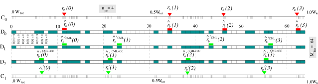
Figure 6: Representation of the HC cell workloads using continuous ($C_{0}$ and $C_{1}$) and discrete ($D_{0}$, $D_{1}$, and $D_{2}$) workload bars, as described in the text. This example is for a simulation on $n_{\rm pr}=4$ processes, with HC-mesh of size $n_{h}^{0}=n_{h}^{1}=n_{h}^{2}=100$ and $N_{\rm bin}=16$. $C_{0}$ and $C_{1}$ are the continuous total workload bars before and after repartitioning, respectively. The filled triangles give the locations of the initial ($C_{0}$) and target ($C_{1}$) partitions. A bin $B(k)$ along the bar $D_{0}$ is filled if and only if the number of dashes in the same interval of bar $C_{0}$ is non-zero. The discrete partitioning states are marked by the filled rectangles above the filled bins of bars $D_{0}$–$D_{2}$. The solution in the discrete space marked on bar $D_{2}$ is obtained by first repartitioning $D_{0}\rightarrow D_{1}$ [holding $r_{b}(0)$ fixed] and then shifting $D_{1}\rightarrow D_{2}$. Finally, the continuous target partitioning state $\{\hat{r}^{\prime}_{b},\hat{r}^{\prime}_{n}\}$ marked on bar $C_{1}$ follows from $D_{2}$. Note that the topology of each bar is a circle formed by connecting its ends.

To solve this problem we compress the cell workload data by discretizing it. The total workload bar is divided into $N_{\rm bin}$ segments per process, or $M_{\rm bin}=n_{\rm pr}N_{\rm bin}$ segments in total. The continuous total workload array $u(r)$ is replaced the much smaller array $B(k)$ with $k\in[0,M_{\rm bin})$. Figure 6 illustrates this with the bars $D_{0}$, $D_{1}$, and $D_{2}$. Each array member $B(k)$ is assigned to the subinterval $[k\,\Delta W,(k+1)\Delta W)$ of the total workload bar, where $\Delta W\equiv W_{\rm tot}/M_{\rm bin}$. The value $B(k)$ is defined as the number of cell boundaries (the dashes) within the corresponding subinterval of the total workload bar. The non-zero members $B(k)>0$ correspond to the filled rectangles of bars $D_{0}$–$D_{2}$ in Figure 6.

Suppose we start from the initial partitioning state $\{r_{\rm b},r_{\rm n}\}$ marked by triangles above $C_{0}$ in Figure 6. We define a discrete partitioning state $\{\hat{r}_{b},\hat{r}_{n}\}$ in the discrete workload space by $\hat{r}_{b}^{i}\equiv[u(r_{\rm b}^{i})/\Delta W]$, $0\leq i<n_{\rm pr}$, where the square brackets signify taking the integer part; $\hat{r}_{n}^{i}$ is the spacing between the consecutive $\hat{r}_{b}^{i}$ along the binned bar of length $M_{\rm bin}$. We define the workloads in the discretized problem as $\hat{W}^{\equiv}\hat{r}_{n}^{i}$. Following equation (26), the load imbalance of a discrete partitioning state is defined by

$$\mathcal{\hat{L}}[\hat{r}_{n}]=1-\frac{\langle\hat{r}_{n}\rangle}{\max\hat{r}_{n}}\ .$$ (36)

The residual load imbalance is redefined in the discrete space as [cf. eq. (30)]

$$\mathcal{\hat{L}_{\rm res}}[\hat{r}^{\prime}_{n}]=\min\limits_{\{\hat{r}^{\prime}_{b},\hat{r}^{\prime}_{n}\}:\;B(\hat{r}^{\prime}_{b})>0}\mathcal{\hat{L}}[\hat{r}^{\prime}_{n}]\ .$$ (37)

The problem of load balancing is posed in the discrete space as finding the discrete target partitioning state $\{\hat{r}^{\prime}_{b},\hat{r}^{\prime}_{n}\}$ that will minimize the load imbalance. We discuss how this is done in the next subsection.

Once the discrete target partitioning state $\{\hat{r}^{\prime}_{b},\hat{r}^{\prime}_{n}\}$ is found, the continuous target partitioning state $\{r_{\rm b}^{\prime},r_{\rm n}^{\prime}\}$ is also found by setting $r_{\rm b}^{\prime\,i}=r^{i}$, where $r^{i}$ is the raw HC index of any cell such that $u(r^{i})\in[\,\hat{r}^{\prime\,i}_{b}\Delta W,(\hat{r}^{\prime\,i}_{b}+1)\Delta W]$. There are, in general, many HC indices that will accomplish this. For example, in Figure 6, the final triangles for bar $C_{1}$ may be placed at any dash lying beneath the rectangles above bar $D_{2}$. The choice is arbitrary and this freedom in setting the target partitioning state will result in negligible differences in the residual load imbalance $\leq 2/M_{\rm bin}$. In practice, we set the partition at the first HC cell that lies in the desired interval.

4.3.2 Finding the Target Partitioning State in the Discrete Case

There are two practical approaches to solving the discrete target partitioning state problem of equation (37).

In the cumulative repartitioning approach we keep the zeroth partition fixed while setting the other ones as close as possible to being equally spaced along the discrete workload bar, subject to the constraints $B(\hat{r}^{\prime\,i}_{b})\neq 0$. It is evident that the resulting target partitioning state is a function of only the initial position of the zeroth partition $\hat{r}^{0}_{b}$ and the discrete workload array $B^{k},\ k\in[0,M_{\rm bin})$.

The cumulative approach alone is not satisfactory for optimizing the discrete load imbalance equation (36) when the cell workloads of some of the HC cells far exceed the discretization load $w(j)\gg\Delta W,\;j\in[0,N_{\rm HC})$. Indeed this problem is illustrated in Figure 6. The initial discrete partitioning state is given by $\hat{r}_{b}=\{11,34,46,62\}$ as shown by the rectangles above the workload bar $D_{0}$. Applying the cumulative approach using the above rule, we have $\hat{r^{\prime}}_{b}^{\rm CML}=\{11,23,43,56\}$, and $\hat{r^{\prime}}_{n}^{\rm CML}=\{12,20,13,19\}$, yielding load imbalance $\mathcal{L}^{\rm CML}=1-(16/20)=0.2$, which is relatively poor. (The superscript CML is used for partitions found with cumulative repartitioning.) This approach uses only the position of the zeroth partition and the discrete cumulative workload array. It is insensitive to differences in the adjacent workloads, e.g. $\hat{r}_{n}^{i}$ and $\hat{r}_{n}^{i+1}$.

In the circular cyclic correction repartitioning approach (denoted by superscript CC), we start from a partition $i$ and shift it to the bin $\hat{r}_{b}^{i}=k$ such that it is the closest possible distance to the bin in the middle of the two adjacent partitions, $k=([\hat{r}_{b}^{i-1}+\hat{r}_{b}^{i+1}]/2$. After the correction of the partition $i$ is done, we move on to the next partition $i+1$, applying the same technique but using the already corrected value for the position of partition $i$. We then continue applying the same scheme for all the other partitions in cycles along the circle $i\in[0,n_{\rm pr})$ until the resulting shifts for all partitions $i\in[0,n_{\rm pr})$ become zero. The resulting positions of the partitions will define the target state in the circular cyclic correction repartitioning approach. This approach if used alone is not satisfactory just as for the cumulative partitioning approach above, however the nature of the problem is completely different. If a large variation in workload $\hat{r}_{n}^{i}$ develops across a large range of indices $i$ (e.g. between $i$ and $i+n_{\rm pr}/d$), this variation will not be suppressed by the circular cyclic correction scheme since only the adjacent partitions $\hat{r}_{b}^{i-1}$ and $\hat{r}_{b}^{i+1}$ are used for correction of any given partition $\hat{r}_{b}^{i}$. On the other hand, all the local fluctuations in workload will be suppressed very effectively.

As we see, the cumulative repartitioning approach and the cyclic circular partitioning approaches smooth the large scale and small scale (in terms of the range of indices) workload fluctuations respectively. Applying the two approaches in sequence works well to provide a nearly optimal solution for the discrete workload. In the example of Figure 6, the bar $D_{2}$ shows the result of applying the circular partition correction approach to the output of the cumulative approach (bar $D_{1}$) obtained from the initial discrete partitioning state (bar $D_{0}$). As follows from the bar $D_{2}$ of Figure 6, the resulting target partitioning state is $\hat{r}_{b}^{i}=\{6,21,38,55\}$ and $\hat{r}_{n}^{i}=\{15,17,17,15\}$. The resulting discrete load imbalance is $\mathcal{\hat{L}}=1-(16/17)=0.06$ is 3.4 times smaller than the load imbalance obtained using only the cumulative method. Our experiments show that the combination of the two approaches results in a good approximation to the load-balanced target partitioning state. The residual load imbalance is generally limited not by our ability to find the optimal solution but instead by the CPU time fluctuations due to variations in cache usage.

5 Particle Data Layout and Communication

In a serial code, the array of particle structures (2.3) is static, that is, it remains fixed length with unchanging particle labels. In a parallel code with domain decomposition, particles may move from one process to another. This not only requires interprocessor communication, it also complicates the storage of particle data. This section discusses our solutions to these problems.

5.1 Linked List Structure, Particle Movement, and Sorting

The particle data are stored as a single local particle array of pointer ${\tt[pa,pa\_f)}$ on each process. A slightly larger range ${\tt[pa,pa\_fa)}$ is allocated to avoid reallocation every timestep. In addition to the particle array, we have a linked list that tells which particles lie in each HC cell. For each HC cell there is a pointer (the root) that (if it is non-null) points into the particle array to the first particle in that HC cell. A complete list of particles within a given local HC region $L_{h}^{i}$ is obtained by dereferencing the appropriate linked list root and then following the linked list from one particle to the next, as illustrated in Figure 7. The linked list also has a root hc_avb that points to disabled particles.

There are several challenges associated with this simple linked list method of particle access. First, one must transfer particles between processes. Second, HC cells are themselves exchanged between processes as a result of repartitioning. Third, one must optimize the traversal of the linked lists to optimize code performance. Finally, one must specify which HC cells are associated with a given process. We discuss these issues in the remainder of this section.

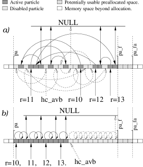
Figure 7: Particle array structure and access in the parallel code. This example corresponds to process $i=0$ of Fig. 5. The HC cells associated with this process are $r=(10,11,12,13)$. The particle arrays are the horizontal bars (with disabled particles corresponding to gaps in the array opened up when particles moved to other processes). The linked list is given by the arrows going from one particle to another; the solid (dashed) arrows give the linked list for the active (disabled) particles. The linked list roots are the pointers hc_avb (for disabled particles) and $r=(10,11,12,13)$ (for active particles) beneath the particle array bars. Each linked list begins at a root and ends with the NULL pointer. The particle array is allocated slightly more storage (pa_fa) than needed (pa_fa). a) The particle array and linked list before sorting. b) The same particles and the linked list after sorting.

During each position advancement equation (11), twice every timestep some particles move across the boundary of their local particle domain. As a result, such a particle is sent from a process $i$ to another process $j$ whose local region $L_{h}^{j}$ it entered. Particles may cross the boundary of any pair of domains. The associated communication cost scales linearly with the $L_{h}$ surface area. The Hilbert curve domain decomposition minimizes this cost because of the low surface to volume ratio (§ 3.2).

When a particle ${\tt p}$ moves outside the local region $L_{h}^{i}$, it leaves a gap in the local particle array. We set the particle mass to $-1$ and call this particle array member a disabled particle. All the disabled particles on each process form a separate linked list with root hc_avb. The particles entering $L_{h}^{i}$ from other processes replace the disabled particles or are added to the end of the particle array.

As a particle initially in process $i$ crosses a boundary to another process, the id of the target process $j$ should be immediately found in order to send this particle to the new process. Dividing the new particle coordinates by the HC mesh spacing gives the new Hilbert curve mesh cell coordinates ${\bf c}$. The target process id can then be found calling Moore’s function for the new HC index $h=\mathcal{H}({\bf c})$. By using the current Hilbert curve partitioning, one finds the id of the target process $j$ from $h$. Once all particles to move have been identified, the particles are transferred between processes.

As we show in Appendix B, Moore’s function calls are relatively expensive. To avoid having this cost each time a particle crosses the boundary, we allocate an extra one layer of HC cells surrounding the boundary of $L_{h}^{i}$, as shown in Figure 8, and we mark the surrounding cells with the ids of the appropriate processes $j$ by calling Moore’s function for each of them exactly once. By doing this once, we avoid calling Moore’s functions in the future. However we still have to call the function for the very small fraction of the boundary-crossing particles that went further than one boundary layer cell in one timestep. The extra layer of HC cells surrounding the local region is also used with the particle-particle force computation as described in §6.3.

We maintain the particle linked list throughout the simulation instead of reforming it each timestep. As particles cross from one HC cell to another — even if they are in the same local region $L_{h}^{i}$ — the linked list is updated to reflect these changes. The particle array is reallocated whenever the fraction of disabled particles exceeds a few percent (the exact value is a parameter set by the user), or the amount of particles exceeds the boundary of the pre-allocated particle array ${\tt pa\_fa}$.

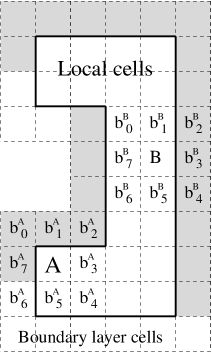
Figure 8: Hilbert curve mesh cells. The cells within the solid line are the $L_{h}^{i}$ cells containing all the particles assigned to process $i$. Information about the layer of boundary cells (all gray and white cells outside the local region) is also stored by process $i$. This information is used both when particles are transferred between processes and during the short-range (particle-particle) force computation. In the latter case, the particle data for the shaded cells is used to compute forces on particles in cells A and B as discussed in § 6.3.

In addition to the pointer to the root of the linked list that contains all the particles within each HC cell, each cell of the local region contains other structure members: the process number the cell belongs to, the current and previous timestep cell workloads required by equation (28), the number of particles in this cell, etc. We will refer to this structure as the HC cell structure and the array of structures for all HC cells the HC cell array. One member of this array has size 16 bytes. When repartitioning occurs, we send and receive the relevant HC cell array members and the particles they contain to the appropriate processes.

Some program components, such as particle position advancement, require access to the complete particle list on each process. All local particles can be accessed using the particle array and filtering out the passive particle array members as follows:

$$\begin{array}[]{l}\tt for(p={\tt pa};\;p<{\tt pa\_f};\;p++)\{\\ \tt\quad if(p{->\hskip 1.42262pt}mass==-1.)\;continue;\\ \tt\quad\ldots\\ \tt\}\ .\end{array}$$ (38)

We found that because of cache memory efficiencies, it is up to ten times faster to use a simple array to access every local particle than it is to dereference the three-dimensional linked list roots for each of the local cells of $L_{h}^{i}$. The reason for such difference is that simple array members are sequential in the machine memory, while the successive linked list members are not, and the CPU cache memory is more effectively used when data are accessed sequentially in an array. The improvement in efficiency is especially important in the particle-particle calculation because each particle is accessed many times during one force computation.

Here we introduce a fast sorting technique that places the particle data belonging to the same HC cell sequentially within the segments of the particle array, ordered by increasing HC-cell raw index. This sorting procedure is performed each timestep before the force computation.

Every timestep, before a force calculation, we follow all the $L_{h}$ cells in the order of their raw HC index, and concatenate their linked lists, resulting in just one linked list of all the particles in the local particle array. Then, using the unnecessary acceleration g0 and g1 members of the particle structure as pointers, we form an extended linked list replacing the old one. The result is a new linked list which can be traversed both forward (using g1) and backward (using g0). Then, starting from the first particle of a simple array of particles, we swap it with the first particle in the extended linked list while the forward and backward pointers of the immediately adjacent within the extended linked list particles being updated. We then proceed to the next particle in the simple array and in the linked list doing the same, until we have sorted the entire particle list. The result of this sorting is illustrated by Figure 7b.

In addition to optimizing the CPU cache memory usage, the above sorting technique eliminates the need to allocate an additional buffer for sending and receiving particles while repartitioning, because all the particles to be moved as the result of repartitioning will occupy contiguous segments in the simple particle array. When the sorting is completed the original linked list is unnecessary and is deallocated in order to be formed again directly using the sorted particle array, before the particle advancement and repartitioning take place.

To transfer particles between processes we use a modification of MPI_Alltoallv that assures no failure will occur if insufficient memory has been pre-allocated for the send and receive buffers. This achieved by using MPI_Alltoall to exchange the numbers of particles to be sent and received and then using as many MPI_Alltoall and MPI_Alltoallv calls as necessary to avoid overflowing the available memory of each processor.

5.2 Scalable Allocation Local Region Access

As mentioned above, during particle exchange and force computation one needs frequent access to a cell’s particle list and other cell data, given the indices ${\bf c}$ of the cell in the HC mesh. The most obvious method is to call Moore’s function $h=\mathcal{H}({\bf c})$ to get the global HC index and then use our table of HC entries (§ 3.3) to convert $h$ into the raw index $r$. The raw index then gives the root to the particle linked list as shown in Figure 7. This method is unsatisfactory because of the expense of calling Moore’s function many times during the force evaluation.

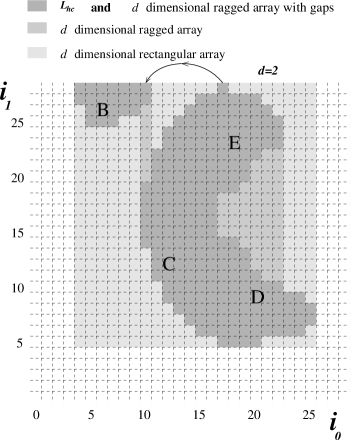
Figure 9: Schematic illustration of the HC local region $L_{h}$ (dark gray) assigned to one process and the rectangular array that includes it (light gray combined with dark gray). The ragged array (middle gray combined with dark gray) requires much less storage but only the ragged array with gaps (dark gray) corresponds exactly to $L_{h}$. Four cells belonging to $L_{h}$ are randomly selected and labelled B, C, D and E.

Another simple method of allocation for the $L_{h}$ cells would be a $d$-dimensional rectangular array of cells holding the frequently used roots of the linked lists to the particles contained in this cell and the total number of particles within it. The access to a HC cell given its coordinates ${\bf c}$ in this case is given by dereferencing the array $r=A[c_{0}][c_{1}][c_{2}]$ in the case of $d=3$, where $A$ is an array of HC cell raw indices (or pointers to HC cells) updated after each repartitioning. The problem here, illustrated in Figure 9, is that many of the entries of $A$ are wasted because the HC local regions are not rectangular parallelpipeds. This can be improved by adjusting the bounds of the array indices $(c_{0},c_{1},c_{2})$ to the extremal values for cells in the local region. The result is a simple $d$-dimensional ragged array, also illustrated in Figure 9.

The optimal method of local region HC cell allocation and access is to add one more dimension to the array of HC cell pointers $A$ used in a simple ragged array. The extra dimension accounts for variable number of disjoint parts in the last dimension. This method allocates the minimal storage needed beyond the number of HC cells in $L_{h}^{i}$. We call this a d-dimensional ragged array with gaps. The HC cell is then obtained by dereferencing the $(d+1)$-dimensional array $A$.

To access a cell with coordinates $c_{0}\ldots c_{d-1}$ using a $d$-dimensional ragged array with gaps, we use $r=A[\,c_{0}][\,c_{1}]\ldots[c_{d-2}][\mathcal{M}][\,c_{d-1}]$, where $\mathcal{M}=\mathcal{M}(c_{0}\ldots c_{d-1})$ is the integer function equal to the number of the completed contiguous intervals in the $c_{d-1}$- ordered set of all the HC cells in the local region having coordinates $c_{0}\ldots c_{d-2}$ and having $(d-1)$-th coordinate less than $c_{d-1}$. For example, in the case $d=2$ of Figure 9, access to the cells B, C, D, and E is given by $r_{B}=A[6][0][26]$, $r_{C}=A[12][0][12]$, $r_{D}=A[20][0][9]$ and $r_{E}=A[18][1][23]$. The disadvantages of the other methods considered above do not apply now: the $(d+1)$-array dereference call is exponentially faster than the function call, and the space allocated exactly equals the required number of $L_{h}$ cells. For $d=3$, the function evaluation $\mathcal{M}(c_{0},c_{1},c_{2})$ takes a time that grows only logarithmically with the number of disjoint parts along the last dimension for a give $c_{0}$ and $c_{1}$.

6 Force Calculation

In this section, we present an efficient method for parallel PM and PP computation of forces for particles within the HC local regions. By using the techniques developed in §§4 and 5, we have made our algorithms load balanced and efficient.

6.1 PM Force Calculation

The PM force calculation requires communication between two different data structures with completely different distributions across the processes. The particles on one process are organized into irregularly-shaped HC local regions. The density and force meshes, on the other hand, have a one-dimensional slab decomposition based on FFTW. The parallel computation is an SPMD implementation of the five PM steps presented in §2.5.

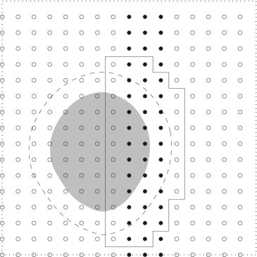
Figure 10: Schematic representation of the sets used in the PM force calculation. The volume within the dotted line is the total simulation volume $V_{0}$, the small circles are the discrete set of PM density gridpoints $G_{0}$. The filled circles are the PM gridpoints within a FFTW slab $j$, $G_{\rm sl}^{j}$. The gray filled region is the HC local region $L_{h}^{i}$. The set of all circles within the dashed line is $\mathcal{G}(L_{h}^{i})$; the set of filled circles within the dashed line is $G_{\rm sl}^{j}\cap\mathcal{G}(L_{h}^{i})$. Extending this last set slightly gives the continuous set within the solid line, $\mathcal{L}(G_{\rm sl}^{j}\cap\mathcal{G}(L_{h}^{i}))$. Eq. (41) gives the intersection of this last set with the gray region$L_{h}^{i}$.

6.1.1 Definitions

We define a few concepts that will be needed in order to describe and implement the data exchange between the two different data structures during the parallel PM force calculation. The various sets used in the calculation are illustrated in Figure 10.

The FFTW parallel Fast Fourier Transform implementation (Frigo & Johnson, 2003) allows one to compute forward and inverse Fourier transforms of the complete three dimensional array of $n_{0}n_{1}n_{2}$ mesh points distributed among the processes $j$ in the form of slabs of ${\tt nloc}(j)\,n_{1}n_{2}$ grid points, where $\sum_{j}{\tt nloc}(j)=n_{0}$, each slab starting at the position ${\tt sloc}(j)=\sum_{i=0}^{j-1}{\tt nloc}(i)$ along the 0-th dimension. We will call these slabs the density or force mesh slabs (depending on the context) and denote them by $G_{\rm sl}^{j}$. The geometry of the slab $G_{\rm sl}^{j}$ is calculated once and for all at the start of the run by calling the FFTW Fourier transform plan initialization routine.

Let us denote the complete discrete set of all density mesh gridpoints needed for a complete Fourier transform by ${G_{0}}$, and the complete continuous set of all positions within the whole simulation volume by ${V_{0}}$. We have

$$\begin{array}[]{ll}G_{\rm sl}^{j}\in{G_{0}},&\bigcup\limits_{j}G_{\rm sl}^{j}={G_{0}}\\ L_{h}^{i}\in{V_{0}},&\bigcup\limits_{i}L_{h}^{i}={V_{0}}\ .\\ \end{array}$$ (39)

Here, $i$ labels the process holding the HC local region while $j$ labels the process holding a given density/force mesh slab.

For a continuous set of positions $L\in{V_{0}}$, let us define $\mathcal{G}(L)$ to be the minimal complete subset of the density grid points ${\bf X}_{\rm gr}\in{G_{0}}$ such that equation (13) is satisfied for any position vector ${\bf X}\in L$. By this definition, if all the local particles are contained within $L$, after the density assignment of Step 1 of the PM force calculation, the only non-zero PM-density grid points of ${G_{0}}$ are in fact within a subset $\mathcal{G}(L)\in{G_{0}}$.

For a discrete subset $G\in{G_{0}}$ of the density gridpoints, let us define $\mathcal{L}(G)$ to be the minimal complete continuous set of points ${\bf X}\in{V_{0}}$ such that equation (13) is satisfied for any ${\bf X}_{\rm gr}\in G$. Now, if all the grid points local to a process are within a subset $G\in{G_{0}}$ of all the particles in the simulation volume ${V_{0}}$, only the particles of the subset $\mathcal{L}(G)$ may acquire any non-zero force contribution from those gridpoints during Step 5 of the PM-force calculation.

6.1.2 Optimal PM Communication Strategy

As we discussed in §2.5, Step 1 of the PM force calculation involves filling the density grid points in $G_{\rm sl}^{j}\in{G_{0}}$ using the particles distributed in the volumes $L_{h}^{i}\in{V_{0}}$. Steps 2–4 involve working only with $G_{\rm sl}^{j}$ and are straightforward since they do not require any interprocessor communication aside from the parallel FFT. During Step 5 the information flows in the exactly opposite direction, therefore an algorithm for Step 1 applies to Step 5 as well with the direction of the information flow reversed. The problem remaining now is for Step 1 of the PM force calculation to decide how to fill the local density grids $G_{\rm sl}^{j}$ from the particles distributed within the local regions $L_{h}^{i}$. To solve this problem we considered a number of approaches described briefly below, but only the last one is implemented in our code and is effective over the entire range of clustering.

a) Sending Particles.

Under this method, each pair $ij$ of processes sends the appropriate portion of the particle data from process $i$ to process $j$ to fill the density mesh $G_{\rm sl}^{j}$ of slab $j$. For each pair of processes the set of the density gridpoints

$$G_{\rm sl}^{j}\cap\mathcal{G}\left(L_{h}^{i}\right)$$ (40)

on process $j$ will be updated with the particles brought from the volume

$$L_{h}^{i}\cap\mathcal{L}\left(G_{\rm sl}^{j}\cap\mathcal{G}\left(L_{h}^{i}\right)\right)$$ (41)

within the HC local region of process $i$.

This method is very efficient for the pairs where the particle sender processes $i$ have low particle number density, thus reducing the number of particles to be sent and the communication cost.

b) Sending Grid Points.

Under this method, each pair $ij$ of the processes fills the portion (40) of the grid points using the local particles within (41), then sends the filled gridpoints to process $j$.

This method performs poorly when the particle number density is low on the sender process, because most of the density values in the message are zero. This method is very efficient for the pairs where the particle sender processes $i$ have a high particle number density: each gridpoint of the sender process contains the contributions from many particles.

c) Combined Particle and Grid Point Send.

Method a) is effective with low particle number density while method b) is effective with high particle number density on the particle sender process. The idea of the combined particle and grid point send method is to choose for each pair of processes the approach that requires sending the least data.

d) Sending Compressed Grid Points.

This approach optimizes the communication cost in both the extreme cases of low and high number density of the particles on the sender process $i$. The idea behind this method is to use the approach b) above and apply sparse compression to the gridpoint messages (40). As we know, the grid point approach performs poorly when the particle number density is low on the sender process. Using sparse compression as we explain in the following subsection significantly alleviates this problem by reducing the message size for the underdense regions $L_{h}^{i}$.

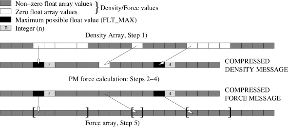
Figure 11: Sparse array compression of density and force messages during PM force computation. The two density arrays (top two bars) are equivalent but the lower one is compressed by run-length encoding. Compression is signalled by a special data value (FLT_MAX) followed by the number of zeros. The compressed array on process $i$ is sent to process $j$ using an MPI function call. A compressed force message is constructed on process $j$ using the template given by the density message. The forces are sent back to process $i$ and expanded. The bracketed values in the bottom array can be ignored because there are no particles nearby the relevant grid points.

6.1.3 Sparse Compression of Grid Point Messages

In a cosmological simulation, the overdense regions have small HC local regions with every grid point having many nearby particles so that the force and density messages are small. On the other hand, low-density regions have large HC local regions with many PM grid points but the density and force messages are made small by the compression method illustrated in Figure 11.

During Step 1 of the PM computation, if a number of binary zeros are encountered in the grid message, they all are substituted by a pair of numbers before sending packets: the first number is a delimiter (an illegal density or force value such as FLT_MAX) and the second number is an integer giving the number of zeros to follow in the original uncompressed message. This technique is called run-length encoding. The resulting compression factor is unlimited and depends on how frequent and contiguous the zero values are positioned in the grid message. The receiver process $j$ simply uncompresses the message by filling the gridpoints within $G_{\rm sl}^{j}\cap\mathcal{G}(L_{h}^{i})$.

During Step 5, the force values are sent from process $j$ to $i$ three times (once for each of the three dimensions). The force array message is identical in the size to the density message that was sent during Step 1 for each pair $ij$ of processes. We compressed the density values in Step 1 using run-length encoding of zero value densities. In the force message the technique runs into a difficulty because the gravitational forces are long range forces by nature and their values are nowhere equal to zero. If we do not compress the force values, there is no advantage in choosing the compressed gridpoint approach, since the force messages would have the same length as the uncompressed density messages.

By using packet information obtained while receiving the density array, we can compress the forces using exactly the same pattern formed by the packets of the density message, as shown in Figure 11. The receiving process will decompress the force and obtain exactly the initial force array excluding the values of force at the array members which were skipped in the density assignment (the square bracketed force values in Fig. 11). This loss of information is however completely irrelevant for interpolation of the force values to the particles in Step 5 because the square bracketed force values in the force array belong to grid points which earlier acquired absolutely no density values from the surrounding particles, which means that for that grid point and for any particle within $L_{h}^{i}$, the gridpoint has no nearby particles [the condition (13) is not satisfied]. Thus the force values at that grid point will not be interpolated to any particles during Step 5.

The idea of sparse array compression is not implemented in the Hydra code (MacFarland et al., 1998). Once implemented it will significantly reduce their communication and memory costs.

6.2 Practical PM Implementation

Equation (40) gives the minimal set of density grid points on process $j$ needing to be filled with values from particles on process $i$. This set is impractical to work with because of its irregular shape. For a practical implementation we embed this region within a rectangular submesh of ${G_{0}}$ during Steps 1 and 5 of the PM force computation, as follows.

For a continuous set of positions inside the simulation volume $L\in{V_{0}}$, let us define $\mathcal{R}(L)$ to be the minimal rectangular subset of density grid points such that $\mathcal{G}(L)\in\mathcal{R}(L)$. For grid points with $\mathcal{R}(L)$ but outside $\mathcal{G}(L)$ we set the density values to zero. It follows at once that if we use

$$G_{\rm sl}^{j}\cap\mathcal{R}\left(L_{h}^{i}\right)$$

instead of equation (40) for the definition of PM grid point messages, we will have the rectangular mesh $\mathcal{R}\left(L_{h}^{i}\right)$ for interpolation of density for particles within $L_{h}^{i}$, and this still give the correct result. However, since the extent of the local region $L_{h}^{i}$ inside the simulation box is not limited, neither is the extent of $\mathcal{R}\left(L_{h}^{i}\right)$. For example, when $L_{h}^{i}$ consists of just two cells with the coordinates $(0,0,0)$ and $(n_{h}^{0}-1,n_{h}^{1}-1,n_{h}^{2}-1)$, it is easy to see from the definition that $\mathcal{R}\left(L_{h}^{i}\right)$ encloses the whole simulation density mesh ${G_{0}}$ as a subset and this is too much memory space for allocation on a process.

To avoid this problem, we dissect the local region $L_{h}^{i}$ uniformly into $n_{k}^{i}$ slices $M^{ik}$ along the 0-th dimension so that the extent of each slice along the 0-th dimension will not exceed $n^{0}/n_{\rm pr}$. Using the previous equation we have, now summed for all the receiving processes $j=0\ldots n_{\rm pr}-1$

$$\sum_{j=0}^{n_{\rm pr}-1}G_{\rm sl}^{j}\cap\mathcal{R}\left(L_{h}^{i}\right)=\sum_{j=0}^{n_{\rm pr}-1}G_{\rm sl}^{j}\cap\mathcal{R}(\,\sum_{k=0}^{n_{k}^{i}-1}M_{h}^{ik}\,)=\sum_{k=0}^{n_{k}^{i}-1}\left(\sum_{j=0}^{n_{\rm pr}-1}G_{\rm sl}^{j}\cap\mathcal{R}(M_{h}^{ik}\,)\right)\ .$$ (42)

For each slice $M_{h}^{ik}$ of the HC local region $L_{h}^{i}$, the density is interpolated onto the rectangular mesh $\mathcal{R}(M_{h}^{ik}\,)$ which is small enough to be allocated since its extent in the 0-th dimension is limited by roughly $n^{0}/n_{\rm pr}$ grid points. Then, the messages under the inner sum of equation (42) are sent to processes $j=0..n_{\rm pr}-1$. The procedure is repeated for each slice $M_{h}^{ik}$.

In the code presented in this paper we use the blocking MPI routines for PM message communication, which requires synchronization between each pair of processes exchanging the message. In order to reduce waiting time, MPI allows bi-directional blocking communication using MPI_SendRecv. In the above equation the process $i$ is described as the sender of the PM-grid messages obtained by interpolation from the particles within $L_{h}^{i}$ to the processes $j$ in order to update their FFTW-slabs $G_{\rm sl}^{j}$. Note however, that the same process $i$ also behaves as a receiver of the PM grid messages from the other processes $j$ in order to update the FFTW-slab $G_{\rm sl}^{i}$. The set of the received messages is obtained by simply swapping the indices $i$ and $j$ in the above equation. Adding the two together we have for the set of gridpoints participating in the communication on process $i$ in both directions

$$\sum_{j=0}^{n_{\rm pr}-1}\left[G_{\rm sl}^{j}\cap\mathcal{R}\left(L_{h}^{i}\right)+G_{\rm sl}^{j}\cap\mathcal{R}\left(L_{h}^{i}\right)\right]=\sum_{k=0}^{n_{k}^{ij}-1}\sum_{j=0}^{n_{\rm pr}-1}\left[\;G_{\rm sl}^{j}\cap\mathcal{R}(M_{h}^{ik}\,)+G_{\rm sl}^{i}\cap\mathcal{R}(M_{h}^{jk}\,)\right]\ ,$$ (43)

where ${n_{k}^{ij}}\equiv\max(n_{k}^{i},n_{k}^{j})$ and the $M_{h}^{ik}$ is defined to be an empty set for $k\geq n_{k}^{i}$ .

In order to access particles in a given slice $M_{h}^{ik}$ of the local region we use the particle access technique described §5.2. The sorting technique described in §5.1 speeds up the density and force interpolation. The timing of the interpolation for each HC cell gives the PM part of the HC-cell workloads in equation (24).

The above procedure is used for both density and force interpolation in the PM force calculation. In the current implementation, the MPI messages are blocking, which means additional waiting time. In a subsequent paper we describe the implementation of non-blocking communication resulting in a significant speedup of the PM calculation.

6.3 PP Force Calculation

The particle-particle (PP) force calculation increments forces acting on each of the particles in a pair if the particles are closer than $\tilde{R}_{\max}$.

The method of particle access developed in §5.2 allows one to access all the particles within a given HC cell. From equation (19), HC cells are coincident with the chaining mesh cells needed for the PP force calculation. To see how the communication and computation work, consider the example of Figure 8. To compute the PP force for a particle ${\tt p}$ within chaining mesh cell $A$, the particle data in the surrounding cells $b^{A}_{0}\ldots b^{A}_{3}$ are required. The particle data within the cell $b^{A}_{3}$ are locally available. However one needs to bring the positions and masses from the other processes to get the particle data for the boundary layer cells $b^{A}_{0}\ldots b^{A}_{2}$. Once the particle data from the boundary layer cells are gathered, the PP force calculation may be performed by pair summation, after which the resulting forces for the particles within $b^{A}_{0}\ldots b^{A}_{2}$ are sent back to their processes where the PP forces of the original particles are incremented.

The same algorithm applies to any other cell within $L_{h}$, for example the cell $B$ of Figure 8, for which the particle data for $b^{B}_{0}$ and $b^{B}_{1}$ are available locally while the particle data for cells $b^{B}_{2}$ and $b^{B}_{3}$ must be brought to the local process from the others. Because of its pairwise nature only half the surrounding cells are needed for the PP force calculation for each HC cell. In total, the particle data for the non-local cells shaded in Figure 8 are required for the PP force calculation for each particle within $L_{h}$. The amount of communication needed for a complete PP force calculation is proportional to the number of particles in the cells required to be brought from the other processes through the boundary layer cells.

If the PP pair summation step is started synchronously on all processes, it will finish at approximately the same time on all processes if the load imbalance is low. Otherwise, the processes that complete the PP force computation first will have to wait for the remaining processes to finish their pair summation. Since the pair summation is the most time-consuming step of P³M, it is crucial that the procedure be load-balanced. This is accomplished using the methods of §4. The CPU time of the pair summation step is used in the cell workload calculation of equation (24). The particle access time in the pair summation loop is minimized by pre-sorting the particles as described in §5.1.

6.4 Memory Management

In early versions of our code, the memory often exceeded the available resources causing the code to crash. By implementing runtime tracking of memory usage we were able to identify the problems and optimize the memory requirements. Memory usage was reduced largely in three ways: the irregular shaped local domain memory technique of §5.2, the elimination of particle buffer allocation while repartitioning, and memory balancing when necessary during repartitioning as described in §4.2.

	Notation	Memory Size, per process $i$	Total Memory size
Particle array	$M_{\rm P}$	$4\,\hbox{bytes}\times 11N(i)$	$4\,\hbox{bytes}\times 11N$
Particle linked list	$M_{\rm L}$	$4\,\hbox{bytes}\times N(i)$	$4\,\hbox{bytes}\times N$
HC mesh	$M_{\rm HC}$	$4\,\hbox{bytes}\times 5r_{\rm n}^{i}$	$4\,\hbox{bytes}\times 5n_{h}^{0}n_{h}^{1}n_{h}^{2}$
Green’s function	$M_{\rm G}$	$4\,\hbox{bytes}\times{\tt nloc}(i)\,n^{1}(n^{2}/2+1)$	$4\,\hbox{bytes}\times n^{0}n^{1}(n^{2}/2+1)$
Density and Force meshes	$M_{\rm PM}$	$4\,\hbox{bytes}\times 2\,{\tt nloc}(i)\,n^{1}(n^{2}+2)$	$4\,\hbox{bytes}\times 2n^{0}n^{1}(n^{2}+2)$
FFTW scratch space	$M_{\rm FFT}$	$4\,\hbox{bytes}\times{\tt nloc}(i)\,n^{1}(n^{2}+2)$	$4\,\hbox{bytes}\times n^{0}n^{1}(n^{2}+2)$
PP boundary layer particles	$M_{\rm PP}$	$4\,\hbox{bytes}\times 8\Delta n_{\rm PP}$	$4\,\hbox{bytes}\times 8\sum\Delta n_{\rm PP}$

Table 3: Dominant memory requirements of the parallel GRACOS code. Here $n(i)$ is the number of particles and ${\tt nloc}(i)$ is the thickness of the PM slab , both on process $i$.

In Table 3 we list the main memory requirements for our GRACOS code. Compared with the memory requirements for the serial code in Table 1, we were able to reduce the size of the particle linked list by 50%. Note that the HC mesh is the parallel equivalent of the serial chaining mesh but requires 5 times more storage. (This is still less than the storage required for the linked list, so we have accomplished a net savings.) The FFTW scratch space is optional but significantly improves FFTW performance, so we allocate it. The maximum memory allocated per process each timestep can be obtained by combining the tabulated values in the sequence that follows their actual allocation and release in the code. For example, the memory spaces $M_{\rm PM}$, $M_{\rm FFT}$ and $M_{\rm PP}$ are allocated when the memory space $M_{\rm L}$ is released. The actual memory usage along with the detailed measurements from a $800^{3}$ run are described in §7.3.

7 Tests

The first and most important test was to verify that our parallel PM and P³M codes give identical results to the serial codes (both the original Fortran codes and their C translations) when given identical inputs, to within the precision of machine roundoff error. The serial codes have been thoroughly tested by Gelb & Bertschinger (1994).

The remaining tests presented in this section test the performance of the parallel codes in order to optimize the performance. Several of the innovations described in the preceding sections were devised in response to performance tests.

The PM test presented in §7.1 was performed on a beowulf cluster consisting of 7 nodes each with a 1.7 GHz Pentiun-4 processor with 256 KB L2 cache memory, 1 GB RAM memory, and 34 GB of hard drive, connected by 100 Mb/s ethernet. The Linux gcc compiler was used. This cluster has a Linpack performance of 15 GFlops.

The rest of the test runs were performed on a beowulf cluster consisting of 20 dual Xeon 2.4 GHz Pentium-4 and 512 KB L2 cache memory processor computing nodes each containing 4 GB RAM memory and 360GB of disk, connected by gigabit Ethernet. The Intel icc compiler was used. This cluster has a Linpack perfomance of 70 GFLops.

7.1 PM Simulation of Extremely Clustered Matter

Cosmological initial conditions for cold dark matter were generated for a simulation with $512^{3}$ particles and grid points, with a power spectrum having a Gaussian cutoff at a wavelength equal to one-fourth of the box size and white noise on larger scales. The resulting nonlinear evolution, shown in Figure 12, leads to the formation of two massive particle clusters displaying many phase space caustics. The initial conditions were evolved using both the llpm-sl and GRACOS codes to compare their timing performance.

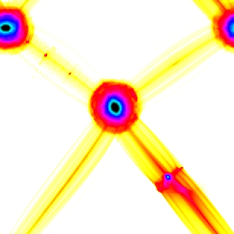
Figure 12: Projected particle distribution for the entire PM simulation volume of $512^{3}$ particles at timestep 5693. False colors scale with the logarithm of projected mass density. Strong clustering like this favors dynamic rather than static domain decomposition methods.

This test used an early version of GRACOS with only PM forces. Since we did not compute PP forces the constraint given by equation (19) was not in effect. Instead we set our HC mesh spacing to $\Delta\tilde{x}_{h}^{i}\geq 1.5$. The sorting technique described in §5.1 was not implemented. Instead of equation (24), we used the number of particles in a cell to define the HC cell workload. Repartitioning therefore resulted in an approximately equal number of particles on all processes at each timestep.

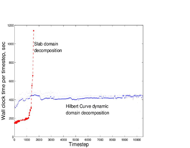
Figure 13: Timing performance comparison of a Hilbert curve dynamic domain decomposition code GRACOS  and a fixed (slab) domain decomposition parallel code llpm-sl for the identical run showed in Fig. 12. The runs start from the linear regime and are evolved using only PM forces.

Figure 13 shows the wall clock time per timestep for the Hilbert curve code GRACOS and the fixed slab domain decomposition code llpm-sl. As we see from the Figure, the HC-based PM code evolves very far into the regime of strong matter clustering without any significant slowdown. On the other hand, the slab decomposition code grinds to a halt because of the growing memory imbalance arising in any fixed domain decomposition method. As more and more particles end up on one process, not only does its CPU workload grow, but the process eventually runs out of memory and starts paging to disk, slowing down the evolution by orders of magnitude. Only a dynamic domain decomposition can handle clustering as extreme as that shown in Figure 12.

Even though the HC code is vastly superior to slab decomposition under strong clustering, it is slower at early times. This is mainly because the local regions are displaced from the FFTW slabs in the GRACOS code, therefore more communication is required. In addition, since the non-blocking communication was not implemented (see § 6.2), there is some unnecessary waiting time in the HC code.

7.2 P³M Simulation of $\Lambda$CDM without Repartitioning

An extensive series of tests were performed using the GRACOS code to assess its behavior under a wide range of clustering conditions. All of the runs use one particle per PM mesh cell in a cube of size $L^{0}=L^{1}=L^{2}=200$ Mpc. The Plummer softening length was set to $\tilde{\epsilon}=0.4$ (i.e. 40% of the PM mesh spacing). We generated the initial conditions for the $\Lambda$CDM model (with $\Omega_{m}=0.27$, $\Omega_{\Lambda}=0.73$, $H_{0}=71$ km s^-1 Mpc^-1, $\sigma_{8}=0.84$, $n=0.93$ from Bennett et al. 2003) using the BBKS transfer function in a C parallel version of grafic1 (Bertschinger, 1995). The timestep parameter of equation (12) was set to $\eta_{t}=0.05$.

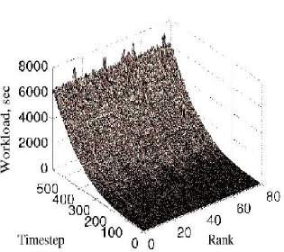
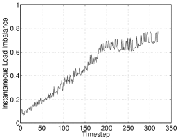
Figure 14: Left: Time required to complete the pair summation step on each process (labelled by MPI rank) as a function of timestep during a $800^{3}$ P³M run without repartitioning. Right: Instantaneous load imbalance as a function of timestep for the same run.

As a first test of the full GRACOS code we ran a simulation with $800^{3}$ particles and grid points with no repartitioning. This run was performed with 80 processes on 20 nodes (40 CPUs using hyperthreading, which treats a physical CPU as two virtual CPUs with improved performance). Without repartitioning the HC local regions on each process remain the same throughout the run. The results appearing in Figure 14 are predictable. A few processes require much longer time to finish the pair summation, leading to a large load imbalance. Late in the simulation, only about $1-\mathcal{L}=25\%$ of the net wall clock time is spent doing computation; most of processes sit idle most of the time waiting for the heavily loaded processes to finish the PP pair summation.

7.3 P³M Simulation of $\Lambda$CDM with Repartitioning: Load Balancing

We reran the $800^{3}$ simulation of §7.2 on 80 processes with repartitioning enabled in order to load balance the computation. Because of the strong increase in clustering and the resulting growth of the PP pair summation time, the wall clock time to complete one timestep increased from just over 4 minutes at the beginning of the simulation to 2 hours at the end (timestep 569, when the expansion factor was $a=0.7$, or a redshift of $z=0.43$). The simulation, finished on August 29 2004, took two weeks to get to this point and would have required another month to evolve to $a=1$ provided it remained well load balanced. In a subsequent paper we introduce an adaptive technique that substantially decreases the PP workload enabling longer and more highly clustered simulations to be performed in much less time. A projection of the particle distribution at timestep 566 for this simulation was used in Figures 3 and 4. At the end of the simulation the Layzer-Irvine energy conservation check (eq. 9) was satisfied to a precision $\tilde{E}_{\rm con}/\tilde{E}_{g}=5\times 10^{-5}$. (Energy conservation can be as much as 100 times worse when clustering is very weak and the PM force contributions dominate over PP.)

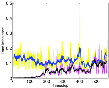
Figure 15: Instantaneous (blue and yellow curves) and residual (black and pink curves) load imbalance as a function of timestep for the $800^{3}$ P³M run with Hilbert curve repartitioning on 80 processes. The yellow and pink curves give the load imbalance of every timestep; the blue and black curves apply boxcar averaging over 10 timesteps to reduce the fluctuations. The residual load imbalance is the minimum possible load imbalance that could be achieved by repartitioning in the absence of fluctuations.

In Figure 15, we present the instantaneous and residual load imbalance as functions of timestep. The effective load imbalance (not shown) is almost identical to the instantaneous load imbalance but is lower by 10% for the highest spike at timestep 403. The differences between these various measures of load imbalance are explained in §4.1.

One of the main results of this paper is that the time-averaged instantaneous load imbalance generally remains between 10 and 15% (averaging 12%) and does not grow steadily worse with time. By contrast, without Hilbert curve dynamic domain decomposition, by timestep 300 the load imbalance exceeded 70% (Fig. 14).

At early times the residual load imbalance is much less than the instantaneous load imbalance because fluctuations in cache usage limit our ability to predict the optimal repartitioning for the next timestep. Later in the run, the residual load imbalance grows when a small number of highly-occupied HC cells begin to dominate the CPU time in the PP force calculation, as we discuss further below.

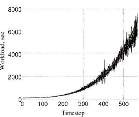
Figure 16: Instantaneous workload of each process as a function of timestep. Left: view from an oblique angle. Right: projected view down the rank (process number) axis.

To analyze the limitations of our load balancing algorithm, in Figure 16 we plot the instantaneous workload measured every timestep for every process using equations (24), (25), and (28). The workload is approximately the CPU time required for PP pair summation summed over all the local HC cells on each process. The main pattern seen is the steady rise of the average PP workload with timestep due to the increase in clustering caused by gravity. After that, one sees in the left plot four spikes in processes 14, 34, 54, and 74. Given our assignment of processes to nodes, these processes reside on the same physical node 14 and are probably caused by competition of these processes for memory access. Fluctuations in cache memory usage are probably also responsible for the smaller fluctuations in workload superposed on the steady rise with timestep in the right plot.

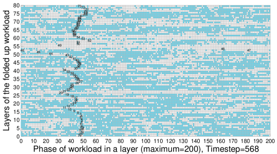
Figure 17: The discrete workload array for timestep 568 of the same simulation analyzed in Figs. 15 and 16. The discrete workload array is a one-dimensional array of $M_{\rm bin}=1600$ cells folded into a set of 80 layers (along the vertical axis) of length 200 (along the horizontal axis). Blue cells contain at least one boundary between HC cells; a continuous white segment represents a single HC cell. The target discrete partitions $\hat{r^{\prime}}_{b}^{i}$ are marked with process rank $i$ (cf.  bar $D_{2}$ in Fig. 6).

To investigate further the cause of growing residual load imbalance, in Figure 17 we present the discrete workload array (§ 4.3) at timestep 568. A perfectly load-balanced partitioning state would correspond to a target partitioning state with all boundaries lined up in one vertical column. (In that way, a fraction $1/80$ of the work would be assigned to each of the 80 processes.) However, this is impossible because processor boundaries cannot occur in white sections (where by definition there are no processor boundaries) and every column contains some white space. Instead, the (nearly) optimal solution is found using the method described in §4.3.2 and used to define the target partitioning state corresponding to the black numbers giving the process boundary for each process.

Figure 17 shows that the workloads of processes 48–53 are hard to adjust by repartitioning since most of the cells of the workload array in their vicinity are white. This occurs because these processes have a small number of HC cells in very high density regions requiring a significant amount of CPU time to complete their PP force calculations. The resulting uneven workload assignment causes the systematic increase in the measured instantaneous workloads for these processes after timestep 470 in Figure 16 and therefore an increase in the residual load imbalance in Figure 15. We would not be able to carry out the P³M calculation much further before a single HC cell begins to take more time than the local regions of other processes, leading to severe load imbalance (eq. 31). Even with the strong variation in workload present after timestep 500, Figure 15 shows that our algorithm manages to achieve an instantaneous load imbalance almost as small as the optimal (residual) imbalance. We expect even better performance when (in a later paper) adaptive mesh refinement is used to alleviate the PP pair summation workload.

7.4 P³M Simulation of $\Lambda$CDM with Repartitioning: Local Regions, Timing, and Memory Usage

We continue discussing the same long $800^{3}$ P³M simulation as in the preceding section but now focus on aspects of code performance other than load balance.

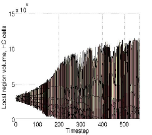
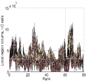
Figure 18: Volume of HC local regions, as a function of timestep and process rank. In the left panel, the full range of process ranks is shown for each timestep. In the right panel, the full range of timesteps is shown for each process rank. The average volume of local regions is $3\times 10^{5}$ cells.

In Figure 18 we plot the volume $r_{\rm n}^{i}$ of HC local regions as a function of timestep and process number. The local region volume is large when the workload per HC cell is small (i.e., in low-density regions) and is small when the workload is high (i.e., in dense particle clusters). At the beginning of the simulation, all $287^{3}$ HC cells are uniformly divided between the processes. As clustering grows, a huge range of volumes develops as the local regions adjust to follow the change in their workload. Because of the compactness property of the Hilbert curve, particle clusters or voids tend to occupy adjacent processes.

At timestep 568 (the end of the run), the smallest local regions belong to processes $i=20$, 34, 48, 49 and 54, with $r_{\rm n}^{i}=7$, 282, 4, 29, and 4 cells, respectively (see also their workload structure in Fig. 17). Because the run is well load balanced, the small number of local cells per process implies that the workloads of those cells greatly exceed the average. Indeed, the average value of workload per cell in the whole simulation box is $W_{\rm tot}/(n_{h}^{0}n_{h}^{1}n_{h}^{2})=4.23\times 10^{-8}\,W_{\rm tot}$. A process with only $4$ local cells has (on average) workload $W_{\rm tot}/(4n_{\rm pr})=3\times 10^{-3}W_{\rm tot}$, which is five orders of magnitude higher than the average workload of a cell in the simulation volume. Such a high cell workload results from the huge local number density of particles for these cells leading to a heavy PP-force calculation load (eq. 24). Indeed, process 48 holds $1.9\times 10^{5}$ particles or $8.8\times 10^{3}$ times the average. Also, by an unfortunate coincidence, two of the five most heavily loaded processes (34 and 54) ended up on the same compute node, leading to heavy demands on memory and (apparently) causing the spikes seen in Figure 16.

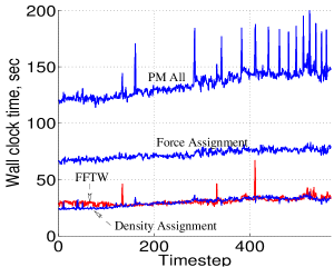
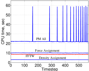
Figure 19: Structure of the wall clock time (left) and CPU time (right) of the PM force computation. The times are averaged over processes. The 40-second spikes are due to recomputation of the PM Green’s function when the code is restarted every 24 hours. Unlike the wall clock time, the CPU time does not increase because it does not include time spent waiting for processes to finish.

Next we present a detailed analysis of the timing structure of the force calculation.

In Figure 19 we present the structure of the wall clock and CPU time of the PM force computation. We see that the wall clock time on average exceeds the CPU time by a factor of 7 during the run, which means that during the PM force calculation processes spend 85% of their time waiting for interprocessor communication requests to clear. This is a big fraction that can be reduced significantly by the use of non-blocking requests for PM density and force grid sends and receives between the local HC and FFTW slabs (see § 6.1). However, except at the early stages of clustering (the initial timestep was 4 minutes, growing to 2 hours), the PM time is a small fraction of the total timestep.

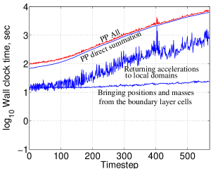
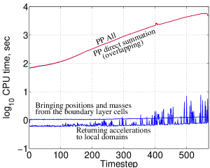
Figure 20: Structure of the wall clock time (left) and CPU time (right) of the PP force computation. The times are averaged over processes.

In Figure 20 we present the wall clock and CPU timing for the parallel PP force computation. Three tasks are required for a PP step (§ 6.3). First, particle positions and masses must be brought from boundary layer cells on other processes. Second, pairwise gravitational accelerations are computed by direct summation. Finally, accelerations are returned across the domain boundaries as needed. The cost of pair summation dominates the other tasks and has essentially equal wall clock and CPU times (hence involves almost no waiting). For the communication tasks (sending and receiving particle positions, masses, and accelerations) the wall clock time greatly exceeds CPU time because of blocking communication and the resulting waiting time.

Figure 20 shows that the waiting time during PP is dominated by the return of accelerations after their computation. The wall clock time of this task is about 10% that of the pairwise computation. This is because the load imbalance in the code arises almost entirely during the pairwise force computation. Figure 15 shows that the average instantaneous load imbalance is approximately 12% during the whole run. From equation (26), we see this means that one of the processes requires about 12% more time to complete its pair summation than the others (since the total CPU time is dominated by pair summation). Other processes cannot get all their accelerations returned until this process finishes computing them, which explains the order of magnitude difference in the direct summation and return of acceleration wall clock times.

The P³M force calculation accounts for nearly all the time of each timestep. Some time is spent by repartitioning every timestep. Because repartitioning may result in the exchange of many HC cells and particles between processes, we might expect it to take a significant amount of time. In fact, the total wall clock time spent on load balancing (analyzing workloads, finding the target partitioning state, and exchanging data between processes) takes on average less than 20 seconds per timestep, or less than the CPU time of the PM force calculation. Occasionally the repartitioning time spikes up to nearly 80 seconds but it does not grow steadily with clustering. The load balancing time is generally less than 8% of the total wall clock time per timestep. Less than one percent of the wall clock time is spent updating particle positions and velocities and exchanging the particles between processes as a result of their motion.

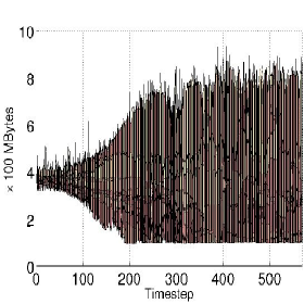
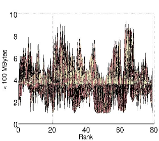
Figure 21: Maximum total memory allocated by any node, as a function of timestep (left panel) and process rank (right panel).

Next we analyze memory usage during the run. In §6.4 we estimated the memory requirements. We now compare these estimates with measured memory usage.

In Figure 21 we present the maximum amount of total memory allocated by a given process during any timestep within the run. In Linux, a memory request in excess of about 1.4 GB on any process will crash the run (see § 2.7). As expected, at the beginning of the run when particles are nearly uniformly distributed, each process requires approximately the same amount of memory. Using the data from Table 3, we estimate the initial maximum memory usage to be $M_{\rm P}+M_{\rm HC}+M_{\rm G}+M_{\rm PM}+M_{\rm FFT}=(11+0.23+0.5+2+1)\times 800^{3}/n_{\rm pr}\times 4\,\hbox{bytes}=359.6$ MB, compared with the measured value of 366.5 MB. Most of the difference comes from the table of HC entries (3.4 MB) plus slight variations in the HC mesh and particle storage among processes.

At the end of the run the domains of each process have changed substantially. All processes require at least $M_{\rm G}+M_{\rm PM}+M_{\rm FFT}=(0.5+2+1)\times n^{0}n^{1}n^{2}\times 4/n_{\rm pr}=85.4$ MB, compared with the measured minimum value of 98.3 MB. The maximum amount of memory varies substantially and is hard to control at the final timesteps. We limit the maximum memory using the techniques mentioned in §6.4. During the last timestep 569, the maximum memory usage was reached on process 27. During this timestep process 27 changed the volume of its domain from $1.23\times 10^{6}$ HC cells to $0.94\times 10^{6}$ cells, which reduced the number of particles in its local region from $17.7\times 10^{6}$ to $14.2\times 10^{6}$. The number of PP boundary layer particles received by this process (see § 6.3) during the same timestep was $1.1\times 10^{6}$. The measurement of 857.8 MB compares with the predicted value (before repartitioning) $M_{\rm P}+M_{\rm HC}+M_{\rm G}+M_{\rm PM}+M_{\rm FFT}=(778.5+24.6+12.8+51.2+25.6)\times 10^{6}=851.3$ MB. Again the table of HC entries (3.4 MB) makes up most of the difference.

The reader will notice the similarity between Figures 18 and 21. The maximum memory usage tracks the volume of HC local regions because the most variable memory element is the number of particles, which correlates strongly with the number of HC cells. Strikingly, the CPU time for the PP pair summation does not correlate well with the number of particles or the maximum memory usage. At the last timestep, process 27 (which used 857.7 MB) took 6037 seconds of CPU time for the pair summation while process 48 (which used 98.1 MB) took 7152 seconds. This is a measure of the success of load balancing, which attempts to equalize CPU time rather than memory usage across all processes.

7.5 Parallel Scalability

A key test of any parallel code is its scalability as the problem size and/or number of CPUs increase. For a fixed problem size, if the wall clock time scales inversely with the number of CPUs, then one may use more CPUs to realize the proverb “many hands make light work.” The ideal inverse scaling is readily achievable with so-called “embarrassingly parallel” codes that require little or no communication, but high efficiency is much more difficult to achieve for algorithms as complex as P³M. Even if a code does not scale perfectly with a fixed problem size, it may scale well when the problem size is increased, enabling one to make effective use of supercomputers with hundreds or thousands of processes to perform very large simulations.

Run	$N_{\rm gr}$	Nodes	Proc./node	$n_{\rm pr}$	(Wall Clock Time)$\times$Nodes
3a	$288^{3}$	1	4	4	79.2h
3b	$288^{3}$	2	4	8	82.8h
3c	$288^{3}$	3	4	12	87.0h
3d	$288^{3}$	4	4	16	91.4h
3e	$288^{3}$	8	4	32	108.1h
3f	$288^{3}$	10	4	40	104.9h
3g	$288^{3}$	12	4	48	111.8h
3h	$288^{3}$	16	4	64	126.0h
3i	$288^{3}$	20	4	80	152.3h
4a	$288^{3}$	10	2	20	148.6h
4b	$288^{3}$	20	2	40	170.2h
5a	$384^{3}$	5	4	20	421.2h
5b	$384^{3}$	10	4	40	470.7h
5c	$384^{3}$	14	4	56	503.5h
5d	$384^{3}$	20	4	80	589.1h

Table 4: Scalability Runs.

We tested the scalability of GRACOS using two problem sizes ($288^{3}$ and $384^{3}$ $\Lambda$CDM in a 200 Mpc box with Plummer softening length $\epsilon=0.1$ Mpc, evolved to redshift zero, taking 634 and 657 timesteps, respectively) and a range of numbers of computing nodes as shown in Table 4. Each computing node has two CPUs. The runs have either two processes per node (one per CPU, Runs 4a,b) or four processes per node (two per CPU, using Intel hyperthreading). For perfect scalability, the times in the last column would be equal for simulations of the same grid size $N_{\rm gr}$.

From Table 4 we may draw several conclusions. First, GRACOS does not scale perfectly like an embarrassingly parallel application. On the other hand, increasing the number of processes up to 80 leads to a steadily decreasing wall clock time. Comparing Runs 3a and 3g, we see that for up to 48 processes, the wall clock time scales as $n_{\rm pr}^{-0.86}$. Hyperthreading also gives a significant speedup. Comparing Runs 3f and 4b, which have the same total number of processes but different numbers of compute nodes, we see that hyperthreading improves the code performance by a factor 1.62. We also see that the code scales reasonably well as the problem size is increased. Comparing Runs 3f and 5b, the wall clock time is proportional to $N^{1.74}$ where $N$ is the number of particles. When the wall clock time is dominated by PP pair summation, we expect scaling as $N^{2}$.

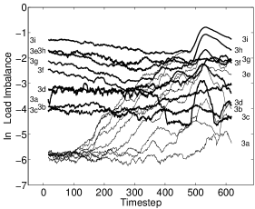
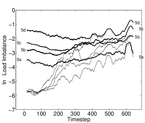
Figure 22: Instantaneous (heavy lines) and residual (thin lines) load imbalance as a function of timestep for Runs 3 ($N_{\rm gr}=288^{3}$, left) and 5 ($N_{\rm gr}=384^{3}$, right). The individual runs are labelled.

The most significant deviations from perfect scalability arise with the largest numbers of processes, in particular Runs 3h, 3i, and 5d. These arise from load imbalance, as shown in Figure 22. A significant increase in load imbalance shows up after timestep 500 in Runs 3 and timestep 600 in Runs 4 due to the formation of a dense dark matter clump. When the number of processes is sufficiently large, this leads to one or a few HC cells beginning to take as much time for PP pairwise summation as the average time for the other processes. According to equation (31), the result is a growing residual load imbalance. Scalability breaks down beyond a certain number of processes, given by equation (32). Once the performance saturates, the instantaneous and residual load imbalance match because it is no longer possible to improve the load balancing by rearrangement of the partitioning.

Although the performance of GRACOS is limited by the PP pair summation and not by the PM force computation, it is worth recalling that, because the current code uses blocking sends and receives to pass data between the particle and grid structures, the PM time also scales imperfectly. When we implement adaptive P³M, the PP time will decrease significantly so that the PM time becomes a significant fraction of the total wall clock time. To improve the parallel scaling, it will be important to implement non-blocking communication for the PM particle/grid messages.

8 Conclusions

Parallelizing a gravitational N-body code involves considerably more work than simply computing different sections of an array on different processors. The extreme clustering that develops as a result of gravitational instability creates significant challenges. A successful parallelization strategy requires careful consideration of CPU load balancing, memory management, communication cost, and scalability.

The first decision that must be made in parallelizing any algorithm is how to divide up the problem to run on multiple processes. In the present context this means choosing a method of domain decomposition. Because P³M is a hybrid algorithm combining elements of three-dimensional rectangular meshes and one-dimensional particle lists, we chose a hybrid method of domain decomposition. A regular mesh, distributed among the processes by a simple slab domain decomposition, is used to obtain the PM force from the mesh density. A one-dimensional structure — the Hilbert curve – is introduced to handle the distribution of particles across the processes and to load balance the work done on particles.

Implementing Hilbert curve domain decomposition in a particle code is the major innovation of our work. To take full advantage of it we had to employ a number of advanced techniques. First, in §4 we devised a discrete algorithm to find the nearly optimal partitioning of the Hilbert curve so as to achieve load balance, the desirable state in which all processors have the same amount of work to do. This is a much greater challenge in a hybrid code than in a purely mesh-based code such as a hydrodynamic solver or a gridless particle code such as the tree code. We then made the domain decomposition dynamic by repartitioning the Hilbert curve every timestep, allowing us to dynamically maintain approximate load balance even when the particle clustering became strong.

In §5.2 we presented a fast method for finding the position of a cell along the Hilbert curve given its three-dimensional location. This procedure allows us to access arbitrary cells in a general irregular domain by a lookup table much faster than using the special-purpose Hilbert curve function of Moore (1994).

In §6.1.3 we introduced run-length encoding to greatly reduce the communication cost for transferring information between the particle and mesh structures required during the PM force computation.

In §5.1 we optimized the particle distribution within each process so as to improve the cache performance critical for efficient pair summation in the PP force calculation.

By choosing the domain decomposition method appropriate for each data structure, and by implementing these additional innovations, we achieved good load balance and scalability even under extreme clustering. The techniques we introduced for effective parallelization should be applicable to a broad range of other computational problems in astrophysics including smooth-particle hydrodynamics and radiative transfer.

Tests of our algorithm in §7 showed that we achieved our goals of scalability and load balance, with two caveats mentioned at the end.

In Figure 13 we demonstrated the importance of using a dynamic three-dimensional domain decomposition method instead of a static one-dimensional slab decomposition. The latter method is unable to handle extreme spatial inhomogeneity.

Next, we performed a long $800^{3}$ $\Lambda$CDM simulation (performed on only 20 dual-processor computing nodes) to thoroughly test the load balancing algorithm. The average load imbalance for this simulation run with 80 processes was only 12%, meaning that 12% of the total wall clock time of all the CPUs was wasted. While not perfect, this is very good performance for the P³M algorithm. The largest cause of load imbalance over most of the simulation was our inability to predict the total CPU time of the next timestep on each process because of variations in cache memory usage.

Finally, we tested the limits of scalability by performing the set of runs in Table 4. For up to 48 processes the code performed with very good parallel speedup — the wall clock time scaled as $n_{\rm pr}^{-0.86}$ for $n_{\rm pr}$ processes, as compared with $n_{\rm pr}^{-1}$ for perfect scalability.

Our tests revealed two limitations to scalability that will be addressed in a later paper presenting an adaptive P³M algorithm. First, the current code uses blocking communication for sending data between the particle and grid structures in the PM force calculation. In other words, some processes sit idle waiting for others to complete their communications requests. This inefficiency, while small when PP forces are expensive to compute, will become more important when adaptive mesh refinement reduces the PP cost. The solution is to restructure the communication to work with non-blocking sends and receives.

Finally, we observed our code to become inefficient when a handful of Hilbert curve cells (out of millions in the entire simulation) begin to dominate the computation of PP forces. Because a non-adaptive code does not allow refinement of one cell, a single process must handle these extremely clustered cells even if the other processes have to wait idly while it finishes. The solution to this problem is simply to use adaptive refinement. In a later paper we present an algorithm for scalable adaptive P³M building upon the techniques introduced in the current paper.

Once this paper is accepted for publication, the simulation codes presented here will be made publicly available at http://antares.mit.edu/.

Appendix A Code Overview and Variables

Figure 23 presents a block diagram of our parallel Hilbert curve domain decomposition code GRACOS. The code may run on any number of processes $n_{\rm pr}$ (this is not restricted to being a power of 2). The code is written in ansi C with MPI calls. Excluding FFTW, it consists of about 33,000 lines of code. This Appendix gives an overview of the code guiding the reader to the relevant parts of the main paper.

Figure 23: Block diagram of the parallel P³M code GRACOS.

The code begins by loading particle data from one or more files. At the beginning of a simulation, these files contain the initial conditions. A simulation may also be started using particle data that have already been evolved. The particle data may be either in one file on the cluster server or they may be in multiple files, one stored on each cluster compute node.

The next step is to initialize the Hilbert curve for domain decomposition based on the particle distribution, as described in §3.3. The GRACOS code stores particle data (e.g. positions and other variables as described in §2.3) differently than mesh data (e.g. density). Mesh-based data are stored on a regular PM mesh which is divided by planes into a set of thick slabs, one for each parallel process. Particle data are organized into larger cells called Hilbert curve (HC) cells. (These cells have a size just slightly larger than the cutoff radius for the particle-particle or PP short-range force.) The cells are then connected like beads on a necklace by a closed one-dimensional curve called a Hilbert curve. The Hilbert curve initialization step computes and stores the information needed to determine the location of every bead on the necklace, that is, it associates a one-dimensional address with each HC cell.

Once the Hilbert curve is initialized, the Hilbert curve is cut into a series of segments, each segment (called a HC local region) containing a set of HC cells and their associated particles. Each parallel process owns one of the local regions. The particles are thus sent from the process on which they were initially loaded to the process where they belong. When restarting a run on the same nodes, the particles are already on the correct processes. When starting a new simulation, the partitions are set with equal spacing along the Hilbert Curve and the particles are sent to the appropriate processes.

This method of assigning particles to processes based on their position along a one-dimensional curve of discrete segments is called Hilbert curve domain decomposition and it is explained in §3. The organization of particles within a process is described in §5.

After these initialization steps the code integrates the equations of motion given in §2.2 using a leapfrog scheme presented in §2.4. First the positions are advanced one-half timestep, and if they cross HC local region boundaries they are moved to the correct process.

Next, gravitational forces are computed. Most of the work done by the code is spent computing forces. The interparticle forces are split into a long-range particle-mesh part computed on the mesh and interpolated to the particles, plus a short-range particle-particle correction, as described in §§2.5, 2.6, and 6. Most of the communication between processes occurs during these steps. If the particle-mesh Green’s function has not yet been computed, it is computed just before the first PM calculation. The Green’s function is essentially the discrete Fourier transform of $r^{-2}$, modified by an anti-aliasing filter to reduce anisotropy on scales of the PM mesh spacing. After the particle-mesh forces are computed, they are incremented by the particle-particle forces (the most time-consuming part of P³M). After the forces are computed, velocities and then positions are advanced to the end of the timestep. Once more, particles that cross HC local region boundaries are transferred to the correct process.

After the particles have moved, the cuts along the Hilbert curve are moved so as to change the segment lengths and thereby change the domain decomposition. This step is called repartitioning. Its purpose is to ensure that, as much as possible, each process takes the same amount of time to perform its work as every other process, so that processes do not sit idle waiting for others to finish their work. (Certain operations, like the FFT, must be globally synchronized.) When this ideal situation is met, the code is said to be load balanced. Repartitioning is performed every timestep to optimize load balance, as explained in §4.

At the end of the integration step, the code generally loops back to advance another step. Periodically the code also outputs the particle data, usually writing in parallel to local hard drives attached to each compute node.

Table 5 presents a list of frequently used symbols and variables in the code.

Notation	Code variables	Description
Serial and parallel codes
$L^{0},L^{1},L^{2}$		The simulation box size in comoving Mpc, $L^{i}\equiv n^{i}\Delta x$.
$N$		The total number of particles in the simulation volume
$\Delta x$	dx	The PM mesh spacing, same in all dimensions
$\tilde{\epsilon}$	epsilon	Plummer softening length, in units of $\Delta x$
$\eta_{t}$	etat	Time integration parameter, usually $\eta_{t}=0.05$
$\tilde{R}_{\max}$	cr.max	PP-force length, in units of $\Delta x$, typically $2.78$
$n^{0},n^{1},n^{2}$	n0..n2	The size of the simulation box, in units of PM cells
$n_{c}^{0},n_{c}^{1},n_{c}^{2}$	ncm0..ncm2	The size of the simulation box in chaining mesh cells
$N_{\rm gr}$	ngrid	$=n^{0}n^{1}n^{2}$, the total number of PM grid points
$\Delta\tilde{x}_{c}^{i}$	cr.len0..cr.len2	Chaining-mesh grid spacing along three dimensions
	pa, pa_f	Starting and finishing pointers of particle array ${\tt[pa,pa\_f)}$
	pa_fa	Pointer to the end of the preallocated particle array, equals pa_f in the serial code. In the parallel code ${\tt pa\_fa}\geq{\tt pa\_f}$.
Parallel codes only
	sloc[i]	Starting index of FFTW slab $i$ for the FFT plan
	nloc[i]	Thickness of FFTW slab $i$. The whole slab on process $i$ has size $n^{0}n^{1}{\tt nloc}[i]$, where $i=0\ldots n_{\rm pr}-1$
$n_{h}^{0},n_{h}^{1},n_{h}^{2}$	hc_n0 …hc_n2	The size of the simulation box in Hilbert curve (HC) mesh cells, per dimension
$N_{\rm HC}$		$=n_{h}^{0}n_{h}^{1}n_{h}^{2}$, the total number of HC mesh cells.
$N(i)$		The number of particles local to process $i$
$n_{\rm pr}$	wk.nproc	Number of worker processes, those containing particle data
${\bf c}$		Coordinates of a cell in the Hilbert curve mesh
$h$		A Hilbert curve index
$r$		A raw Hilbert curve index
$\mathcal{H}({\bf c})$	hilbert_c2i	Mapping between the HC index $h$ and the cell’s coordinates
$\mathcal{H}^{-1}(h)$	hilbert_i2c	The inverse of the above mapping
$\mathcal{H}_{\rm r}({\bf c})$		Mapping between the HC raw index $h$ and the cell’s coordinates
$m$		HC order: the number of cells in the HC mesh is $2^{md}$, $d=3$
$\Delta\tilde{x}_{h}^{i}$		HC mesh spacing along dimension $i$, in units of $\Delta x$
$L_{h}^{i}$		HC local region of process $i\in[0,n_{\rm pr})$
	hc_stg	3-d ragged array with gaps of the cells of the $L_{h}^{i}$
$K$		The number of entries of the HC into the simulation volume
$h_{\rm eb}^{k},h_{\rm en}^{k}$		The HC index of the $k$-th entry of the curve into the simulation volume $k\in[0,K)$, and the number of the HC cells that follow contiguously inside the simulation volume along the curve
$h_{\rm b}(i),h_{\rm n}(i)$		The HC index of the bottom partition and number of cells on process $i$
$r_{\rm b}(i),r_{\rm n}(i)$		Same, with the raw index

Table 5: Frequently used variables.

Appendix B Moore’s Hilbert Curve Implementation Functions

Working with a Hilbert (space-filling) curve requires a mapping from HC index $h$ to HC cell position $c$ and vice versa. Moore (1994) implemented C functions that accomplish these mappings.

The most straightforward implementation of the Hilbert curve is too slow, since a Hilbert curve is defined recursively by its self similarity. Moore’s implementation is based on a much faster non-recursive algorithm of Butz (1971).

A one-to-one correspondence between a cell and the HC index is given by the following functions of Moore’s implementation:

$$\begin{array}[]{l}h={\tt hilbert\_c2i}(d,m,{\bf c})\equiv\mathcal{H}_{d}({\bf c})\\ {\bf c}={\tt hilbert\_i2c}(d,m,h)\equiv\mathcal{H}^{-1}_{d}(h)\ .\end{array}$$ (B1)

The Hilbert curve index $h$ is of type long long unsigned and ${\bf c}$ a vector of three integer indices giving the spatial coordinates of the cell. These two functions are inverse to each other. They are implemented for any spatial dimension $d$. For example for $d=2$ in Figure 4, a function $\mathcal{H}^{-1}_{2}(0)$ will return the position of the curve’s starting point, and the function $\mathcal{H}^{-1}_{2}(1)$ returns the position of the next cell along the curve. We verified that the resulting curve indeed provides a one-to-one mapping between the cell and its HC index preserving space locality for all HC mesh sizes up to $2048^{3}$.

Table 6 shows the average measured CPU time to make one call to the HC function hilbert_c2i on a 2.4 GHz Intel Xeon processor. The time shown is compared with the average times to make other simple arithmetic operations or memory references. It is surprising how fast the implementation is: it takes just two minutes to make $512^{3}$ Hilbert curve function calls on a single processor. However, in comparison with a simple arithmetic operation or triple array dereferencing, it is very slow: An average hilbert_c2i function call is about 120 times slower than a triple array dereferencing for the $512^{3}$ HC mesh; the function call time increases linearly with the increase of the Hilbert curve order $m$ as $(4.10+0.775m)\times 10^{-7}$ sec. We should therefore avoid using the HC implementation function calls when it is possible to use memory dereferencing instead. As we discuss in §§5.1 and 6.1 we successfully avoid multiple calls to hilbert_c2i during the force calculation and the particle advancement by proper organization of memory usage.

Operation within triple for loop	CPU time per call, $10^{-9}$ sec
nothing (bare triple for loop)	7.75
inline multiplication (innermost integer index squared)	12.8
arithmetic function call (innermost integer index squared)	18.57
triple array dereferencing	16.29
hilbert_c2i function call ($m=9$)	1056.
hilbert_i2c function call ($m=9$)	920.

Table 6: CPU time averaged for $512^{3}$ calls ($m=9$ bits per dimension)

References

- Arnold (1978) Arnold, V. I. 1978, Mathematical Methods of Classical Mechanics (New York: Springer-Verlag)
- Bennett et al. (2003) Bennett, C.L., et al. 2003, ApJS, 148, 1
- Bertschinger (1991) Bertschinger, E. 1991, in After the First Three Minutes, ed. S. Holt, V. Trimble, & C. Bennett (New York: AIP), 297
- Bertschinger (1995) Bertschinger, E. 1995, COSMICS software release (astro-ph/9506070)
- Bertschinger (1996) Bertschinger, E. 1996, in Cosmology and Large Scale Structure, proc. Les Houches Summer School, Session LX, ed. R. Schaeffer, J. Silk, M. Spiro, and J. Zinn-Justin (Amsterdam: Elsevier Science), 273
- Bertschinger (1998) Bertschinger, E. 1998, ARA&A, 36, 599
- Bertschinger & Gelb (1991) Bertschinger, E. & Gelb, J.M. 1991, Comp. in Phys., 5, 164
- Binney & Tremaine (1994) Binney, J. & Tremaine, S. 1994, Galactic Dynamics (Princeton: Princeton University Press)
- Bode & Ostriker (2003) Bode, P. & Ostriker, J. 2003, ApJS, 145, 1
- Butz (1971) Butz, A.R. 1971, IEEE Trans. Comp., 20, 424
- Couchman (1991) Couchman, H.M.P. 1991, ApJ, 368, L23
- Davé, Dubinski, & Hernquist (1997) Davé, R., Dubinski, D.R. & Hernquist, L. 1997, NewA, 2, 277
- Dubinski et al. (2004) Dubinski, J., Kim, J., Park, C., & Humble, R. 2004, NewA, 9, 111
- Efstathiou & Eastwood (1981) Efstathiou, G. & Eastwood, J.W. 1981, MNRAS, 194, 503
- Efstathiou et al. (1985) Efstathiou, G., Davis, M., Frenk, C.S., & White, S.D.M. 1985, ApJS, 57, 241
- Ferrell & Bertschinger (1994) Ferrell, R. & Bertschinger, E. 1994, Int. J. Mod. Phys. C, 5, 933
- Ferrell & Bertschinger (1995) Ferrell, R. & Bertschinger, E. 1995, in proc. Soc. Comp. Sim. Multiconference (astro-ph/9503042)
- Frigo & Johnson (2003) Frigo, M. & Johnson, S., Fast Fourier Transform implementation at http://www.fftw.org/
- Fryxell et al. (2000) Fryxell, B. et al. 2000, ApJS, 131, 273; http://flash.uchicago.edu/
- Gelb & Bertschinger (1994) Gelb, J.M. & Bertschinger, E. 1994, ApJ, 436, 467
- Hockney & Eastwood (1988) Hockney, R.W. & Eastwood, J.W. 1988, Computer Simulation Using Particles (Bristol: Adam Hilger)
- MacFarland et al. (1998) MacFarland, T., Couchman, H.M.P., Pearce, F.R., & Pichlmeier, J. 1998, NewA, 3, 687
- Merz, Pen, & Trac (2004) Merz, H., Pen, U.-L., & Trac, H. 2004, submitted to MNRAS (preprint astro-ph/0402443)
- Moore (1994) Moore, D. 1994, Hilbert curve implementation at http://www.caam.rice.edu/%7Edougm/twiddle/Hilbert/
- Pilkington & Baden (1996) Pilkington, J. & Baden, S. 1996, IEEE Trans. Par. Dist. Systems, 7, 288
- Plummer (1911) Plummer, H. C. 1911, MNRAS, 71, 460
- Quinn et al. (1997) Quinn, T., Katz, N., Stadel, J. & Lake, G. 1997, preprint (astro-ph/9710043)
- Ruth (1983) Ruth, R. D. 1983, IEEE Trans. Nucl. Sci., 30, 2669
- Salmon & Warren (1994) Salmon, J. & Warren, M. 1994, J. Comp. Phys., 111, 136
- Saha & Tremaine (1992) Saha, P. & Tremaine, S. 1992, AJ, 104, 1633
- Springel, Yoshida, & White (2001) Springel, V., Yoshida, N., & White, S.D.M 2001, NewA, 6, 79
- Waldsley, Stadel, & Quinn (2004) Waldsley, J.W., Stadel, J., & Quinn, T. 2004, NewA, 9, 137
- Yoshida (1990) Yoshida, H. 1990, Phys. Lett., A150, 262