Globally integrated measurements of the Earth’s visible spectral albedo

Abstract

We report spectroscopic observations of the earthshine reflected from the Moon. By applying our well-developed photometry methodology to spectroscopy, we were able to precisely determine the Earth’s reflectance, and its variation as a function of wavelength through a single night as the Earth rotates. These data imply that planned regular monitoring of earthshine spectra will yield valuable, new inputs for climate models, which would be complementary to those from the more standard broadband measurements of satellite platforms. For our single night of reported observations, we find that Earth’s albedo decreases sharply with wavelength from 500 to 600 nm, while being almost flat from 600 to 900 nm. The mean spectroscopic albedo over the visible is consistent with simultaneous broadband photometric measurements. Unlike previous reports, we find no evidence for an appreciable “red” or “vegetation edge” in the Earth’s spectral albedo, and no evidence for changes in this spectral region (700 -740 nm) over the 40 ^∘ of Earth’s rotation covered by our observations. Whether or not the absence of a vegetation signature in disk-integrated observations of the earth is a common feature awaits the analysis of more earthshine data and simultaneous satellite cloud maps at several seasons. If our result is confirmed, it would limit efforts to use the red-edge as a probe for Earth-like, extra-solar planets. Water vapor and molecular oxygen signals in the visible earthshine, and carbon dioxide and methane in the near-infrared, are more likely to be a powerful probe.

1 Introduction

Ground-based measurements of the earthshine (ES) have become a valuable tool for studying Earth’s global climate in which one views the Earth much as though it were another planet in the solar system. A precise determination of changes in Earth’s total or Bond albedo is essential to understanding Earth’s energy balance. While measuring the reflectivity for other planets is a direct task, the indirect observation of the earthshine, after its reflection from the Moon, is the only ground-based technique that allows us to measure the albedo of our own planet.

In previous publications, we have used long-term photometric observations of the earthshine to determine variations in Earth’s reflectance from 1998 to 2003 (Goode et al., 2001; Qiu et al., 2003; Pallé et al., 2003), and by comparison with International Satellite Cloud Climatology Project (ISCCP) datasets, we reconstructed the Earth’s global reflectance variations over the past two decades (Pallé et al., 2004). Those variations in albedo depend on changes in global cloud amount, cloud optical thickness and surface reflectance of the earthshine-contributing parts of Earth.

Here we demonstrate the potential of spectroscopic studies of the earthshine in climate studies. We do this by quantifying the wavelength dependence of Earth’s albedo through a single night of observations. A determination of the longer-term evolution of the spectrum awaits more spectral data. Secondarily, our spectral study enables us to measure the strength of the “red” or “vegetation edge” in the earthshine. Knowing the strength of this latter signal is critical in evaluating the utility of exploiting the spectral ”vegetation edge” in the search for Earth-like extra-solar planets. Previous efforts to estimate the globally averaged spectrum of Earth (Arnold et al., 2002; Woolf et al., 2002) have aimed to give a qualitative description of its astrobiological interest.

We measured the albedo on 2003/11/19 over the sunlit part of the Earth, centered for that night over the Atlantic Ocean, by doing spectrophotometry ($R=\lambda/\Delta\lambda\sim 1000$) of the earthshine (ES, reflected from the dark side of the Moon) and moonshine (MS, the bright side of the Moon) from Palomar Observatory. The appropriate lunar geometry corrections were applied to determine a mean spectral dependence comparable to photometric albedos simultaneously taken at Big Bear Solar Observatory. Synthetic simulations of the photometric albedo (Pallé et al, 2003) were also made and compared favorably.

In Section 2 of this paper, we first describe the methodology used to determine the wavelength-dependent apparent (nightly) albedo from earthshine observations. In Section 3, we give details about our data acquisition process, data reduction and analysis. In Section 4, we describe how the relative lunar reflectivity for each of the observed patches was determined. In Section 5, we present our results for the evolution of the spectral albedo through the night of observations and describe the significant spectral features. Comparisons with models and observations of photometric albedo taken during a consecutive night are also included in that section. We discuss the implications of the results in Section 6.

2 Earth’s wavelength-dependent apparent albedo

Qiu et al. (2003) developed the methodology that provides the basis used here to calculate the apparent albedo from earthshine and moonshine measurements. We briefly extend that description by introducing the wavelength dependence. An averaged spectral Bond albedo can be determined by means of continuous observations of earthshine by integrating over all lunar phases.

In this study, we measure the Earth’s apparent albedo, $p^{*}(\beta,\lambda)$ at lunar phase angle $\theta=$ +117^∘ (one can see from Figure 1 of Qiu et al. that $\theta$ and $\beta$, the Earth’s phase angle, are essentially supplementary angles). The apparent albedo for a given night is described by the Equation (Equation (17) of Qiu et al.),

$$p^{*}(\beta,\lambda)=\frac{3}{2f_{L}}\frac{p_{b,\lambda}f_{b}(\theta)}{p_{a,\lambda}f_{a}(\theta_{0})}\frac{I_{a,\lambda}/T_{a,\lambda}}{I_{b,\lambda}/T_{b,\lambda}}\frac{R^{2}_{EM}}{R^{2}_{E}}\frac{R^{2}_{ES}}{R^{2}_{MS}},$$ (1)

where $a$ and $b$ represent the observed patches on the earthshine and moonshine sides of the Moon, respectively. $I_{a,\lambda}$ is the earthshine radiance as observed from the ground and $T_{a,\lambda}$ is the local atmospheric transmission, thus the ratio $I_{a,\lambda}/T_{a,\lambda}\over I_{b,\lambda}/T_{b,\lambda}$ gives us the earthshine intensity relative to the moonshine intensity atop the terrestrial atmosphere. ${p_{b}\over p_{a}}$ and ${f_{b}\over f_{a}}$ are the ratios of the patches geometrical albedos and lunar phase functions, respectively. $f_{L}$ is Earth’s Lambert phase function, while $R_{EM}$, $R_{MS}$, and $R_{ES}$ are the Earth-Moon, Moon-Sun, Earth-Sun distances and $R_{E}$ is the Earth’s radius. We expect any wavelength dependence in the lunar phase function to be canceled in the ratio, ${f_{b}\over f_{a}}$. Note that $\theta_{0}$ is the angle subtended between the incident and the reflected earthshine from the moon, and is of the order of $\leq$ 1^∘.

An additional observational correction was applied to account for the opposition effect caused by the coherent backscatter of the lunar soil and the Earth’s shadow hiding (Hapke et al, 1998; Hapke et al, 1993; Helfenstein et al, 1997). This actually represents a re-calibration in the normalization of our lunar phase function, since it is significant only at small ($<$5^∘) lunar phases. The opposition effect was corrected as described in Qiu et al., (2003) and was also considered to be wavelength-independent.

3 Data acquisition and analysis

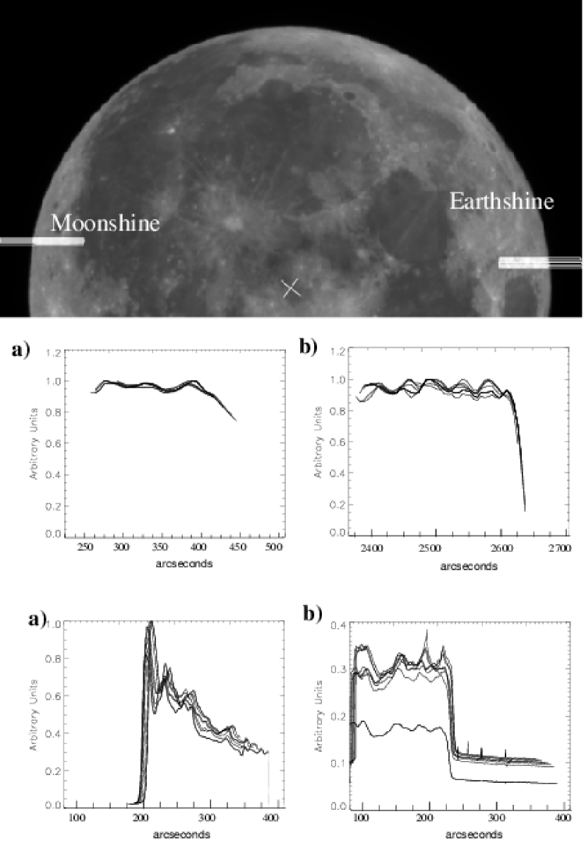
Figure 1: Top: Lunar image taken during the 1993/11/29 eclipse. The MS and ES slit positions during spectroscopic observations on 2003/11/19 are shown for each MS-ES cycle (best visible as eight individual fine white lines just off the limb). Middle: MS (a) and ES (b) limb profiles at lunar phase angle = +1.23^∘, (during eclipse observations) for the slit positions on 2003/11/19. Bottom: (a) MS (showing limb brightening) and (b) ES (showing earthshine flatness on the disk) as actual image profiles along the slit during spectroscopic observations on 2003/11/19 (note that an offset has been introduced in the x-axis). The sharp drops in the middle and bottom occur at the lunar limb. The lower profile at the bottom panel (b) is due to the shorter integration time used during the first exposure.

We observed the spectra of the ES and MS for 2003/11/19, a clear night over Palomar Observatory, between 10.47 to 13.08 hours (UT). We observed with a single order, long slit spectrograph using the Palomar 60^′′ (1.5 m) telescope. An entrance slit of 1.32 arcsec x 6 arcmin on the sky was selected; for comparison, the mean lunar apparent diameter during the time of observations was 32.24 arcmin. This configuration covers the spectral region between 460 nm and 1 040 nm. However this range was limited by the poor CCD quantum efficiency below 500 nm and by the fringe interference patterns in the red, which start to appear at about 800 nm (although they were reduced when taking the ratio ES to MS) but are always important above 980 nm. Thus, the final effective range was limited to between 480 nm and 980 nm.

The slit was EW oriented and positioned in such a way that about half of it was over the lunar disk near the limb, and the other half over the adjacent sky, see Figure 1. Two lunar patches were selected near the bright and dark lunar limbs in the highland regions of the moon. We alternatively measured these patches as the airmass varied through the night. During each MS-ES cycle, the moon was tracked in right ascension and declination at a fixed rate. To account for the moon’s motion relative to the stars, rates were updated every 15 minutes, to minimize the deviation from the original patch. The updates were done after each MS-ES cycle was completed. We obtained a total of 8 MS-ES cycles during observations from moonrise to sunrise.

The basic reduction steps were performed with the Image Reduction and Analysis facility (IRAF) software system. The alignment between the dispersion direction and the CCD rows was verified and the necessary geometrical corrections were applied to all images in order to preserve the maximal possible spectral resolution during the extraction of the spectra; laboratory Argon lamps were used for this purpose, as well as for wavelength calibration.

The spatial profiles within the region covered by the slit for each MS and ES exposure are shown in Figure 1. These profiles are affected by three correctable and/or ignorable types of variations: i) a large gradient due to the overall Lambert-like illumination of the MS, ii) light scattered from the moonshine into the ES (which decreases linearly with the distance to the MS limb), and iii) small features due to the varying reflection index over the lunar surface within the region covered by the slit.

Eight apertures of equal size were initially extracted from every image, four over the sky side and four over the lunar side. The background due to the scattered light was corrected by subtracting a linear extrapolation of the sky spectrum to the position of each of the four ES and MS lunar apertures. The extrapolation was done point by point across the spectral direction. Then, all spectra were normalized to a unit exposure time.

Because moonshine and earthshine exposures were not exactly simultaneous, each MS spectral transmission was interpolated to the airmass of its temporally closer ES spectrum. The ratio ES/MS, $I_{a,\lambda}/T_{a,\lambda}\over I_{b,\lambda}/T_{b,\lambda}$ in Equation 1, could then be calculated to obtain the implied top of the atmosphere ratio.

4 Measuring the lunar relative reflectivity

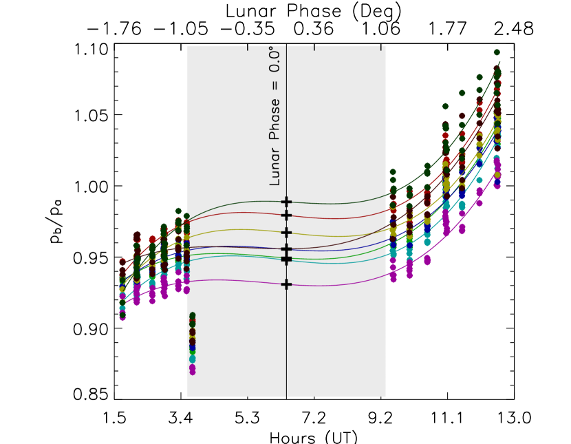
Figure 2: Variation of $\frac{p_{b}f_{b}}{p_{a}f_{a}}$ for all 8 lunar patches (different colors) during 1993/11/29 eclipse. The ratio only takes its textbook meaning when the lunar phase angle is zero. The penumbral shadow region is shaded in the figure, and the best polynomial fit for each patch is also shown. The ratios at lunar phase equal zero interpolated from each fit are given in Table 1. Penumbral shadowing causes one set of points to be well-below the fitted lines.

Table 1: Measured relative reflectivity $p_{b}/p_{a}$ at eclipse totality (lunar phase angle ($\theta$) zero). A standard deviation of about 0.007 resulting from a covariance calculation of the polynomial fit was estimated for each point. The time (UT) at which each ES spectrum was taken and the patch center in selenographic coordinates are also given.

Time (UT)	$lat_{b},\,lon_{b}$	$lat_{a},\,lon_{a}$	$p_{b}/p_{a}$
10.47	-13.3, -82.4	30.2,73.1	0.979
10.89	-12.8, -80.0	31.0,73.7	0.949
11.26	-12.7, -81.5	31.3,71.1	0.947
11.63	-13.6, -79.5	31.9,71.5	0.930
12.02	-13.4, -80.9	31.0,73.7	0.955
12.38	-13.8, -82.0	30.7,73.5	0.967
12.74	-13.2, -78.6	31.5,86.3	0.955
13.08	-13.4, -83.9	31.0,86.3	0.988

To determine the Earth’s reflectance on 2003/11/19, one requires two quantities from observations on other nights – the Moon’s geometrical albedo (determined from total eclipse data) and the lunar phase function (determined over several years of photometric observations, Qiu et al., 2003). To apply these to each of the eight pairs of measurements, one requires the accurate selenographic coordinates for the regions from where the earthshine and moonshine are reflected (Qiu et al., 2003).

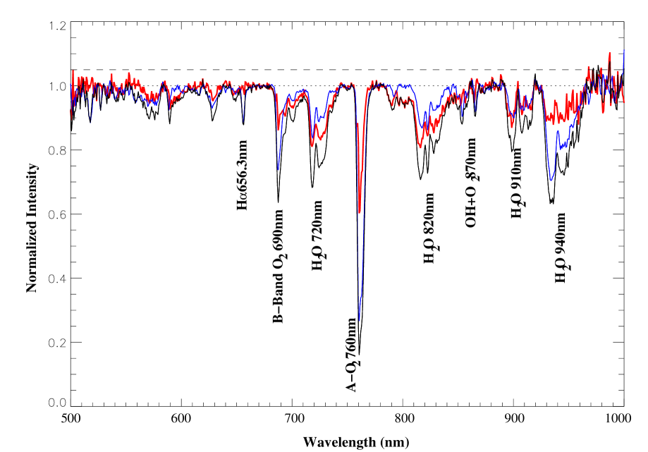
Figure 3: Normalized moonshine spectra (blue), earthshine (black) and their ratio (red) for 2003/11/19. The main gas absorption bands, as well as other features and their central wavelengths are indicated. Note how the solar H$\alpha$ line disappears in the ES/MS ratio.

For each of the eight MS-ES spectral observing pairs, we must re-point the telescope and in the subsequent analysis make a precise, post facto determination of the location of the narrow slit for each observation (rather than always looking at the same fiducial patch, as we do in the photometric observations). We estimate a deviation of up to 10 arcsec in the EW direction and up to 20 arcsec in the NS direction. This assessment is consistent with changes in the slit position shown in Figure 1, (top panel) where each narrow white line (best viewed just off-the-limb) represents the location of spectrograph’s slit for each observation. The magnitude of the changes in the lunar profile observed for different exposures are shown in the same figure for lunar phase +1.23^∘ (middle panel) and lunar phase +117^∘ (bottom panel).

Qiu et al. (2003) argued that the lunar geometrical albedo for the earthshine and moonshine differ by only a small spectral offset, equivalently, we can assume here that $p_{b,\lambda}/p_{a,\lambda}=p_{b}/p_{a}$. In the data reduction, the relative photometric reflectivity of the patches $b$ and $a$ was determined for each of the eight pairs of MS and ES images via a post facto approach to precisely eliminate the error introduced by small deviations from the initial selenographic coordinates (fiducial patch) when re-pointing the telescope for each MS-ES observing cycle. To measure each ratio, $p_{b}/p_{a}$, we used photometric observations of the full moon, interpolating at lunar phase angle $=0.0^{\circ}$ during the lunar eclipse on 1993/11/29. This eclipse was observed during eleven hours (before and after totality) from Big Bear Solar Observatory (BBSO) using the 25 cm solar telescope that is now part of BBSO’s global H$\alpha$ network. Between four and five images were taken, approximately, every 30 minutes. Sixteen lunar patches of 3 arcmin (EW) x 2 arcsec (NS) centered on each ES and MS slit position were selected. The different Earth-Moon distance and lunar polar axis orientation, for the eclipse night and for observations on 1993/11/29 were taken into account. The differences in lunar libration were considered by properly modifying the projected size of the observed patches for each eclipse image. Intensities were normalized to one second exposure and the mean reflectivity for each patch was then calculated to obtain a pair of $p_{b}$ and $p_{a}$ values for each MS-ES observed cycle. Figure 2 shows the variation of the ratio $\frac{p_{b}f_{b}(\theta_{b})}{p_{a}f_{a}(\theta_{a})}$ for each of the eight location pairs corresponding to the eight pairs of observations on 2003/11/19. The location of the pairs and the extrapolated ratios are shown in Table 1. To extrapolate our “$p_{b}/p_{a}$” (quotation marks serve to remind that the ratio is actually defined only for lunar phase angle zero degrees) observations to zero phase angle, a polynomial fit was done for all ratio values just before and after the moon was within the Earth’s penumbral shadow. Note that one set of points does not come close to the curves because this set was taken when the Moon was partly in Earth’s shadow.

For the lunar phase function, we use the values of Qiu et al. (2003) after evaluating the phase function for the bands in Figure 1 and finding that the phase functions are all essentially the same, after removing the ratio $p_{b}/p_{a}$ that provides the overall normalization.

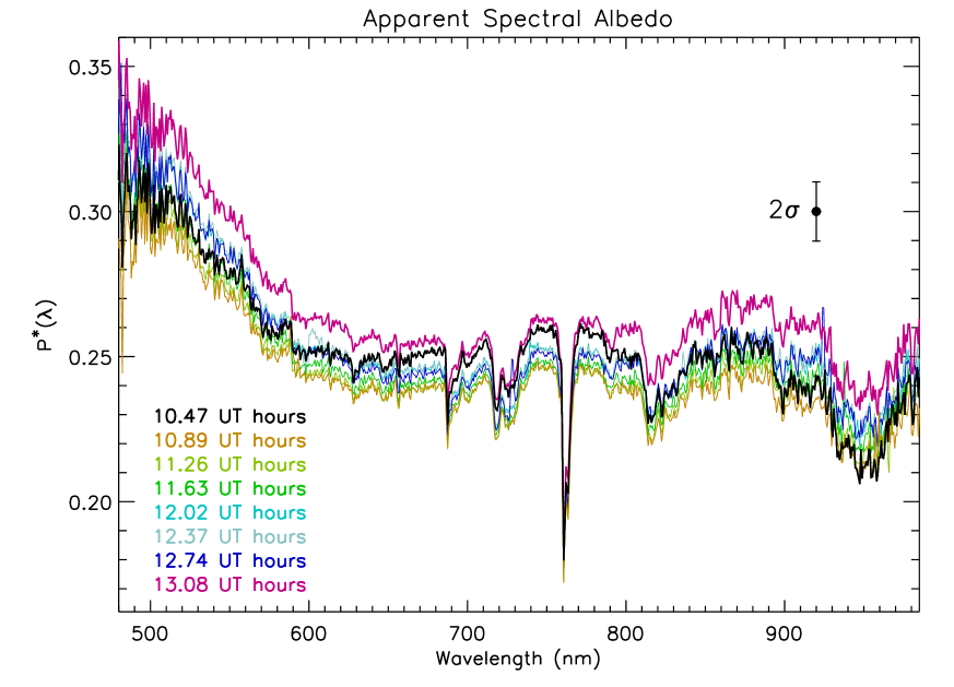
Figure 4: Apparent albedo $p^{*}(\lambda)$ for the night of observations. The main features of the Earth’s reflectance in this region include an enhancement due to the Rayleigh Scattering in the blue, part of the Chappuis O₃ band, which contribute to the drop above 500 nm. Atmospheric absorption bands due to oxygen, as the sharpest A-O₂ at 760 nm, and water vapor are clearly detected. The surface vegetation edge, which is expected to show an apparent bump in the visible albedo above 700 nm is not strong, and neither does it seem to vary appreciably or systematically through the night.

5 Results

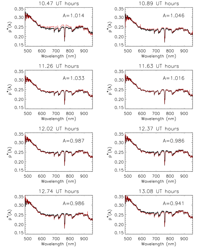
Figure 5: Apparent albedo $p^{*}(\lambda)$ as a function of wavelength taken during the night of observations (red). Also plotted (black) is the mean spectrum for the night, $<p(\lambda)>^{\prime}$, the mathematical average of our eight $p^{*}(\lambda)$ spectra. The averaged spectra, p’ has been artificially displaced by a factor A, also given in each panel, to match the mean value of each $p^{*}(\lambda)$ over the 500-550 nm interval. Note that for the first spectra our observations were centered over Africa (upper left panel), while for the last ones we were monitoring the Amazonian Forest (lower right panel). A deviation from the mean value of up to a 4% in appreciated in the first measurement.

The atmospheric absorption bands in the moonshine spectrum are formed when the moonlight passes through the local atmosphere. The bands in the earthshine spectrum additionally contain the absorption formed when the sunlight passes twice through the global terrestrial atmosphere, on the sunlit part of the Earth, before being reflected from the moon toward our telescope (Montañés Rodriguez et al., 2004). Thus, absorption lines in the ES spectrum are deeper than in the MS spectrum. Since the effect of the local atmosphere is present in both MS and ES, it is removed when the ratio ES/MS is calculated. In Figure 3, the Earth’s atmospheric spectral features, primarily due to molecular oxygen and water vapor, are appreciable for the ES, for the MS and for their ratio. As one would expect, ES features are deeper than MS features whereas lines formed in the solar photosphere, such as H$\alpha$ remain invariant for ES and MS and therefore disappear in the ratio, which further convincing evidence that the last pass through atmosphere is also canceled out in the ratio. Only the cloud patterns in the global atmosphere will affect the shape of the ES/MS spectra by altering the optical path of the ES depending on cloud altitudes and optical thicknesses.

5.1 Nightly spectral albedo

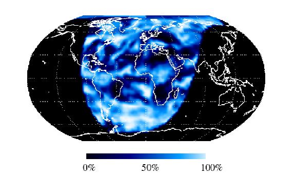
Figure 6: Earthshine-contributing area of the Earth during morning observations from California on 2003/11/19 (10:45-13:10 UT). The superimposed color map represents the mean cloud amount from ISCCP data over this area. Since ISCCP data for 2003 are not yet available, the cloud cover map for 2000/11/19 (closest “equivalent” available) is here shown.

The measured apparent albedos, $p^{*}(\lambda)$, are shown in Figure 4, where different colors indicate its temporal evolution through the night, while different land and cloud distributions move into the sunlit side of the Earth and are visible from the Moon.

During our observing night, we were monitoring the Earth’s spectral reflectance over the area shown in Figure 6. Because ISCCP data are still not updated up to 2003, cloud data for 2000/11/19 were used in the figure for illustration. South America was only partially visible at 10:45 hours, but was near the center of the sunlit area at 13:10 hours. The total covered area during the 2.6 hours of observations, without considering cloud cover, is composed of 79-71% of oceans, 8-11% snow or ice covered areas, and 13-18% of land, 9-14% of which are vegetated areas mainly located in the Amazonian rain forest, Equatorial Africa and Europe. The range of percentages for each surface type correspond to 10:00 and 13:00 UT, respectively.

The possibility of using the red edge signature of vegetation as a tool to detect earth-like extra-solar planets has been discussed in the literature. The red edge has been detected in surface spectral albedo measurements from airplanes at low altitude and from the Galileo spacecraft, all these measurements taken with some spatial resolution. The detected signal shows a step in the Earth’s spectrum starting at about 720 nm, coinciding with an important water absorption band in the atmosphere, and continues to the near infrared (Wendish et al., 2004).

Woolf et al. (2002) observed the earthshine an evening in June 2001 (therefore they were monitoring the Pacific Ocean), and they report an inconclusive vegetation signature above 720 nm, although at the time of their observations no large vegetated area of the globe was visible from the Moon. More detailed observations of the earthshine were undertaken by Arnold et al (2002). They concluded in their study that the vegetation edge was difficult to measure in their earthshine data due to clouds and the effect of atmospheric molecular absorption bands. One of our purposes in this work was to confirm these results and to report any diurnal variability in the vegetation edge or other earthshine signatures, if any.

During the night of 2003/11/19, we find no notable red edge enhancement, even at the times when the South American continent is in full view and in November, when the “greenery” is abundant. This is not a surprise because we should expect that some, if not all, of the vegetated areas contributing to the earthshine to be obscured by the presence of clouds. However, when globally monitoring the Earth, one should note that at all times about 60% of the planet (Rossow et al., 1993) is covered by clouds with a mean global cloud amount variation of about 10% from autumn to spring.

The possibility remains thus, that the whole or large part of the South American continent was covered by clouds at the time of observations, masking any vegetation signal. Mean monthly and annual cloud amounts from ISCCP indicate that this is frequently the case throughout the year (www.isccp.giss.nasa.gov). This could easily be solved by analyzing cloud cover maps for the same night of our observations. If the night of 2003/11/19 had mostly clear skies over that area, then that would imply that the vegetation signal is per se too small to be detected in disk-integrated measurements of earthshine. On the contrary, if it was mostly cloudy, the signal may be strong enough to be detected if clear skies occur over the large enough portion of the rainforests regions of the earth. However, this is not typically the case, as densely vegetated areas are associated with vegetation transpiration and enhanced cloud formation (IPCC, 2001).

The enhancement of the reflectivity in the blue parts of the spectra, below 600 nm, due to the effect of atmospheric gas molecules producing Rayleigh scattering is the most significant feature in our results. The albedo increase toward the blue is consistent with other surface spectral albedo measured from airplanes (Wendisch et al., 2004). From spatially resolved observations and spectral albedo models, a peak at around 310 nm would be expected, if we were covering that spectral region. This is due to the combination of Rayleigh scattering, which decreases as $\lambda^{-4}$, and an ozone absorption.

An enhancement in the 600 to 900 nm region, or else a decrease in the red and blue extremes, of about 4% with respect to its mean spectral value is found when we compare the first spectrum taken at 10.47 hours with the temporal averaged of the eight spectra (Figure 5). As can be seen in the figure, this relative bump systematically changes its curvature through the night (unlike for the 500-600 nm regime), thus we cannot attribute it to any instrumental problem. Since the maximum enhancement is at the beginning of the night, when the sun is still rising in South America, and it almost disappear two hours later, we cannot associate this enhancement with the signal of vegetation neither, which should behave in the opposite fashion. Further, no signal of vegetation is expected below 700 nm. Thus, we associate this variation to the evolution of the surface and cloud pattern over the sunlit Earth during the time of observations.

5.2 Precision of the results

The accuracy of each $p^{*}(\beta,\lambda)$ derived from our earthshine measurements was determined from Equation 1, and depends on the errors in the earthshine to moonshine ratio, the lunar reflectivity (which accounts for the relative reflectivity between two fiducial patches) the lunar phase function (which considers the geometrical dependence of the lunar reflectivity) and the opposition effect coefficient.

The measurement of the earthshine to moonshine ratio, after the sky subtraction and the Beer’s law fitting of the bright side spectra, is the biggest source of error, as occurs in our photometric observations (see Qiu et al., 2003 for details). We estimate it as smaller than 2%. The error derived from the measurement of the (relative) lunar reflectivity was taken as the standard deviation of the polynomial fit to $\frac{p_{b}f_{b}(\theta_{b})}{p_{a}f_{a}(\theta_{a})}$, and has a value of 0.7% from a covariance calculation. The precision achieved for the lunar phase function (and opposition effect coefficient) can be determined down to 0.5%, as report in section 5 of Qiu et al., 2003.

From the propagation of the errors into Equation 1, a standard deviation of the order of 3.7% is obtained for each individual spectral albedo measurement. This is shown in Figure 4 by a two sigma error bar. They are also represented for each data point in Figure 7.

5.3 Comparison with photometric albedos

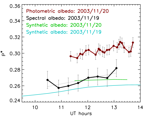
Figure 7: Temporal variation of the spectral albedo averaged between 480 and 700 nm (black solid line). The error bars show the 2 $\sigma$ deviation for each spectral measurement determined from the propagation of errors as discussed in Section 5.2. A linear fit to all points through the night is also shown. The measured apparent albedos from photometric observations for a consecutive night are shown for comparison (red solid line), with error bars also representing twice the standard deviation achieved, but through photometry. Note that the spectral coverage for the photometric albedo is broader (between 400 and 700 nm) than for the spectral albedo. Also plotted are the modeled photometric albedos for 2003/11/19 and 2003/11/20 covering the entire short-wave region through the near IR, using ISCCP data for 2000/11/19 and 2000/11/20 (blue and green). The differences in wavelength coverages probably accounts for much of the offsets.

An evaluation of our results can be done with a comparison to photometric albedo measurements taken simultaneously at BBSO, and with effective albedo simulations for that night following Pallé et al. (2003). To do that, we have averaged in wavelength each spectrum between 480 and 700 nm. Photometric observations from BBSO cover the range between 400 and 700 nm, including a major part of the Rayleigh enhancement. Our simulations, however, cover the entire range of short-wavelength radiation including ultraviolet, visible and near-infrared (spanning 350 to 1500 nm).

Photometric observations at BBSO on 2003/11/19 were taken under a moderately hazy sky, which increases the light scattered by the moonshine and causes a too noisy result for that night; however, on the following night, when the lunar crescent was smaller and the sky conditions clearer, the noise was substantially reduced. The retrieved photometric albedos, the spectrally averaged albedos, and computed photometric models are shown in Figure 7. Both sets of observations were linearly fitted showing a comparable increase from beginning to end of the night.

We regard all of these results as being consistent because of the similarity of the increasing trend and because the offsets are those expected from the different wavelength coverages. In particular, the photometrically observed albedo includes more of the blue and less of the red, which would seem to account for that offset. Further, the simulations include much more of the IR, which roughly puts more weight toward an albedo of 0.25.

6 Conclusions

In this paper, we have accurately determined the Earth’s apparent, global spectroscopic albedo for a single night of November 2003 as measured from Palomar Observatory in California. We show its main spectral features derived from observations of the earthshine spectrum in the visible region. Our results are consistent with simultaneous photometric apparent albedo measurements from Big Bear Solar Observatory covering the same sunlit region of Earth. They are also consistent with our albedo models using cloud patterns for the same day of the year, although for different year due to the, so far, unavailability of the necessary cloud cover data. The comparison with synthetic models of the Earth’s spectrum that take into account a precise cloud cover pattern for the night, and its influence over surface and ocean distribution, will be carried out in future works.

Our measurements do not show any sign of vegetation red-edge, at least for the night of 2003/11/19. If this result were confirmed with the analysis of subsequent earthshine spectra taken at different seasons, and the analysis of simultaneous cloud maps, it would strong limit efforts to use the red-edge as a probe for Earth-like extra-solar planets. We emphasize, however, that other features on the earthshine spectra may still provide a powerful probe.

Observations of the earthshine at different seasons are desirable not only to study other indirect biological signatures, as the seasonal change of global abundances of oxygen, water vapor, carbon dioxide or methane, but also for a better understanding of the influence of these species over the Earth’s albedo and climate.

Results derived from future observations of the earthshine will be invaluable in the search for terrestrial-like extra-solar planets, in particular the search of planetary atmospheres in chemical disequilibrium (as proposed by Hitchcock and Lovelock, 1967). The simultaneous detection of molecular oxygen and methane, for instance, remains a potential biosignature.

References

- Arnold et al., (2002) Arnold L., S. Gillet, O. Lardiere, P. Riaud, and J. Schneider, A test for the search for life on extrasolar planets. Looking for the terrestrial vegetation signature in the Earthshine spectrum, Astronomy & Astrophysics, 392, 231-237, 2002.
- Culf., (1995) Culf A.D., G. Fisch and M.G. Hodnett, The albedo of Amazonian forest and ranch land, Journal of Climate, 8, 6, 1995.
- Goode et al., (2001) Goode, P.R., J. Qiu, V. Yurchyshyn, J. Hickey, M.C. Chu, E. Kolbe, C.T. Brown, and S.E. Koonin, Earthshine observations of the Earth’s reflectance, Geophys. Res. Lett., 28 (9), 1671-1674, 2001.
- Hapke, (1971) Hapke, B., Physics and Astronomy of the Moon, 2nd edition, ed. Z. Kopal, Academic Press, New York, 155, 1971.
- Hapke et al., (1993) Hapke, B.W., R.M. Nelson, and W.D. Smythe, The opposition effect of the moon - the contribution of coherent backscatter, Science, 260, 509-511, 1993.
- Hapke et al., (1998) Hapke, B., R. Nelson, and W. Smythe, The opposition effect of the moon: coherent backscatter and shadow hiding, Icarus, 133, 89-97, 1998.
- Helfenstein et al., (1997) Helfenstein, P., Veverka, J., and Hillier, J., The lunar opposition effect: A test of alternative models, Icarus, 128, 2-14, 1997.
- Hitchcock & Lovelock, (1967) Hitchcock D.R. and Lovelock, J.E., Life detection by atmospheric analysis, Icarus, 7, 149-159, 1967.
- Montañés Rodriguez et al., (2004) Montañés Rodriguez P., E. Palle, P.R. Goode, J. Hickey, J. Qiu, V. Yurchyshyn, M-C Chu, E. Kolbe,C.T. Brown, S.E. Koonin. Advances in Space Research, doi:10.1016/j.asr.2003.01.028, April 2004
- In (2001) Intergovernmental Panel on Climate Change (IPCC), 2001, The Scientific Basis, Contribution of Working Group I to the Third Assessment Report of the Intergovernmental Panel on Climate Change (IPCC), J. T. Houghton, Y. Ding, D.J. Griggs, M. Noguer, P. J. van der Linden and D. Xiaosu (Eds.), Cambridge University Press, pp 944, 2001.
- Palle et al., (2004) Palle E., P. Montañés Rodriguez, P.R. Goode, J. Hickey, J. Qiu, V. Yurchyshyn, M-C Chu, E. Kolbe,C.T. Brown, S.E. Koonin. Advances in Space Research, doi:10.1016/j.asr.2003.01.028, April 2004
- Palle et al., (2003) Pallé, E., P.R. Goode, V. Yurchyshyn, J. Qiu, J. Hickey, P. Montañés Rodriguez, M.C. Chu, E. Kolbe, C.T. Brown, and S.E. Koonin, Earthshine and the Earth’s albedo II: Observations and simulations over three years, J. Geophys. Res., 108(D22), 4710, doi: 10.1029/2003JD003611, 2003.
- (13) Pallé E., P.R. Goode, P. Montañés Rodriguez and S.E. Koonin. Changes in the Earth’s reflectance over the past two decades. Science, 304, 1299-1301, doi:10.1126/science. 1094070, 28 May 2004b.
- Qiu et al., (2003) Qiu, J., P.R. Goode, E. Pallé, V. Yurchyshyn, J. Hickey, P. Montañés-Rodriguez, M.C. Chu, E. Kolbe, C.T. Brown, and S.E. Koonin, Earthshine and the Earth’s albedo I: Earthshine observations and measurements of the lunar phase function for accurate measurements of the Earth’s Bond albedo, J. Geophys. Res., 108(D22), 4709, doi: 10.1029/2003JD003610, 2003.
- Rossow et al., (2004) Rossow, W.B., A.W. Walker, L.C. Garder, Comparison of ISCCP and OTHER Cloud Amounts, Journal of Climate vol. 6, Issue 12, pp. 2394-2418, 1993.
- Wendisch et al., (2004) Wendisch, M., P. Pilewskie, E. Jäkel, S. Schmidt, J. Pommier, S. Howard, H.H. Jonsson, H. Guan, M. Schröder, B. Mayer, Airborne measurements of areal spectral surface albedo over different sea and land surfaces, Journal of Geophysical Research, 109, D08203, doi:10.1029/2003JD004392, 2004.
- Woolf et al., (2002) Woolf N.J., P.S. Smith, W.A. Traub and K.W. Jucks, The Spectrum of Earthshine a pale blue dot observed from the ground, The Astrophysical journal, 574, 430-433, 2002.