Chandra’s tryst with SN 1995N

Abstract

We present the spectroscopic and imaging analysis of a type IIn supernova SN 1995N observed with the Chandra X-ray observatory on 2004 March 27. We compare the spectrum obtained from our Chandra observation with that of the previous observation with ASCA in 1998. We find the presence of Neon lines in the Chandra spectrum that were not reported in the ASCA observation. We see no evidence of Iron in both epochs. The observed absorption column depth indicates an extra component over and above the galactic absorption component and is possibly due to a cool dense shell between the reverse-shock and the contact discontinuity in the ejecta. The ASCA and the ROSAT observations suggested a non-linear behavior of the X-ray light curve. However, with the higher spatial resolution and sensitivity of Chandra, we separate out many nearby sources in the supernova field-of-view that had additionally contributed to the supernova flux due to the large Point Spread Function of the ASCA. Taking out the contribution of those nearby sources, we find that the light curves are consistent with a linear decline profile. We consider the light curve in the high energy band separately. We discuss our results in the context of models of nucleosynthesis and the interaction of the shock waves with the circumstellar medium in core collapse supernovae.

1 Introduction

X-rays from a supernova explosion arise from the interaction of the supersonic ejecta with the circumstellar medium (CSM). The CSM typically consists of a slow-moving wind with the density $\rho=\dot{M}_{\odot}/4\pi r^{2}v_{w}$, where $\dot{M}_{\odot}$ is the mass loss rate, $r$ is the distance from the supernova and $v_{w}$ is the wind velocity. When the ejecta collides with the CSM, it creates two shocks: a high-temperature, low-density, forward-shock ploughing through the CSM (known as blast-wave shock) and a low-temperature, high-density, reverse-shock moving into the expanding ejecta. Initially the X-rays come from the forward-shocked shell dominated by continuum radiation, but later on X-rays arise also from the reverse-shock, which can have substantial line emission, thus providing nucleosynthetic fingerprints of the ejecta. The temporal evolution of the X-ray luminosity of a supernova can yield information on the density distribution in the outer parts of the exploding star ($\rho\propto r^{-n}$, here $n$ can be in the range $7-12$, typically $n\sim 10$ for a Blue Supergiant (BSG) and $n\sim 12$ for a Red Supergiant (RSG)- see Chevalier & Fransson (2003)). These studies therefore are of interest from the stellar structure and the evolutionary point of view.

SN 1995N was discovered in MCG-02-38-017 (Arp 261) on 1995 May 5 (Pollas, 1995) at a distance of 24 Mpc (see Fransson et al. (2002)). Pollas (1995) estimated that the supernova was at least 10 months old upon discovery, by comparing with spectroscopic chronometers. We assume the date of explosion to be 1994 July 4 throughout the paper. To date twenty-two supernovae have been detected in the X-ray bands and SN 1995N appears to be at the high end of the X-ray luminosity (Fox et al., 2000), which makes it suitable for study in the X-ray wave bands even at late stages. Additionally, SN 1995N is one of the only six supernovae of type IIn from which X-ray emission has been observed; the others are SN 1978K (Schlegel et al., 2004), SN 1986J (Schlegel, 1995), SN 1988Z (Fabian & Terlevich, 1996), SN 1998S (Pooley et al., 2002) and SN 2002hi (Pooley & Lewin, 2003).

Nomoto et al. (1996) have suggested a continuum of merged stars in binary systems with different common envelope masses as possible progenitors of various types of supernovae, in particular types IIL, IIb and IIn. The evolutionary path of a close binary system depends upon the initial mass ratio $q_{0}$ ($=m_{2}/m_{1}$, where $m_{2}$ is the less massive secondary star and $m_{1}$ is the more massive primary star) and on their initial separation $a_{0}$. If the initial mass ratio is $q_{0}\leq 0.4$, the mass transfer is highly non-conservative and leads to the formation of a common envelope and the subsequent spiral-in of the secondary towards the core of the primary. The structure of the CSM from the spiral-in may be asymmetric, where the ejected mass may form a bipolar jet or a disk-like structure. When the stellar core collapses and explodes, the supernova lights up the slow-moving gas into narrow emission lines leading to the type IIn supernova classification (n for narrow emission line). Type IIn supernovae show unusual optical characteristics and are known to span a very broad range of photometric properties such as decline rates at late times (Filippenko, 1997). It is likely that these differences are related to their progenitor’s structure, mass, composition as well as the composition and the density profile of the CSM (Li et al., 2002). These supernovae show the presence of strong, narrow Balmer line emission on top of the broader emission lines in their early spectra. It is believed that the narrow emission lines originate in the dense and ionized circumstellar (CS) gas (Henry & Branch, 1987; Filippenko, 1991). The presence of strong H$\alpha$ emission line, the high bolometric luminosity and the broad H$\alpha$ emission base powered by the interaction of the supernova shock with the CSM, all point towards a very dense circumstellar environment (Chugai & Danziger, 2003). This interaction of the supernova shock with the dense CS gas is indicated by strong radio and X-ray emission detected from several type IIn supernovae and in particular SN 1995N. Optical and ultraviolet observations of SN 1995N (Fransson et al., 2002) upto about 1800 days after the explosion, revealed three distinct velocity components. Narrow lines from the CS gas show both low and high ionization states and are caused by photo-ionization of the CS by X-rays from the shock. The intermediate component has a velocity of $2500-5000$ km s^-1, and is dominated by the newly processed Oxygen that is conjectured by Fransson et al. (2002) to be a part of the unshocked (by the reverse-shock) ejecta. The broad component whose extended wings reach $\sim 10,000$ km s^-1 is dominated by lines of HI, HeI, MgII, and FeII.

Apart from the narrow lines of H$\alpha$ mentioned above, SN 1995N showed narrow lines of several other elements in multiple charge states. In particular, the intensity ratios of narrow Oxygen lines suggested a high electron density, $n_{e}\geq 10^{6}\rm cm^{-3}$ (Garnavich & Challis, 1995). SN 1995N has turned out to be relatively bright in all the wavebands. It has been detected in radio wave bands with the VLA (Van Dyk et al., 1996) and the Giant Metrewave Radio Telescope (GMRT) (Chandra & Ray, 2005). In X-ray wave band, it has been detected by ROSAT in August 1996 and in August 1997 and later by ASCA in January 1998 (Fox et al., 2000). The ROSAT observations showed a 30% decline in the X-ray flux from August 1996 to August 1997, whereas the ASCA observations showed a rise by a factor of two in between August 1997 to January 1998 (see Table 1). To address the question of non-steady decline of the luminosity unequivocally, however, it is important to spatially resolve the field of view (FoV) around SN 1995N to an accuracy substantially larger than the ASCA angular resolution. If this trend is indeed real, it could have very interesting implications for the supernova. It could imply that the X-ray emission may be coming from the clumpy clouds crushed by the forward-shock or it could show the inhomogeneity in the reverse-shock itself. Fig. 1 illustrates two different scenarios of the X-ray emission: one due to the emission from the reverse-shock heated ejecta, which predicts linear decline in luminosity light curve, and the other due to slow shocks in the CSM clumps, predicting bumps in the light curve.

SN 1995N has declined very slowly in the optical band (see Li et al. (2002) and references therein), with only a 2.5 mag change in the V-band over $~{}2500$ days after explosion. This is consistent with the slow spectral evolution reported in Fransson et al. (2002). Ground based optical and HST observations of the late-time spectral evolution of SN 1995N were used by Fransson et al. (2002) to argue that the late-time evolution is most likely powered by the X-rays from the interaction of the ejecta and the circumstellar medium of the progenitor. They in turn proposed that the progenitors of type IIn supernovae are similar to red supergiants in their superwind phases when most of their hydrogen-rich gas is expelled in the last $10^{4}\,\rm yr$ before explosion.

We observed SN 1995N under Cycle-5 Chandra Guest Observation program for 55.74 ks exposure time on 2004 March 27 with ACIS-S3. In this paper we present the analysis and interpretation of the data and their implications. Section 2 deals with the observation and data analysis. In Section 3, we present the results of spectroscopic and imaging analysis. Section 4 gives a discussion of the results and Section 5 presents a summary.

2 Observations and data analysis

We observed SN 1995N from 2004 March 27 UT 17:55 to 2004 March 28 UT 10:00 with the Advanced CCD Imaging Spectrometer (ACIS-S) instrument of Chandra X-ray observatory as a part of GO observations (Obs ID 5191). The CCDs S2, S3, I2 and I3 were switched on for the observations with aim point on the back-illuminated chip S3. The back-illuminated chip has an advantage of relatively flat spectral resolution over the front-illuminated chips. The observation was taken in very faint (VF) mode. The total exposure on the source was 55.74 ks. The summary of the Chandra observations along with all previous X-ray observations of SN 1995N are provided in Table 1.

The data were analyzed using CIAO analysis threads and XSPEC (Arnaud, 1996). Event-2 files (pipeline processed files) were used for the data analysis. In order to check for any X-ray flaring events, we selected a background region of size 87^′′, carefully excluding point sources. We then obtained the light curve of this selected background region using “dmextract” and CIAO-script “analyze_ltcrv.sl”. We did not find any flaring and the data were quite clean and contained no spurious background events.

We then extracted the SN1995N events in a radius of 7^′′ centered at SN1995N’s position. The total counts for the source events was 758 and the observed count rate was $0.0138\pm 0.0026$ cts/s. We also extracted an annulus of inner radius of 7^′′ and outer radius of 22^′′ centered at the supernova position to obtain the background counts. We then generated the “pulse invariant” spectra for the source and the background events using “dmextract”. The response matrices were constructed at the position of SN 1995N. We corrected the response matrix in order to take into account the contamination due to the ACIS quantum efficiency degradation at low energies. To generate the response matrices (RMF and ARF), we used the CIAO threads: “acis_fef_lookup”, “mkrmf”, “asphist”, and “mkarf”.

2.1 Data Analysis: Spectral lines

We binned the data in 20 cts per channel for the spectral analysis using the HEASARC tool “GRPPHA”. We used the XSPEC software for the spectral fitting of the data. We ignored the counts below 0.3 keV and above 7.5 keV. This is because there was almost no flux in this energy range and the Chandra response is quite poor at these energies. We modeled the background with a best-fit broken powerlaw model with a break at an energy 2.7 keV, and remove its contribution from the source spectrum. Table 2 gives the best-fit parameters for the background model.

2.2 Imaging Analysis

We imaged the field of view of the SN 1995N. We used only the S3 chip for imaging, the aim point for SN 1995N. We did not apply the CTI (Charge Transfer Inefficiency) correction to the data because S3-back illuminated chip is not significantly affected by this effect. Also we did not have enough counts to be able to see this tiny correction factor. We built the relevant instrument map for the data using mkinstmap and then generated the spectrally weighted exposure map using mkexpmap. This file was generated using the CIAO-script “spectrum.sl”. The event-2 image divided by the exposure map gives the corrected image. We also ran “wavdetect” to detect the faint sources in the field of view.

3 Results: X-ray spectra and High Resolution Image

3.1 Spectral fits to the data: line emission

While fitting the source data models in our Chandra spectrum, we initially fixed the background to the values derived in Section 2.1 (Table 2), and later, while doing the final iteration, we allowed these parameters to vary to get the real estimates on the errors of the source model parameters. First we fit the continuum thermal bremsstrahlung model including the galactic absorption. This fit is certainly not a good fit. The spectral shape suggests the possibility of a line around 1 keV. We then add a Gaussian component at 1 keV and refit the data. The fit improves with the total ${\chi}^{2}$ changing by 18, so the line parameters have a confidence level of 99.9%. The best-fit line energy is 1.02 keV. We fit the Gaussian with its line width fixed at zero. When allowed to vary, the line width remains close to zero within the errors because the ACIS resolution is insufficient to resolve the line. We further note the possibility of another line around 0.9 keV. Since both the lines are very closely spaced in energy, it is difficult to fit both the lines together. Therefore, fixing the parameters of the Gaussian already fit at 1.02 keV, we add another Gaussian at 0.9 keV, again with the line width of the Gaussian fixed to zero. The $\chi^{2}$ improves by 5, significant at 90% level for 2 parameters of interest (line position, normalization). The best-fit line energy is 0.85 keV. Although this is not a very robust detection, we suggest the possible identification of this line as Ne IX. Alternatively, it could be a signature of the Ne I K-edge. In Table 3, we report the best-fit values for the various models. In Table 3 the best fit $\chi^{2}$ is obtained for the reported parameters of Bremsstrahlung model ($kT=2.35\,{\rm keV}$, $N_{H}=1.51\times 10^{21}$ cm^-2) with only 2 Gaussian components. The data and our model are shown in Fig. 2. The corresponding confidence contours of the line at 1.02 identified as NeX K-$\alpha$ line are shown in Fig. 3 and this line is very well constrained in the line centroid and normalization. Fig. 4 shows the confidence contours for the line at 0.85 keV, demonstrating that the line is reasonably constrained at the 90% confidence level in the centroid and normalization. We also plot the confidence contours of galactic absorption versus the bremsstrahlung temperature. Both the parameters are well constrained (see Fig. 5).

We tried to fit other lines as well but we obtained only the upper limits, and our fits did not improve significantly via a change in $\chi^{2}$. Table 4 gives the upper limits on O, Mg, Si, S and Fe lines. Only Si line at 2 keV shows little significance; however, when we plot the confidence contours for Si line, the lower bound of the line is completely unrestricted even at 90% level. Fig. 6 shows the confidence contours for Si line, which clearly rules out the possibility of presence of the Si feature at 2 keV.

We also applied the VMekal model to the spectrum. ‘VMekal’ is a model in the XSPEC for an optically-thin thermal plasma model developed using codes of Kaastra (1992); Mewe et al. (1985, 1986); Liedahl et al. (1995). The ‘L’ in ‘Mekal’ refers to the iron L shell corrections to the codes from Liedahl et al. (1995). We fit a model to the spectrum with a fixed hydrogen density of $2\times 10^{6}\,{\rm cm^{-3}}$, with a solar abundance. We find that the VMekal model fits are least sensitive to the hydrogen density. Here the abundances of C, N, Na, Al, Ar, Ca and Ni were fixed to the solar abundance. We separately let the abundances of O, Mg, Ne, Si, S and Fe vary. Only the abundance of Ne and Si are significant with respect to solar (see Table 3 and 4). The enhanced Ne is consistent with the results obtained from the bremsstrahlung plus Gaussian fit, so we identify the 1.02 keV emission as Ne X. The presence of the Si line is ruled out from the confidence contour plot as discussed. Table 4 show the upper limits on the abundances of various lines. The best fit column depth and temperature in the VMekal fit are: $N_{H}=(3.71\pm 2.79)\times 10^{20}\,{\rm cm^{-2}}$ and $kT=3.03$ keV.

Based on $\chi^{2}$ arguments, the bremsstrahlung plus two Gaussian model provides a better fit to the data than VMekal model fit. Table 3 provides the best-fit parameters for the VMekal. Fluxes predicted by various models extrapolated to the ROSAT (0.1-2.4 keV), and ASCA (0.5-7.0 keV) bands are given in Table 5. The fluxes quoted here are absorbed fluxes. It is noticeable that in both the models, the fluxes predicted are quite similar to each other.

The value of best fit absorption column density in Bremsstrahlung model is $N_{H}=1.51\times 10^{21}\,{\rm cm^{-2}}$. From the galactic extinction maps, we get $E_{B-V}=0.1158$ for SN 1995N coordinates, which gives galactic absorption $N_{H}=5.3\times 10^{21}E_{B-V}$, using the relation of Predehl & Schmitt (1995), to $6.1\times 10^{20}\,{\rm cm^{-2}}$. The latter is about two and a half times smaller than the value we obtain from the model fits. We tried to fit the above models again by fixing the galactic absorption to be $6.1\times 10^{20}\,{\rm cm^{-2}}$. Our results were much worse than the previous fits. Table 3 gives best-fit parameters for the model fit when $N_{H}$ is fixed to $6.1\times 10^{20}{\rm cm^{-2}}$. Here we mention that the $N_{H}$ determined from radio measurements of the galactic 21-cm line (Dickey & Lockman, 1990) is $7.8\times 10^{20}{\rm cm^{-2}}$, which is consistent with the $N_{H}$ determined from optical extinction (see $N_{H}$ from HEASARC page). We considered the possibility that the extra column depth in our best fit models is due to the interstellar medium of the host galaxy. However, the Bremsstrahlung or powerlaw models fitted to sources other than SN 1995N in the field of view of ACIS yield a column depth of $N_{H}=6.97\times 10^{20}\;{\rm cm^{-2}}$ (see Section 3.2), which is same as that obtained from galactic extinction calculations. This implies that there is almost no extra absorption due to the interstellar medium of the host galaxy. Therefore the excess $N_{H}$ seen in the Chandra spectrum of SN 1995N over the galactic and host galaxy column depth is most likely in the SN itself, due to the cool ejecta shell formed after the passage of the reverse-shock through it inwards of the contact discontinuity. If the extra absorption layer ($N_{H}=1.5\times 10^{21}\;\rm cm^{-2}-6\times 10^{20}\;\rm cm^{-2}=9\times 10^{20}\;\rm cm^{-2}$) were located deep in the He layers near the external boundary of the C+O core, with a characteristic expansion velocity of $5000\,\rm kms^{-1}$ (seen in the Oxygen rich layers in the Optical/UV bands by Fransson et al. (2002)); then the upper limit to the mass swept-up in the cool shell is (Chevalier & Fransson (2003)):

$$M_{rev}=N_{cool}4\pi R_{s}^{2}m_{p}(X_{O}^{\odot}/X_{O}^{sh})=2\times 10^{-3}M_{\odot}$$

since it is the Oxygen abundance of the gas ($X_{O}^{sh}/X_{O}^{\odot}=100$) that mainly contributes to the X-ray absorption near 1 keV. If the cool shell is well into the helium rich layers, then the implied mass in the absorption shell is considerably larger ($\sim 0.8M_{\odot}$).

3.1.1 Density and ionization state of the radiating plasma

An important question in studying the radiative properties of an ionized plasma is the mechanism of ionization, which we shall discuss elsewhere (paper in preparation). The strengths of the Ne X line reported in section 3.1 (see Table 3) allow us to deduce whether the plasma is in an equilibrium ionization state. The relaxation time for a particular ion, $t_{rel}$ is minimum of the ionization time ($t_{ion}=[C(T_{e})n_{e}]^{-1}$) (Mewe, 1999) and recombination time ($t_{rec}=[\alpha(T_{e})n_{e}]^{-1}$), where $C(T_{e})$ and $\alpha(T_{e})$ are the collisional ionization and recombination coefficients, and $T_{e}$ is the electron temperature. The re-ionization parameter is given by (Verner & Ferland, 1996)

$$\alpha(T_{e})=a[(T_{e}/T_{0})^{1/2}(1+(T_{e}/T_{0})^{1/2})^{1-b}(1+(T_{e}/T_{1})^{1/2})^{1+b}]^{-1}$$ (1)

where $a$, $b$, $T_{0}$ and $T_{1}$ are best-fit parameters, obtained from Verner & Ferland (1996) for Ne X, and leads to a recombination parameter $\alpha(T_{e})=2.8\times 10^{-13}\,{\rm cm^{3}\,s^{-1}}$. Hence $n_{e}t_{rel}={\rm min}(1/C(T_{e}),1/\alpha(T_{e}))=1.32\times 10^{12}\,{\rm cm^{-3}\,s}$.

For a steady state ionization to hold, the relaxation time for ionization should be shorter than the local cooling and the expansion times. The cooling timescale $t_{cool}$, given by: $n_{e}t_{cool}=3kT/\Lambda$, where $\Lambda$ is cooling function, can be obtained from McCray (1987) :

$$\Lambda=1.99\times 10^{-23}T_{7}^{-0.7}+7.27\times 10^{-25}T_{7}^{-1/2}\,{\rm ergs\,cm^{2}\,s^{-1}}$$ (2)

where $T_{7}$ is the temperature in $10^{7}$ K. Hence we get $\Lambda=1.03\times 10^{-23}\,{\rm ergs\,cm^{2}\,s^{-1}}$. Therefore $n_{e}t_{cool}=1.1\times 10^{15}\,{\rm cm^{-3}\,s}$, approximately the same as the corresponding hydrodynamic timescale parameter and which is much larger than the relaxation time. Hence the plasma is in ionization equilibrium, which is expected for a high-density young supernova. We note that the above analytical expression for cooling does not hold for non solar composition. However, Nymark, Fransson and Kozma (private communication) have shown that the equilibrium is nevertheless expected, except for low temperature shocks and shocks in medium highly enriched in heavy elements (e.g. oxygen) and equilibrium does not hold good for lines with $h\nu\leq 0.1$ keV.

3.1.2 Line luminosity, Neon mass and the location of the emitting gas

The line luminosity for a given line can be given as volume integral of its emissivity. For NeX line:

$$L_{NeX}=\eta\int\int j_{NeX}{\rm d}\Omega{\rm d}V$$ (3)

where $\eta$ is a cascade factor that denotes the fraction of recombinations that leads to emission of the Lyman $\alpha$ line in Neon. $\eta$ is at least 0.13 (the number of direct recombinations to ($n=2\,^{2}P$) excited state is typically 13% of total, – see Osterbrock (1989) Table 2.1) and ranges up to about $\sim 50\%$ for all final states except the ground state (we assume $\eta=0.4$). From Table 3, the line strength of Ne X ($3.4\times 10^{-6}\,{\rm photons\,cm^{-2}\,s^{-1}}=5.6\times 10^{-15}\,{\rm ergs\,cm^{-2}\,s^{-1}}$) leads to $L_{NeX}=3.9\times 10^{38}\,{\rm ergs\,s^{-1}}$ at SN 1995N distance (24 Mpc). Emissivity for Ne X can be given as

$$j_{NeX}=n_{e}n_{NeXI}\alpha_{NeX}^{eff}\frac{h\nu_{NeX}}{4\pi}$$ (4)

Let us assume $n_{Ne~{}XI}$ is a fraction $f$ of total $n_{Ne}$ i.e. $n_{Ne~{}XI}=f\;n_{Ne}$. If most of the Ne is in the Helium zone close to the C+O core boundary, (see the Discussion section) then with $n_{Ne}=6.65\times 10^{-4}\,n_{He}$ (see Woosley et al. (2002), Fig. 9 for a 15 $M_{\odot}$ star) and $n_{e}=2n_{He}$, the emissivity of Ne X (see the above two equations) gives:

$$\eta\int n_{e}^{2}{\rm d}V=\eta\frac{4\pi R^{3}}{3}n_{e}^{2}=\frac{6.41\times 10^{63}}{f}\,\rm cm^{-3}$$ (5)

The first equality assumes that the gas is uniformly distributed. Since the velocity at Oxygen layer is 5000 km/s, the velocity of the Neon has to be greater than this if the Neon is in the Helium layers. Hence for the present epoch, we assume $R=vt=1.57\times 10^{17}(v/5000\,{\rm km\,s^{-1}})\,(t/10\,{\rm yrs})$. Therefore

$$n_{e}=\frac{6.77\times 10^{5}}{\sqrt{f}}\,{\rm cm^{-3}}$$ (6)

The ionization potentials of all ionized Neon species upto Ne VIII are less than 240 eV, whereas those of Ne IX and Ne X are above 1195 eV. Hence at such high temperatures as found by our Chandra observations, the predominant species of Neon are expected to be Ne X and Ne XI. This is also indicated by the clear detection of spectral lines of Ne X and a possible detection of Ne IX. Thus we expect that the fraction of Ne XI will be significant, i.e. $f=n_{Ne~{}XI}/n_{Ne}\geq 0.1$. For $f=0.1$, $n_{e}=2.1\times 10^{6}\,{\rm cm^{-3}}$, and $n_{He}=n_{e}/2=1.0\times 10^{6}\,{\rm cm^{-3}}$, which gives $n_{Ne}=687\,{\rm cm^{-3}}$. The corresponding mass of Ne, measured from the above Ne density, is $0.16(f/0.1)^{-1/2}M_{\odot}$. Note that the implied number density of the electron is not so sensitive a function of the ionization fraction of $Ne_{XI}$.

Table 6 gives theoretical estimates by Woosley et al. (2002) of elements synthesized in inner zones of massive stars which can be compared with our estimate of the Neon mass detected in SN 1995N. However, the Neon mass estimated in the previous paragraph is an overestimate due to two reasons: firstly, the Neon is confined mainly in a thin layer, with a shell of thickness $\Delta r$, and not in the entire total volume inside the reverse shock; secondly, we have assumed a constant density in the shell, whereas, the density is a function of radius (velocity) as: $\rho\propto(1/t^{3})r^{-n}$ ($n\leq 8$ for adiabatic shock). The Neon layer lies between Oxygen (velocity $\sim 5000\,{\rm kms^{-1}}$) and Hydrogen-Helium zone (velocity $\sim 10,000\,{\rm kms^{-1}}$), i.e. in a mass shell of 3.05 $M_{\odot}-$4.1 $M_{\odot}$ for a 15 $M_{\odot}$ star (see Table 6). Hence, the Neon mass depends on the velocity at which it occurs as:

$$\int\rho dV\propto\int(1/t^{3})r^{-n}\,4\pi r^{2}dr=K\int^{v_{1}}_{v_{2}}v^{-n+2}dv$$

This velocity dependent factor reduces by $\approx$ 30 from the Oxygen layer to the Hydrogen-Helium layer boundary for $n=8$. Hence the actual mass of Neon is likely to be at least an order of magnitude lower than $0.16M_{\odot}$ estimated above or about $5\times 10^{-3}M_{\odot}-1\times 10^{-2}M_{\odot}$. This is consistent with Neon being in the Helium layer for a $15M_{\odot}$ star (see row 3 of Table 6). We find that for other stellar masses and other composition zones, the required Neon mass is much larger than observed. Therefore, Neon in the Helium core of the $15M_{\odot}$ star is the probable site where it was co-synthesized with C, N, and He.

3.2 Imaging the SN 1995N Field of View

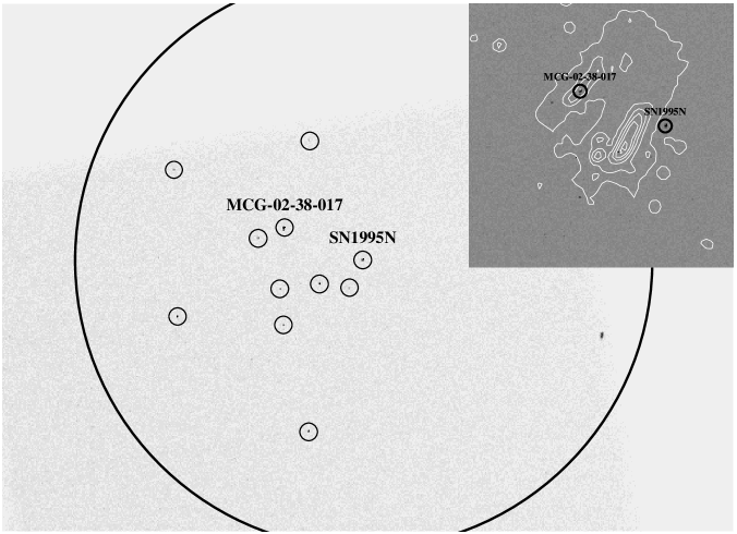
Fig. 7 inset shows the part of the SN 1995N FoV with optical contours overlaid. The positions of SN1995N and the galactic center of MCG-03-38-017 are also shown in Fig. 7. The nearest detected source from the supernova at RA= $14^{\mathrm{h}}49^{\mathrm{m}}29\fs 09$, and Dec= $-10\arcdeg 10\arcmin 37.38\arcsec$ at a distance of $26\arcsec$, is 20 times less bright (count rate of 0.0007 cts/s) than the supernova. Thus, the resolution and sensitivity achievable by the Chandra are crucial to the proper measurement of the SN 1995N flux in this complex field.

We note that in the ASCA observations, the supernova counts were extracted from a circle of radius 4$\arcmin$ centered on the supernova position (Fox et al., 2000), excluding the counts in a circle of radius 1.5$\arcmin$ centered on source “A” (shown as the non-circled source at the extreme right edge in Fig 7). Fig. 7 shows the Chandra ACIS S3 image with a circle of radius 4$\arcmin$ centered on SN 1995N. It is evident from the figure that even after excluding source “A”, there are many other sources within the 4$\arcmin$ circle that must have contributed towards the supernova flux, including the parent galaxy MCG-02-38-017. ROSAT-HRI had sufficient resolution to detect these sources. But due to its high instrumental background, it could detect only two sources apart from the SN, in the 4$\arcmin$ circle as opposed to 10 sources in Chandra observations. The sources detected by ROSAT-HRI were galactic center (0.0009 cts/s) and the source ”A” (0.0025 cts/s). The corresponding SN counts in the Aug 1996 ROSAT observation were 0.009 cts/s. In our Chandra observations, we extracted the counts from all the sources in HPD of 4$\arcmin$ and fit the Bremsstrahlung and power-law models to the summed spectrum assuming all the sources in 4$\arcmin$ radius as a single source (excluding the source “A”). Since the power-law model fits gives a better ${\chi}^{2}$ (model parameters: $\gamma=2.14^{+0.10}_{-0.15}$, $N_{H}=6.97^{+2.4}_{-3.3}\times 10^{20}\,{\rm erg\,cm^{-2}\,s^{-1}}$), we adopt power-law model. The observed counts of the combined sources is 2328, whereas the total counts for SN 1995N is 758. This means that if we were to include all these sources, we would have over-predicted the supernova flux by a factor of 3 at the Chandra epoch.

3.3 X-ray light curve of SN 1995N

Since the supernova was observed with the ROSAT in 1996 and 1997 and with the ASCA in 1998, we construct the light curves over an interval of 8 years. Fig. 8 shows the light curves for the unabsorbed fluxes at soft (ROSAT) energies (0.1-2.4 keV) and at hard (ASCA) energies (0.5-7.0 keV). The ROSAT HRI fluxes were determined by Fox et al. (2000) using the ASCA spectrum. We re-determined the ROSAT fluxes and their uncertainties (ranges) from the ASCA spectrum (see Table 1). Although the fluxes remain identical, the uncertainties increased by a small amount, particularly for the high-energy bands. To calculate the unabsorbed flux, we fixed the galactic absorption to zero and calculated the fluxes in the above two bands. The light curves show that the ASCA flux is well above all the other flux measurements. Without the ASCA point and only with the ROSAT and Chandra data points, a consistently declining trend in the flux is apparent. If the trend is truly linear, then the expected flux at the ASCA epoch should be $\sim 6\times 10^{-13}\,{\rm erg\,cm^{-2}\,s^{-1}}$ in the 0.1-2.4 keV band and $\sim 8\times 10^{-13}\,{\rm erg\,cm^{-2}\,s^{-1}}$ in the 0.5-7.0 keV band, approximately a factor of 1.6 below the observed ASCA data points (Fig. 8). However in the Section 3.2, we have shown that due to the large half-power diameter of the ASCA mirror system, the measured flux of SN 1995N in January 1998 measurement was subject to contamination from the other luminous X-ray sources contained within the angular footprint of the ASCA. Since our Chandra image identified and measured the fluxes from these sources, we can evaluate the apparent non-linear behavior of the light curve.

We find from the Section 3.2 that if we assume that the X-ray flux of the combined sources remained constant with time, then it explains most of the ASCA flux excess, from that of the predicted one from the linear extrapolation between ROSAT and Chandra points, shown in Fig. 8. The unabsorbed flux from the Chandra spectrum in the 0.1-2.4 keV band in a circle of HPD 4$\arcmin$ (excluding source “A”), is $(2.94\pm 0.34)\times 10^{-13}\,{\rm erg\,cm^{-2}\,s^{-1}}$. Since we know that the contribution of the supernova flux is $(0.85\pm 0.20)\times 10^{-13}\,{\rm erg\,cm^{-2}\,s^{-1}}$ in this band, the excess flux due to the rest of the sources at present is $(2.09\pm 0.39)\times 10^{-13}\,{\rm erg\,cm^{-2}\,s^{-1}}$. Similarly in the 0.5-7.0 keV energy range, the unabsorbed flux in the 4$\arcmin$ radius is $(3.15\pm 0.36)\times 10^{-13}\,{\rm erg\,cm^{-2}\,s^{-1}}$. Excluding the supernova contribution in this higher energy band, i.e., $(1.05\pm 0.25)\times 10^{-13}\,{\rm erg\,cm^{-2}\,s^{-1}}$, the flux of the rest of the sources is $(2.11\pm 0.44)\times 10^{-13}\,{\rm erg\,cm^{-2}\,s^{-1}}$ at present. If we assume that the flux of all these sources remained constant from the ASCA epoch to the present Chandra epoch, then we can subtract this contribution from that of the ASCA measurement of the supernova, to estimate the actual contribution due to the supernova only. By this method the supernova flux at the ASCA epoch in 0.1-2.4 keV band is $(6.9\pm 1.6)\times 10^{-13}\,{\rm erg\,cm^{-2}\,s^{-1}}$ and in the 0.5-7.0 keV band, it is $(10.5\pm 0.7)\times 10^{-13}\,{\rm erg\,cm^{-2}\,s^{-1}}$. Fig. 8 shows that in the 0.1-2.4 keV band, the ASCA corrected flux falls on the light curve within the error bars but the discrepancy is larger at 0.5-7.0 keV. Thus the soft band light curve appear consistent with a linear decline, including the ASCA January 1998 measurement. However there appeared to be a possibility that there was an extra flux in the hard X-ray band.

We also plot the de-reddened V-band optical light curve (Li et al., 2002) and H$\alpha$ light curve (Fransson et al., 2002) along with the X-ray decline rate (see Fig. 8). Here, $A_{V}=3E_{B-V}=0.3474$. H$\alpha$ light curve dominates over the V-band light curve until $\sim 1200$ days since explosion. Both V-band and H$\alpha$ fluxes are much lower than X-ray fluxes.

3.4 Hard X-ray excess in the ASCA era?

There could be a few possible scenarios to explain this excess of the hard X-ray flux.

1. It is possible that the supernova flux had really increased at the ASCA epoch, and the increase was essentially in the hard X-rays. In that case, it is a physically interesting feature and could be due to the dense clumps from the ejecta being hit by the reverse-shock. Alternatively, it could be due to an inhomogeneous CSM being hit by the blast-wave shock.

2. Another possible explanation could be that our assumption about the sources within the 4$\arcmin$ FoV of the supernova being constant in time is incorrect. It is quite possible that one or more of these sources are time variable, such as X-ray binaries, and most of their flux fall in the hard X-ray band. We estimate, that to explain the excess flux of $\sim 2\times 10^{-13}\,{\rm erg\,cm^{-2}\,s^{-1}}$ in the $2.4-7.0$ keV band (as described in last section) in January 1998 ASCA observation over a linear decline between 1996 and 2004, a typical X-ray binary contributing roughly 1000 counts is required. This corresponds to a count rate increase of $\sim$0.02 counts s^-1 in the Bremsstrahlung model with $kT=3.32\pm 0.36$ and $N_{H}=(8.42\pm 1.40)\times 10^{20}\,{\rm cm^{-2}}$. Hence, such variability in one X-ray binary can explain the excess ASCA hard band flux. A detailed analysis of the sources in the Chandra FoV, other than SN 1995N is in progress and will be reported elsewhere (Sutaria et al., in preparation).

3. In this scenario, we note that for the ASCA analysis of the supernova spectrum, the circle of 4$\arcmin$ HPD was chosen for the supernova counts and then the contribution of source “A” was corrected by excluding the counts from the circle of 1.5$\arcmin$ HPD. We estimate that in view of ASCA’s large PSF, a 1.5$\arcmin$ HPD circle around source “A” would have included only 40% of hard photons coming from source “A”. The remaining $\sim$60% of the hard photons would have appeared in the 4$\arcmin$ extraction circle and would have contributed towards the supernova flux in 2-6 keV band. Since source “A” was very bright, the scattered counts could cause the high flux of the supernova in the harder energy band and hence could explain the discrepancy of the corrected ASCA flux not falling on the linear light curve in the harder X-ray bands. We estimated that the flux for the source “A” in the Chandra observation, in 0.5-7.0 keV in Bremsstrahlung model was $1.8\times 10^{-13}\,{\rm erg\,cm^{-2}\,s^{-1}}$, and 60% of this was $1.1\times 10^{-13}\,{\rm erg\,cm^{-2}\,s^{-1}}$ which accounted for a large fraction of the discrepancy. However, we cannot accurately measure the flux of source “A” in our Chandra observations because it is on the edge of the chip so our estimate of the flux of source “A” and consequently the correction on the ASCA measurement would be an underestimate of the actual flux. We found that the source “A” had $\sim 700$ counts in the Chandra data with most of the photons in the hard X-ray band; the hardness ratio of the source was $\sim$+0.25 (using $(H-S)/(H+S)$, where $H$ were the counts in the 1.0-7.0 keV and $S$ the counts in the 0.5-1.0 keV band).

3.5 Comparison with ASCA spectrum: continuum and line fluxes

SN 1995N was observed in 1998 with ASCA (Fox et al., 2000), although that paper did not include any spectral fits containing line emission. We compared the Chandra bremsstrahlung model with a fit to the ASCA SIS-0 spectrum (SIS-0 provides the best spectral resolution) with the results shown in the upper panel of Fig 9 and discussed below. We used the screened event list available from the HEASARC database and extracted the spectrum as described in Fox et al. (2000). We applied the best-fit Chandra (pure bremsstrahlung) spectrum to the ASCA data and the difference was visible in the slightly harder ASCA spectrum, a line feature at $1.0$ kev and at $\sim 1.3$ keV, as well as the larger ASCA flux (Fig 9). This Chandra model yields a very poor fit to the ASCA data. We then fit the ASCA spectrum with bremsstrahlung model with N${}_{\rm H}=(1.31\pm 0.23)\times 10^{21}\,{\rm cm^{-2}}$ and a temperature (${\rm kT}=2.53\pm 0.63$ keV) plus the two lines at 1.02 keV and 1.32 keV, which yields a drop in ${\chi}^{2}/{\nu}$ of 19.6, significant at more than 99.99% for the 2 extra degrees of freedom (lower panel of Fig 9). Furthermore, the 0.85 keV line is consistent with being absent at 90% with an upper limit on the equivalent width of $\sim$40 eV. We also detect a line at 1.36 keV at about 1 $\sigma$ level with an equivalent width of 140 eV (90% upper limit of 190 eV) that is not detected in the Chandra spectrum (90% upper limit of 29 eV). (The ASCA lines mentioned here had norms: $5\times 10^{-5}(1.36\;\rm keV)$ and $2.6\times 10^{-4}(1.02\;\rm keV)$). We may interpret these results as an indication of the degree of difference between the ASCA and Chandra spectra (the Chandra ACIS spectrum is displayed in Fig. 2 ). However since the ASCA spectrum has contributions from sources other than SN 1995N (see e.g. section 3.2 above), the small difference between the ASCA and Chandra spectra may not be due the supernova itself.

The 1.02 keV line is detected in the ASCA data with an equivalent width of $\sim$ 250${}^{+600}_{-115}$ eV (compared to the $\sim$129${}^{+83}_{-20}$ eV for the Chandra spectrum). If we attribute the 1.02 keV line to Ne  X and the 0.85 keV line to Ne  IX, then the change in line strengths may imply a decrease in the ionization conditions in the ejecta. However as pointed out above, within the errors the values are identical (the error bars are just barely separated at 90%), or that line emission from X-ray binaries within the ASCA PSF contaminates the ASCA spectrum.

4 Discussion

4.1 Spectrum, light curve and the site of X-ray line emission

The Chandra spectrum differs from that of ASCA in slightly harder X-ray band, with a larger ASCA flux and a line at $\sim 1.3$ keV, not seen in Chandra spectrum. The presence of at least one line or very likely two lines of Ne in the spectrum indicates that the emitting gas has become optically thin by now. We have a robust detection of one line at 1.02 keV and probable detection of another line at 0.85 keV. At 1.02 keV, it could be Ne X or some of the higher ionized states of Iron. The 0.82 keV region contains lines of Fe XVII to Fe XX (Liedahl et al., 1992) that are expected to be strong at high temperatures and low densities. Detailed line calculations and spectra with higher resolution are required to understand the exact range of possibilities. However, the strongest Fe XVII feature in 0.82 keV does not show up in our spectrum, nor is there any evidence of Fe lines around 6.7 keV (see Table 4). Absence of the very strong Fe XVII line feature at 0.82 keV indicates that Iron is most likely absent in the spectrum (i.e. unmixed with lighter elements in the ejecta) or in a cold state. Therefore, most likely, we are seeing the Ne X (1.02 keV) and Ne IX (0.9 keV) lines. But along with the Ne lines, one would have expected to see the Oxygen lines as well around 0.6-0.7 keV. However we do not see this in the Chandra spectrum. This could be due either to the high galactic absorption in the low-energy bands and/or the lower sensitivity of the ACIS detector below 0.7 keV.

We note that due to low counting statistics, we are unable to resolve the line-widths of the Ne lines and thus cannot say if this gas is indeed at a high ($\sim 10,000\,{\rm km\,s^{-1}}$) or intermediate velocity ($2500-5000\,{\rm km\,s^{-1}}$). If the Ne arises in the O-Ne-Mg core or partially burnt C-shell and is shocked by the reverse-shock then a high temperature needed for the high ionization state for X-ray emission as well as the broad emission line-widths seen in the optical-UV spectra (Fransson et al., 2002) are possible. Alternatively, it could be coming from a shell of partially burnt Helium in a shell burning that is photo-ionized by the shock. Although SN 1995N is believed to have lost most of its hydrogen rich envelope before the explosion, and hence the relatively high velocity ($\sim 5000\rm km\;s^{-1}$) of the Oxygen core component in an “untamped” explosion, the UV optical spectrum does reveal a high velocity ($v\sim 10,000\rm km\;s^{-1}$) and high density ($n\sim 10^{9}\rm cm^{-3}$) Hydrogen-Helium dominated gas at low-ionization.

In our best-fits of spectrum, we find that the absorption column density is at least 2.5 times more than that calculated from the galactic extinction maps. The best fit model towards other sources do not show this extra absorption component. This suggests that the moderate, extra absorption is likely to be due to the formation of a thin cool ejecta-shell after the reverse-shock.

The light curves of SN 1995N suggested a non-linear profile due to high ASCA flux. If the contributing factor for this jump (or shoulder) is the supernova itself, it could have interesting implications for the CSM. We therefore re-analyzed the ASCA results in view of the high-resolution imaging data obtained by Chandra. We find that due to ASCA’s large PSF, at least ten more sources were contributing to what was taken to be the supernova flux. The analysis discussed in Section 3.3 and 3.4 indicates that the luminosity light curve is consistent with linear decline within error bars in both hard and soft energy bands.

Fransson, Lundqvist & Chevalier (1996) have shown that when the ejecta gradient is moderately flat ( $n<8$), both shocks (circumstellar and reverse) are adiabatic and most flux below 10 keV comes from the reverse shock. Luminosity from the reverse shock can be expressed as (Chevalier & Fransson, 2003):

$$L_{rev}=2\pi R_{s}^{2}\rho_{ej}V_{rev}^{3}$$

Since the reverse shock velocity $V_{rev}\propto t^{-1/(n-2)}$, this means that the total luminosity of the reverse shock decreases linearly with time:

$$L_{rev}\propto t^{3-2s}\propto 1/t$$

Therefore, the observed linear decline suggests that, the lower temperature ejecta gas struck by the reverse-shock can account for the soft X-ray emission seen from young supernovae (see Fig. 1, upper panel) where the velocity scale (and line-width) of $\sim 10,000\rm\;km\;s^{-1}$ is set by the expanding stellar ejecta (Chevalier & Fransson, 2003). The alternate model of Chugai (1993), in which the soft X-rays can emerge from the radiative cooling of shocked, dense clumps embedded in the circumstellar wind overtaken by the blast-wave shock and crushed by the shocked wind (Fig. 1, lower panel), would require a time dependent turn-on of the shocked clouds. In view of the steady decline seen in SN 1995N, this model is less likely to be valid unless the sampling of the light curve has been infrequent enough to miss out bumpy features due to the large number of small clouds.

4.2 Neon ejecta and implications for stellar models

It is well known that major source of galactic supply of ${}^{12}{\rm C}$ and ${}^{16}{\rm O}$ stars are the Red Giant stars burning He to produce these major ashes. Fortuitous circumstances of the energy level parameters of these $\alpha-$particle nuclei are important for the observed abundance of Oxygen and Carbon (see e.g. Rolfs & Rodney (1988)), where ${}^{16}{\rm O}$ producing Neon via ${}^{12}{\rm C(\alpha,\gamma)^{16}O}$, is not wholly burnt away by ${}^{16}{\rm O(\alpha,\gamma)^{20}Ne}$. This is however not a universal constraint as higher core temperatures expected in Supergiant stars can broaden the Gamow Peak window so that more channels in the final ${}^{20}{\rm Ne}$ nucleus open-up so that the overall astrophysical reaction rates are substantially increased over those prevalent in Red Giants. As a result, the final nucleosynthetic output from, say, a 25 M_⊙ supernova may even yield dominant production factors of Neon with respect to solar Neon isotopes compared to those of Oxygen. In Table 6, we provide a summary of the dominant elements in certain interior mass ranges obtained from the final composition by mass fraction of two presupernova stars of main-sequence mass $15M_{\odot}$ and $25M_{\odot}$ as provided in Fig. 9 of Woosley et al. (2002). The inner mass ranges reported in this Table have O, Ne and Mg cores and these elements are products of core C-burning or of partially consumed C-shell burning. The outermost layers reported in this Table however have substantial ${}^{20}{\rm Ne}$ but are practically devoid of both O and Mg and are products of incomplete He shell-burning. It is plausible that the Ne lines seen in the Chandra data originate in these shells. Other elements in these shells, like C, N or He do not have X-ray lines in an energy range where ACIS-S has substantial sensitivity. Since the He- and H-rich layers form a part of a high velocity gas seen in the broad spectral components of the optical and UV spectra of SN 1995N, if the Ne that we observe is mixed in with the Helium layers, then most likely, the Ne X-ray lines are also arising among the same broad-line component. Alternatively, if the Ne arises together with O and Mg in an O-Ne-Mg core as a result of core C-burning, one would normally also expect lines of O and Mg to be present in the Chandra X-ray spectrum. However, we note that due to the poor counting statistics, we are already near the threshold of detection of the strongest line, that of Ne, and the absence of O or Mg lines could be due to the lower sensitivity of the ACIS at these energies. The possibility that Neon emission arises from the O-Ne-Mg core is however unlikely, as Table 6 shows that successively higher amounts of Neon are overproduced in the inner zones, compared to the outer layers.

Among the isotopes of Neon, ${}^{20}{\rm Ne}$ and ${}^{21}{\rm Ne}$ are primarily products of Carbon burning as also are ${}^{24,25,26}{\rm Mg}$ (see Woosley et al. (2002) Table 3), whereas ${}^{22}{\rm Ne}$ (together with ${}^{16}{\rm O}$ and ${}^{18}{\rm O}$) are products of He-burning in nucleosynthesis resulting from massive stars with $11-40M_{\odot}$ and various metallicities. In fact, the dominant Ne isotope for a solar metallicity star of $25M_{\odot}$ at the end of the He-burning is ${}^{22}{\rm Ne}$. The ACIS-spectrum is unable to distinguish between different isotopes of the same element. Therefore, a fraction of the Neon seen from the SN 1995N spectrum could be due to ${}^{22}{\rm Ne}$, especially if the supernova arose from a more massive progenitor. ${}^{22}{\rm Ne}$ is made from ${}^{18}{\rm O}$ at high temperatures in reactions ${}^{18}{\rm O(\alpha,\gamma)^{22}Ne}$ during the He-burning. The more recent measurements of the ${}^{18}{\rm O(\alpha,\gamma)^{22}Ne}$ reaction (Giesen et al., 1993) indicate that this reaction rate may be much higher than that of Caughlan & Fowler (1988) in which case most of the ${}^{18}{\rm O}$ will end up in ${}^{22}{\rm Ne}$. The neutron-rich seed nucleus ${}^{18}{\rm O}$ is in turn made in massive stars in the sequence in the reaction ${}^{14}{\rm N(\alpha,\gamma)^{18}F(e^{+},\nu)^{18}O}$. Thus ${}^{22}{\rm Ne}$ comes effectively from two $\alpha-$captures on the ${}^{14}{\rm N}$ left over from the CNO cycle (during the Hydrogen burning phase) and the amount of ${}^{22}{\rm Ne}$ scales linearly with the initial metallicity of the star (Woosley et al., 2002). ${}^{22}{\rm Ne}$ itself would be destroyed due to ${}^{22}{\rm Ne(\alpha,n)^{25}Mg}$ reactions in the high temperature s-process occurring late in the Helium burning stage. The fact that the Chandra spectra reveals Ne lines indicates that either the progenitor of SN 1995N was not sufficiently massive to destroy ${}^{22}{\rm Ne}$ in this manner or the initial metallicity of the star was not negligible or that the ${}^{22}{\rm Ne(\alpha,n)^{25}Mg}$ rate may have been overestimated.

5 Conclusions

Below we summarize the main conclusions of this paper:

• The Chandra spectrum of SN 1995N is different from the spectrum of the same region observed by ASCA in 1998 that we have reanalyzed here, especially in the soft energy bands. We detect a Ne X line in both observations, and while we detect a Ne IX line in the Chandra observation this was absent in the ASCA observation. At the same time we detect a 1.3 keV line in the ASCA observation that is absent in the Chandra spectrum of SN 1995N. No Fe line was detected in either spectrum. Fe, if present is in a cold state, without having undergone significant mixing with outer layers.

• After taking out the contribution from the contaminating sources in ASCA PSF, the light curve appears to be consistent with a linear decline. This indicates that the X-ray emission is due to the reverse shock going through a shallow ejecta profile.

• The observed absorbed column depth seem to indicate an extra component over and above due to the galactic column absorption. It is likely to be due to a thin cool shell between reverse-shock and the contact discontinuity, as discussed in the previous sections.

• About 0.01 $M_{\odot}$ of Ne in SN 1995N is estimated from the Chandra line detection, which most likely, arises in the partially burnt He core, at velocities, greater than 5000 km s^-1.

Table 1: Summary of all X-ray observations of SN 1995N

Date	Mission/Inst.	Exp.	Counts	kT	$N_{H}$	Unabsorbed flux		$L_{X}$
		ks		keV		0.1-2.4 keV	0.5-7.0 keV	$10^{40}\,{\rm erg\,s^{-1}}$
1996 Jul-Aug	$ROSAT$ HRI	18.30	172	$9.1^{+2.7}_{-1.8}$	$1.1\pm 0.4$	$6.5-8.7$	$9.0-12.0$	12
1997 Aug 17	$ROSAT$ HRI	18.80	126	$9.1^{+2.7}_{-1.8}$	$1.1\pm 0.4$	$4.5-6.3$	$6.4-8.4$	8
1998 Jan 20	$ASCA$ SIS	91.13	1960	$9.1^{+2.7}_{-1.8}$	$1.1\pm 0.4$	$7.5-10.5$	$12.2-13.2$	14
	$ASCA$ GIS	95.94	1300	$9.1^{+2.7}_{-1.8}$	$1.1\pm 0.4$	$8.6-11.5$	$14.0-15.2$	15
2004 Mar 27	$CHANDRA$	55.74	758	$2.35^{+1.45}_{-0.75}$	$1.51^{+0.62}_{-0.64}$	$0.65-1.05$	$0.80-1.30$	2.3

.

Table 2: Best fit parameters for the broken powerlaw model for the background.

Photon index 1	Photon index 2	Break Energy (keV)	Normalization	${\chi}^{2}/d.o.f.$
$2.465\pm 0.428$	$-2.50\pm 1.00$	$2.667\pm 0.231$	$(2.58\pm 0.69)\times 10^{-6}$	$2.37/3d.o.f$

Table 3: Spectral Model Fits to ACIS Spectrum

Model	${\chi}^{2}/{\nu}$	DoF	NH	Param-1	Param-2	Eq. Width	Norm ($10^{-5}$)
Brems	1.61	35	$1.01\pm 0.04$	kT=$2.20\pm 0.41$	$\cdots$	$\cdots$	$3.64\pm 1.09$
Brems +	1.09	33	$1.51^{+0.62}_{-0.64}$	kT=$2.35^{+1.51}_{-0.75}$	$\cdots$	$\cdots$	$3.50\pm 1.70$
+ Gauss	$\cdots$	$\cdots$	$\cdots$	E${}_{\rm line}=1.02^{+0.04}_{-0.04}$	N=$0.34\pm 0.19$	$129^{+83}_{-20}$ eV	$\cdots$
+ Gauss	$\cdots$	$\cdots$	$\cdots$	E${}_{\rm line}=0.85^{+0.08}_{-0.04}$	N=$0.27\pm 0.41$	$<200$ eV	$\cdots$
VMekal	1.51	33	$0.37\pm 0.27$	kT=$3.03^{+0.36}_{-0.34}$	$\cdots$	$\cdots$	$5.21\pm 0.97$
+ Ne	$\cdots$	$\cdots$	$\cdots$	abun=$10.12\pm 4.18$	$\cdots$	$\cdots$	$\cdots$
+ Si	$\cdots$	$\cdots$	$\cdots$	abun=$4.03\pm 1.6$	$\cdots$	$\cdots$	$\cdots$
Brems +	1.20	34	0.61	kT=$3.17\pm 0.60$	$\cdots$	$\cdots$	$2.62\pm 0.71$
+ Gauss	$\cdots$	$\cdots$	$\cdots$	E${}_{\rm line}=1.02\pm 0.02$	N=$0.29\pm 0.16$	$124^{+82}_{-70}$ eV	$\cdots$
+ Gauss	$\cdots$	$\cdots$	$\cdots$	E${}_{\rm line}=0.86\pm 0.06$	N=$0.13\pm 0.22$	$<135$ eV	$\cdots$

Table 4: Upper limits on the various line strengths and their abundances, in VMekal models.

Element	Line Energy	Normalization		Abundance wrt Solar
	keV	Central Value	Error Range	Central Value	Error Range
O	0.65	$7.73\times 10^{-10}$	$0-5.70\times 10^{-6}$	$0.01$	$0-0.44$
Mg	1.36	$2.16\times 10^{-10}$	$0-5.67\times 10^{-7}$	$0.5$	$0-2.8$
Si	1.86	$2.45\times 10^{-7}$	$0-1.42\times 10^{-6}$	$4.0$	$2.4-5.6$
S	2.4	$3.15\times 10^{-8}$	$0-8.47\times 10^{-7}$	$2.2$	$0-4.8$
Fe	6.7	$8.16\times 10^{-9}$	$0-1.85\times 10^{-4}$	$0.05$	$0-0.30$

Table 5: Absorbed fluxes predicted in best-fit VMekal and Bremsstrahlung plus lines models.

Model	Fluxes
	0.3-7.5 keV		0.1-2.4 keV		0.5-7.0 keV
	$10^{-5}\,{\rm cm^{-2}/s}$	$10^{-13}\,{\rm erg\,cm^{-2}/s}$	$10^{-5}\,{\rm cm^{-2}/s}$	$10^{-13}\,{\rm erg\,cm^{-2}/s}$	$10^{-5}\,{\rm cm^{-2}/s}$	$10^{-13}\,{\rm erg\,cm^{-2}/s}$
Bremss	$2.97\pm 0.71$	$0.76\pm 0.18$	$2.46\pm 0.58$	$0.47\pm 0.11$	$2.47\pm 0.59$	$0.75\pm 0.18$
VMekal	$3.62\pm 0.87$	$0.90\pm 0.20$	$2.99\pm 0.72$	$0.50\pm 0.12$	$3.14\pm 0.75$	$0.85\pm 0.19$

Table 6: Elements co-synthesized with Ne and their mass fractions in the interiors of massive stars prior to supernova explosion (after Woosley et al. (2002), Fig. 9).

MSTAR	Mass	Composition	XNe	XO	Ne mass	Comments
on ZAMS	co-ordinates				in the layer
(M⊙)	(M⊙)				(M⊙)
15 M⊙	$(1.8-2.6)$M⊙	${}^{16}{\rm O},^{20}{\rm Ne},^{24}{\rm Mg}$	0.26	0.7	$2.1\times 10^{-1}$	O+Ne+Mg core: Product of
						C-burning in C+O core
	$(2.6-3.05)$M⊙	${}^{16}{\rm O},^{12}{\rm C},^{20}{\rm Ne},^{24}{\rm Mg}$	$\leq 0.05$	0.75	$2.3\times 10^{-2}$	C-burning around C+O core
	$(3.05-3.8)$M⊙	${}^{4}{\rm He},^{12}{\rm C},^{20}{\rm Ne},^{14}{\rm N}$	0.0133	0.002	$1\times 10^{-2}$	Partially burnt Helium in
						He-shell burning
	$(3.8-4.2)$M⊙	${}^{4}{\rm He},^{14}{\rm N},^{20}{\rm Ne}$	0.0017	0.008	$6.8\times 10^{-4}$	Unburnt He-core
25 M⊙	$(1.9-5.7)$M⊙	${}^{16}{\rm O},^{20}{\rm Ne},^{24}{\rm Mg}$	0.2	0.7	$7.6\times 10^{-1}$	O+Ne+Mg core: Product of
						C-burning in part of C+O core
	$(5.7-7.1)$M⊙	${}^{16}{\rm O},^{12}{\rm C},^{20}{\rm Ne}$	$\leq 0.08$	0.57	$1.1\times 10^{-1}$	Part of C+O core: Product of
						complete He- and C-burning at
						high temperature
	$(7.1-8.1)$M⊙	${}^{4}{\rm He},^{12}{\rm C},^{20}{\rm Ne}$	0.02	0.0	$2.0\times 10^{-2}$	Partially burnt Helium in the He
						core beyond the ext. edge of C+
						O core upto the edge of He core
	$(8.1-8.3)$M⊙	${}^{4}{\rm He},^{14}{\rm N},^{20}{\rm Ne}$	0.0017	0.005	$3.4\times 10^{-4}$	Unburnt He-core. Product from
						CNO H-burning

Figure 1: Upper panel: supernova ejecta interaction with progenitor wind. Reverse shock scenario of X-ray emission(Fransson et al., 2002). Ahead of the reverse-shock is the cool shell, which absorbs X-rays. Lower panel: Interaction of supernova ejecta with a cloud in the CS wind (Chugai, 1993). When the blast wave hits the clumpy cloud, it slows down and the X-rays arise from the slower shock. Figures not to scale.

Figure 2: Best fit bremsstrahlung spectra ($kT=2.35$ keV, $N_{H}=1.51\times 10^{21}\,{\rm cm^{-2}}$ ) with 2 Gaussian component models to Chandra data, with line centroids at $kT_{1}=1.02\,{\rm keV}$ and $kT_{2}=0.85\,{\rm keV}$. The broad horizontal bars in the upper panel represents the background levels.

Figure 3: Confidence contours (line energy versus normalization) for the line at 1.02 keV (Ne  X). The first contour is at 67% level, the second at 90% level and the third one is at 99.9% confidence level.

Figure 4: Confidence contours (line energy versus normalization) for the line at 0.85 keV (Ne  IX). The first contour is at 67% level, the second at 90% level and the third one is at 99.9% confidence level. The line is detected at 90% confidence level.

Figure 5: Confidence contours of the galactic absorption ($N_{H}$) and the bremsstrahlung temperature ($kT$). The first contour is at 67% level, the second at 90% level and the third one is at 99.9% confidence level.

Figure 6: Confidence contours (line energy versus normalization) for the Si. The first contour is at 67% level, the second at 90% level and the third one is at 99.9% confidence level. Note that there is no lower bound at 90% confidence level, which rules out the possibility of the line.

Figure 7: Field of View of SN 1995N for only the ACIS-S3 chip. In this image, the sources within a circle of 4$\arcmin$ radius are displayed. This was the size chosen by Fox et al. (2000) to extract the supernova counts in the ASCA data. They had subtracted the counts of only the right most source “A” (spot not-circled around ”3 o’clock”) but all the other sources (shown in circles), including the parent galactic nucleus must have contributed to the ASCA flux. The inset shows a grey scale Chandra ACIS-S3 image overlaid with the optical contours obtained from the Digital Sky Survey (DSS).

Figure 8: The upper panel shows the unabsorbed X-ray light curve for 0.1-2.4 keV. The lower panel shows the corresponding light curve for the 0.5-7.0 keV band. Solid lines are fits to the ROSAT and the Chandra data. The data point with upper-triangle symbol shows the revised ASCA points after taking out the contribution from the other point sources in the 4$\arcmin$ Field of View. Dashed line shows the de-reddened optical V-band light curve (Li et al., 2002). Dot-dashed line shows the evolution of reddening-corrected H-$\alpha$ flux (Fransson et al., 2002). Note that SN 1995N was discovered $\sim 10$ months after the explosion and 305 days have been added to the observation dates to arrive at abscissae in the above Figures.

Figure 9: Upper panel: The ASCA spectrum with best fit Chandra model. It shows a significant difference between the two because of the contamination and possible evolution. Lower panel: The best-fit bremsstrahlung model to the ASCA data, yielding : $N_{H}=1.31\times 10^{21}\,{\rm cm^{-2}}$, and $kT=2.53$ keV, with lines at 1.02 and 1.32 keV.

References

- Arnaud (1996) Arnaud, K. A. 1996, Astronomical Data Analysis Software and Systems V, A.S.P. Conf. series, Vol. 101, eds. G. H. Jacoby & Jeannette Barnes, p. 17
- Caughlan & Fowler (1988) Caughlan, G. R., & Fowler, W. A. 1988, Atomic Data and Nuclear Data Tables, Vol. 40, 283
- Chandra & Ray (2005) Chandra, P., & Ray, A. 2005, in preparation
- Chevalier & Fransson (2003) Chevalier, R., Fransson, C. 2003, Supernovae and Gamma-Ray Bursters, eds. K. Weiler., Lecture Notes in Physics, vol. 598, p.171-194
- Chugai & Danziger (2003) Chugai, N. N., Danziger, I. J. 2003, Astron. Lett. 29, 649
- Chugai (1993) Chugai, N. N. 1993, Astron. Rep., 41, 672
- Dickey & Lockman (1990) Dickey, J. M.& Lockman, F. J. 1990, ARA&A, 28, 215
- Fabian & Terlevich (1996) Fabian, A. C. & Terlevich, R. 1996, MNRAS, 280, L5
- Filippenko (1997) Filippenko, A. V. 1997, ARA&A, 35, 309
- Filippenko (1991) Filippenko, A. V. 1991, Supernova 1987A and other supernovae, ESO Conference and Workshop Proceedings, eds. J. Danziger, and Kurt Kjaer., p.343
- Fox et al. (2000) Fox, D. W., Lewin, W. H. G., Fabian, A., et al. 2000, MNRAS, 319, 1154
- Fransson et al. (2002) Fransson, C., Chevalier, R., Filippenko, A. V., et al. 2002, ApJ, 572, 350
- Fransson, Lundqvist & Chevalier (1996) Fransson, C., Lundqvist,P. & Chevalier, R., 1996, ApJ, 461, 993
- Garnavich & Challis (1995) Garnavich, P., Challis, P., & Berlind, P. 1995, IAU Circ. 6174
- Giesen et al. (1993) Giesen, U., Browne, C.P., Gorres, J., Graff, S., et al. 1993, Nucl. Phys. A, 561, 95
- Henry & Branch (1987) Henry, R. B. C., Branch, D. 1987, PASP, 99, 112
- Immler & Lewin (2003) Immler, S., & Lewin, W. H. G. 2003, in Lecture Notes in Physics 598, “Supernovae and Gamma-Ray Bursters”, p. 91, ed. K. Weiler (springer)
- Kaastra (1992) Kaastra, J.S. 1992, An X-Ray Spectral Code for Optically Thin Plasmas (Internal SRON-Leiden Report, updated version 2.0)
- Li et al. (2002) Li, W., Filippenko, A. V., Van Dyk, S. D., & Hu, J. 2002, PASP, 114, 403 Ed: Jan van Paradijs, Johan A. M. Bleeker, Springer
- Liedahl et al. (1995) Liedahl, D. A., Osterheld, A. L., & Goldstein, W. H. 1995, ApJ, 438, L115
- Liedahl et al. (1992) Liedahl, D., Kahn, S. M., Osterheld, A. L., & Goldstein, W. H. 1992, ApJ, 391, 306
- McCray (1987) McCray, R. A. 1987, in Spectroscopy of Astrophysical plasmas, ed. A. Dalgarno & D. Layzer
- Mewe et al. (1985) Mewe, R., Gronenschild, E.H.B.M., & van den Oord, G.H.J. 1985, A&AS, 62, 197
- Mewe et al. (1986) Mewe, R., Lemen, J.R., & van den Oord, G.H.J. 1986, A&AS, 65, 511
- Mewe (1999) Mewe, R. 1999, in X-ray spectroscopy in Astrophysics, Lecture Notes in Physics, Ed: Jan van Paradijs, Johan A. M. Bleeker, Springer
- Nomoto et al. (1996) Nomoto, K., Iwamoto, K., Suzuki, T. et al. 1996 in Compact Stars in Binaries, IAU Symp. 165, eds. J. van Paradijs et al, Kluwer, Dordrecht
- Osterbrock (1989) Ostrebrock, D. E. 1989, Astrophysics of Gaseous Nebulae and Active Galactic Nuclei, University Science Books, Mill Valley
- Pollas (1995) Pollas, C., Albanese, D., Benetti, S., Bouchet, P. & Schwarz, H. 1995, IAU Circ. 6170
- Pooley & Lewin (2003) Pooley, D., Lewin, & W. H. G. 2003, ATel, 116, 1
- Pooley et al. (2002) Pooley, D., Lewin, W. H. G., Fox, D. W., et al. 2002, ApJ, 572, 932
- Predehl & Schmitt (1995) Predehl, P., & Schmitt, J. H. M. M. 1995, A&A, 293, 889
- Rolfs & Rodney (1988) Rolfs, C. E., & Rodney, W. S. 1988, Cauldrons in the Cosmos, Univ. of Chicago Press.
- Schlegel et al. (2004) Schlegel, E. M., Kong, A., Kaaert, P., DiStefano, R. & Murray, S. 2004, ApJ, 603, 644
- Schlegel (1995) Schlegel, E. M. 1995, Rep. Prog. Phys., 58, 1375
- Van Dyk et al. (1996) Van Dyk, S. D., Weiler, K. W., Sramek, R. A., et al. 1996, AJ, 111, 1271
- Verner & Ferland (1996) Verner, D. A. & Ferland, G. J. 1996, ApJS, 103, 467
- Woosley et al. (2002) Woosley, S. E., Heger, A., Weaver, T. A. 2002, Rev. Mod. Phys. 74, 1015