Stochastic chemical enrichment in metal-poor systems

A stochastic model of the chemical enrichment of metal-poor systems by core collapse supernovae is used to study the scatter in stellar abundance ratios. Large-scale mixing of the enriched material by turbulent motions and cloud collisions in the interstellar medium, and infall of pristine matter are taken into account. The resulting scatter in abundance ratios, e.g. as functions of the overall metallicity, is demonstrated to be crucially dependent on the as yet uncertain supernovae yields. The observed abundance ratios and their scatters therefore have diagnostic power as regards the yields. The relatively small star-to-star scatter observed in many chemical abundance ratios, e.g. by Cayrel et al. (2004) for stars down to $[\mathrm{Fe}/\mathrm{H}]=-4$, is tentatively explained by the averaging of a large number of contributing supernovae and by the cosmic selection effects favoring contributions from supernovae in a certain mass range for the most metal-poor stars. The scatter in observed abundances of $\alpha$-elements is understood in terms of observational errors only, while additional spread in yields or sites of nucleosynthesis may affect the odd-even elements Na and Al. For the iron-group elements we find some systematic deviations from observations in abundance ratios, such as systematically too high predicted Cr/Fe and Cr/Mg ratios, as well as differences between the different sets of yields, both in terms of predicted abundance ratios and scatter. The semi-empirical yields recently suggested by Francois et al. (2004) are found to lead to scatter in abundance ratios significantly greater than observed, when applied in the inhomogeneous models. ”Spurs”, very narrow sequences in abundance-ratio diagrams, may disclose a single-supernova origin of the elements of the stars on the sequence. Verification of the existence of such features, called single supernova sequences (SSSs), is challenging. This will require samples of several hundred stars with abundance ratios observed to accuracies of 0.05 dex or better.

1 Introduction

During the recent decades progress in stellar spectroscopy and abundance analysis has made it possible not only to explore trends in abundance ratios with varying overall metallicity, for various elements and stellar populations, but also to study the possible presence and origin of significant cosmic scatter in these ratios. In many cases this scatter is smaller than $0.2$ dex in the logarithmic ratios and requires detailed and accurate, preferably strictly differential, analysis in order to be studied. One example of such a study is the survey by Edvardsson et al. (1993) of solar-type stars in the Galactic disk; for these the scatter in alpha-element (Mg, Si, Ca) abundances relative to iron was found to be very small ($0.05$ dex or less) at a given iron abundance [Fe/H], while the scatter in [Fe$/$H] at a given stellar age and characteristic distance from the Galactic center was on the order of $0.2$ dex. For a sample of Pop II stars Nissen et al. (1994) concluded from the small scatter ($<\!0.06$ dex) in alpha-element abundances relative to iron, that the number of supernovae (SNe) that had previously enriched the gas out of which the observed stars were once formed should have been on the order of $20$ or more. These conclusions were based on the fact that theoretical yields of different heavy elements from models of core-collapse SNe depend strongly, among other things, on the progenitor mass of the SN (e.g. Woosley & Weaver 1995). Thus, a limited number of SNe, drawn randomly from the initial mass function (IMF), should inevitably lead to a scatter in relative abundances for stars in the following generation of different origin but similar low overall metallicity. This was also pointed out by Audouze and Silk (1995) who estimated that due to this stochastic effect, significant scatter should be found among stars with $[\mathrm{Fe}/\mathrm{H}]<-2.5$.

A first model of stochastic nucleosynthesis in the Galactic halo was developed by Tsujimoto et al. (1999). Argast et al. (2000) and Oey (2000) also developed stochastic Halo formation models. These models are based on simple assumptions about the mixing of enriched SN gas with the surrounding interstellar medium (ISM) as regards masses of gas involved and time scales for the process. They differ in important details – e.g. Argast et al. (2000) considered individual SNe as primary elements in their model while the model of Oey (2000) is based on multi-SN superbubbles. Technically, the models are also different – e.g. the model of Argast et al. (2000) is basically numerical while that of Oey (2000) is partially developed analytically. In none of these cases are the models dynamically self-consistent – the mixing of gas with the surroundings is described by recipes that may be reasonable, with some support in other theoretical studies or observations, but they are based on ad-hoc assumptions and contain several free parameters. These models have been used in different applications with comparisons to observations. Tsujimoto et al. (1999) applied their model to interpret the observed distribution of Galactic halo stars in the [Eu$/$Fe]-[Fe$/$H] diagram with a scatter tending to increase towards the low metallicities. The yields for the r-process element Eu were, and had to be, more or less assumed; i.e. they were not based on detailed nucleosynthesis calculations for SNe. Oey (2003) compared results from her model to the observed metallicity distribution function of Galactic halo stars and applied it to predict the number fraction of zero-metallicity (Population III) stars. Argast et al. (2000) calculated the chemical inhomogeneous enrichment of the ISM caused by single core-collapse supernovae and studied the resulting element abundance patterns and scatter in abundance ratios expected for stars of different metallicities. For [Fe$/$H] $<-3.0$ they found the ISM to be still essentially unmixed and dominated by local inhomogeneities. For $-3.0\leq$ [Fe$/$H] $\leq-2.0$ the mixing increased gradually, and when the gas became more metal-rich it became well mixed. These authors were able to reproduce the observed scatter among Pop II stars for some elements, Si, Ca and Eu, relative to Fe, while their calculated scatter in O and Mg relative to Fe is too large, and in Ni too small. They explained these discrepancies in terms of errors in the stellar yields adopted.

The relation between the yields adopted and the resulting abundance scatter was further explored and modelled in a statistical and partially analytical model of inhomogeneous enrichment by Karlsson & Gustafsson (2001, hereafter KG). We demonstrated how the yields are mapped into the relative-abundance diagrams by simple multiple integrals, where the integration, however, has to be carried out over complicated regions in mass-space determined by the yields. In a more recent paper, Karlsson (2005a, hereafter Paper I) has developed this model further, derived an explicit form of the time-development of the mixing-volume surrounding each SN in the ISM and added the effect of (space-independent) infall of pristine gas. This model departs from those of Oey (2000) and Argast et al. (2000) in a number of details, which will be further commented on below, but it also has a number of features in common with those models. We shall here use the model to further study the relative-abundance diagrams expected for the most metal-poor stars. Argast et al. (2000) concentrated on the abundances of different elements relative to iron. The iron yields, however, are uncertain since they are directly dependent on the uncertainties in the explosion mechanisms and the size of the collapsing iron core. We shall instead mainly discuss trends and scatter of stars in diagrams such as [Si$/$Mg] vs. [Mg$/$H] or [Ca$/$Mg]. Although the yields of these elements may be considered to be more certain, we shall use different published yields from the literature to explore the differences in the predicted distributions in the relative-abundance diagrams. We find that the resulting distributions are highly sensitive to the adopted yields as functions of stellar mass. When comparing to recent observational results for Extreme Pop II stars, we will see that important restrictions are put on the yields by the observations. Recent observational studies indicate that the star-to-star scatter is surprisingly small in many abundance ratios, excluding the neutron-capture elements, even for stars with a metallicity as low as $[\mathrm{Fe}/\mathrm{H}]=-4$ (Carretta et al. 2002; Cayrel et al. 2004). One result of the present study will be that the astonishingly small dispersion in many abundance ratios among the most metal-poor stars has a natural explanation within the framework of the stochastical model – e.g., extra global mixing in the early ISM does not have to be invoked.

In Sect. 2 of this paper we sketch the present nucleosynthesis model and the yields adopted. In Sect. 3 a number of results are demonstrated and compared with observations. In Sect. 4 conclusions are made and possible implications for future observations and theoretical efforts are discussed.

2 Models of the early chemical evolution

Our method of modelling the chemical evolution of the early Galaxy, and the resulting chemical abundances in Pop II stars is described in detail in Paper I. Here, only a rough sketch will be given for reference.

In order to model the built-up of chemical elements in the early ISM and link it to the abundances observed in low-mass stars we require knowledge of

• when, where, and at what rate SNe and other sites of nucleosynthesis are active,

• what elements and how much of each are ejected from each site,

• how the ejected material is dispersed,

• to which extent, where and when infall of extra-galactic gas affects the composition of the ISM, and

• when and where the local abundance is probed by subsequent star formation.

We shall here shortly comment on the underlying assumptions and the main features in our modelling of the various aspects listed. Since the SN rate and the star formation are closely linked, we shall first discuss (1) and (5) above.

2.1 Star formation and sites of nucleosynthesis

Star formation is a clustered phenomenon and many stars are formed in groups like globular clusters, open clusters and OB associations. However, there is also less clustered star formation and most of the field stars were presumably not formed in strongly gravitationally bound associations (see, e.g., Oey et al. 2004). A fundamental assumption in the present model is that star formation is unclustered and that the stars are randomly distributed in space (cf. Karlsson 2005b, hereafter Paper III). This means that the star formation rate (SFR) can be described by a function $\psi=\psi(t)$, which depends only on time. Under this assumption, chemical enrichment events, such as SNe, are spatially uncorrelated, as is the mapping of the chemical inhomogeneities by the following generations of low-mass stars.

The SFR in Paper I was alternatively assumed to be constant with time during the evolution of the Galactic halo, or based on the numerical simulations of Samland et al. (1997). Their SFR for the Halo shows a sharp rise at early times, a maximum around $2$ Gyr followed by a rather steep decline which gradually levels off at around $3$ Gyr. In Paper I some consequences of various assumptions concerning the SFR were explored. Having found that our resulting relative abundances are only very weakly dependent on the assumptions we make for the SFR (abundances relative to hydrogen are, however, less insensitive to the SFR, see Sect. 2.5) we have here adopted it as constant during $1$ Gyr, with a value of $125$ stars kpc^-3 Myr^-1 (i.e. Model A, in Paper I).

As we are aiming at modelling only the early phases in the Galaxy, where core-collapse supernovae are thought to be the only objects with time-scales short enough to contribute importantly to nucleosynthesis (see Paper I), we have only taken those sites into consideration here. We have assumed the SN rate to scale with the star-formation rate. That is, the time delay between star formation and the end of massive-star evolution has been neglected. We have assumed all stars in the mass interval $8-100\leavevmode\nobreak\ \mathcal{M_{\odot}}$ to explode as core-collapse SNe. No extrapolations of yields were, however, made beyond the mass limits of the tables by different authors. The initial masses of the individual SNe are drawn randomly, distributed according to the Salpeter IMF.

2.2 Yields

A strong dependence of calculated SN yields on initial stellar mass, different for different chemical elements, implies a scatter in relative abundances for gas enriched by a small number of supernovae. However, the uncertainties in the supernova models lead to considerable differences between the results of the different sets of yield calculations. A summary of these uncertainties is given by Argast et al. (2000). Three different sets of core-collapse yields, calculated in a metal-free environment, have been used here – those of Woosley & Weaver (1995, hereafter WW95), those of Umeda & Nomoto (2002, hereafter UN02) and those of Chieffi & Limongi (2004, hereafter CL04). For the yields by WW95 we have used the models Z12A, Z13A, Z15A, Z22A, Z25B, Z30B, Z35C, and Z40C, compensating for the radioactive decay of unstable nuclei. For the yields by UN02 we have used the models with explosion energy $E=1\times 10^{51}$ erg.

These different sets of calculations differ in important nuclear cross sections, the treatment of convection and mixing, and the choice of explosion energy and mass of the collapsing iron core. It is a complex task to analyse how the yields are affected by the different choices (CL04) and will not be discussed here.

2.3 Dispersion of supernova products, mixing in ISM

A key concept in our model of early enrichment of the ISM is the mixing volume $V_{\mathrm{mix}}=V_{\mathrm{mix}}(t)$. One mixing volume is assumed to be generated by each SN and is defined as the total volume enriched by debris from this SN, including the region directly affected by the explosion as well as those regions which are reached due to the turbulent motions in the ISM. As time goes on, the mixing volumes begin to overlap in space. Chemical inhomogeneities are developed by subsequent generations of SNe that explode within earlier generations of mixing volumes and enrich the gas further. At any instant in time, different regions of the ISM will be enriched by different numbers of SNe and there exists a distribution $w_{\mathrm{ISM}}(k,t)$ describing the probability of finding $k$ overlapping mixing volumes at time $t$ somewhere in the ISM. Via this distribution, we are able to quantify and map the abundance distributions in stars. These abundance distributions, on the other hand, may be regarded as transformations of the distributions of supernova masses, via the supernova yields. The calculation of these transformations is elaborated in KG and summarized in Appendix A, below.

The form of $w_{\mathrm{ISM}}$ may be inferred from the spatial Poisson process. Let $N$ be a number of points, randomly distributed in a box of size $V$. The probability of finding exactly $k$ points in a small volume $V^{\prime}$ ($V^{\prime}\ll V$) is then approximated by a Poisson distribution $P(k,\mu^{\prime})$, where the parameter $\mu^{\prime}$ is defined as $\mu^{\prime}=V^{\prime}\times(N/V)$ (cf., e.g., Cramér 1945). On the other hand, if the points in the box are replaced by volumes of size $V^{\prime\prime}$, the probability of finding $k$ overlapping volumes is again given by a Poisson distribution $P(k,\mu^{\prime\prime})$, with $\mu^{\prime\prime}=(V^{\prime\prime}\times N)/V$. Evidently, the two probability distributions are identical for $V^{\prime\prime}=V^{\prime}$. The latter situation is equivalent to the the picture described above, where the ejecta from SNe are spread over finite volumes $V^{\prime\prime}=V_{\mathrm{mix}}$. Hence, assuming that the SNe are randomly distributed over space with an average rate $u_{\mathrm{SN}}$ per unit time and unit volume, we may set the probability of finding a region enriched by $k$ SNe to be

$$w_{\mathrm{ISM}}(k,t)=P(k,\mu(t))=e^{-\mu(t)}\mu(t)^{k}/k!,$$ (1)

where $\mu(t)$ denotes the integrated volume affected by SNe expressed in units of the total volume of the system, at time $t$.

Dispersive processes like turbulent diffusion will gradually spread the SN material over larger and larger volumes. More precisely, if, at time $t$, $V_{\mathrm{mix}}(t-t^{\prime})$ is the size of the volumes enriched by material from SNe that exploded at time $t^{\prime}$ then

$$\mu(t)=\int\limits_{0}^{t}V_{\mathrm{mix}}(t-t^{\prime})u_{\mathrm{SN}}(t^{\prime})\mathrm{d}t^{\prime}.$$ (2)

With this definition, $\mu(t)$ is a measure of the average number of SNe that have enriched a random volume element in space at time $t$. The chemical inhomogeneities should be well described by Poisson statistics as long as the SNe are assumed to be randomly distributed in the ISM and $\mu\ll N_{\mathrm{SN}}$, the total number of SNe in the system.

The different evolutionary phases of a SN remnant are well understood. However, this initial spread of the SN material is confined within a small volume and the chance of immediately forming stars in the swept-up gas is probably not very great. The successive, large-scale mixing of the cooled SN material, caused for example by turbulent motions, must be included. Following Bateman & Larson (1993) and neglecting the relatively small initial expansion of the SN remnant itself, we estimate that the mixing volume should on average increase as

$$V_{\mathrm{mix}}(t)=\frac{4\pi}{3}R_{\mathrm{rms}}^{3}=\frac{4\pi}{3}\left(\sigma_{\mathrm{mix}}t\right)^{3/2}.$$ (3)

Here $t$ denotes the time after the SN explosion and $\sigma_{\mathrm{mix}}$ is a combined cross-sectional expansion rate for the processes responsible for the bulk distribution of heavy elements. From the data given in Bateman & Larson (1993) we find $\sigma_{\mathrm{mix}}=7\times 10^{-4}$ kpc² Myr^-1.

From Eqs. (1) – (3) we may now derive analytical expressions for the distribution $f_{M_{k}}$ of mixing masses and the number of persisting stars formed by gas polluted by $k$ different supernovae, $n_{k}$, with $k$ ranging from zero to high numbers (see Appendix C). The mixing mass is the total amount of gas within the mixing volume $V_{\mathrm{mix}}$, in which the newly synthesized elements are mixed. For the mixing masses, we find rather narrow distributions extending from about $10^{5}$ to $10^{6}\leavevmode\nobreak\ \mathcal{M_{\odot}}$ for $k=1$. The widths of the distributions for $k=100$ are on the order of $5-10$ times larger, depending on the input parameters (see Appendix C, Fig. 20 or Paper I, Fig. 3). Taking the high-mass IMF with the yields for each SN initial mass, we may now also for each $k$ calculate the expected distribution of stellar abundances of any chemical element, $A$. A summation over $k$ leads to the final distributions of stars with different abundances and abundance ratios. This, however, also requires a consideration of the infall of extra-galactic gas during the formation of the Halo.

2.4 Infall of extra-galactic gas

The gas density in our model plays an obvious role in the calculation of the abundances resulting from adding supernova processed matter into the ISM. Just as for the star-formation rate $\psi=\psi(t)$, we assume a space-averaged density $\rho(t)$ to be representative and may easily write a differential equation for the time-derivative of $\rho(t)$ which includes sinks due to star formation and sources due to ejection of gas (remaining in the system) and accretion of gas from extra-galactic space. We assume the latter to be pristine, i.e. composed only of hydrogen and helium. In this study we assume a constant gas density (i.e., Model A, discussed in Paper I). This corresponds to the extreme infall model by Larson (1972), where the infall compensates for the mass locked up in stars and stellar remnants. With the adopted SFR, the average infall rate is $60\leavevmode\nobreak\ \mathcal{M_{\odot}}$ kpc^-3 Myr^-1 or approximately $16\leavevmode\nobreak\ \mathcal{M_{\odot}}$ yr^-1 for all the Galaxy, during the first billion years. In our space-averaged model for the gas density, this infall is assumed to be diffuse, i.e. not directly leading to localized chemical inhomogeneities. We note, however, that a generalization of our model to allow for a stochastic inhomogeneous infall in distinct clouds should be possible.

Table 1: Parameter dependence on $[A/\mathrm{H}]^{\mathrm{a}}$

Parameter	Incr.	Equiv. to	$\langle[A/\mathrm{H}]_{\mathrm{new}}-[A/\mathrm{H}]_{\mathrm{old}}\rangle^{b}$
$\overline{\rho}$	$\times 10$	$\leavevmode\nobreak\ \leavevmode\nobreak\ \leavevmode\nobreak\ \leavevmode\nobreak\ \leavevmode\nobreak\ \leavevmode\nobreak\ \leavevmode\nobreak\ \leavevmode\nobreak\ -$	$\leavevmode\nobreak\ \leavevmode\nobreak\ \leavevmode\nobreak\ \leavevmode\nobreak\ \leavevmode\nobreak\ \leavevmode\nobreak\ \leavevmode\nobreak\ \leavevmode\nobreak\ \leavevmode\nobreak\ \leavevmode\nobreak\ \leavevmode\nobreak\ \leavevmode\nobreak\ \leavevmode\nobreak\ -1$
$\overline{u}_{\mathrm{SN}}$	$\times 10$	$\overline{\rho}\times 10^{-3/5}$	$\leavevmode\nobreak\ \leavevmode\nobreak\ \leavevmode\nobreak\ \leavevmode\nobreak\ \leavevmode\nobreak\ \leavevmode\nobreak\ \leavevmode\nobreak\ \leavevmode\nobreak\ \leavevmode\nobreak\ \leavevmode\nobreak\ \leavevmode\nobreak\ \leavevmode\nobreak\ \leavevmode\nobreak\ +0.6$
$\sigma_{\mathrm{mix}}$	$\times 10$	$\overline{\rho}\times 10^{3/5}$	$\leavevmode\nobreak\ \leavevmode\nobreak\ \leavevmode\nobreak\ \leavevmode\nobreak\ \leavevmode\nobreak\ \leavevmode\nobreak\ \leavevmode\nobreak\ \leavevmode\nobreak\ \leavevmode\nobreak\ \leavevmode\nobreak\ \leavevmode\nobreak\ \leavevmode\nobreak\ \leavevmode\nobreak\ -0.6$
$\overline{p}_{A}$	$\times 10$	$\overline{\rho}\times 10^{-1}$	$\leavevmode\nobreak\ \leavevmode\nobreak\ \leavevmode\nobreak\ \leavevmode\nobreak\ \leavevmode\nobreak\ \leavevmode\nobreak\ \leavevmode\nobreak\ \leavevmode\nobreak\ \leavevmode\nobreak\ \leavevmode\nobreak\ \leavevmode\nobreak\ \leavevmode\nobreak\ \leavevmode\nobreak\ +1$

^aI.e., on $f_{M_{k}}$, for constant SFR and gas density of the ISM
  ^bAverage change

2.5 Model-parameter dependence on abundance ratios

We shall briefly comment on how abundance ratios depend on the different model parameters. We will distinguish between relative abundance ratios $[A/B]$ and absolute abundance ratios $[A/\mathrm{H}]$ measured relative to hydrogen, where $A$ and $B$ are two elements produced and ejected in SN explosions and $\mathrm{H}$ denotes hydrogen. Relative abundance ratios like $[A/B]$ are obviously strongly dependent on the yields of element $A$ and $B$. E.g., if the averaged yield $\overline{p}_{A}$ is increased a factor of ten, the abundance ratio is increased $1$ dex. However, although a single relative abundance ratio, e.g., measured in a point in the ISM, depends on the mixing conditions in the ISM, a collection (distribution) of relative abundance ratios (assembled from measurements of many points) is only very weakly dependent on the mixing (cf. KG). For abundance ratios measured relative to hydrogen the situation is different. Absolute abundance ratios like $[A/\mathrm{H}]$ depend, apart from the yield, on the amount of dilution of the SN ejecta, i.e., they depend on the mixing-mass distribution. The mixing-mass distribution $f_{M_{k}}$ depends, in turn, on the SFR and the density of the ISM, as well as the mixing velocity $\sigma_{\mathrm{mix}}$ via the expression for $\mu$ (see Appendix C). In particular, for a model with constant SFR and gas density (e.g., Model A), the parameter dependences may be calculated exactly and are shown in Table 1. The absolute abundance ratios depend linearly on the inverse of the gas density. An increase in the density of a factor of ten thus corresponds to a decrease in $[A/\mathrm{H}]$ of $1$ dex. On the other hand, a similar increase in the SFR results in an increase in $[A/\mathrm{H}]$ of $0.6$ dex. Due to the fact that the ISM is enriched by the same number of SNe on a shorter time-scale, the mixing volumes, and therefore the mixing masses, for any number $k$ of enriching SNe will be smaller, which results in a higher $[A/\mathrm{H}]$. A similar argument holds for the dependence on $\sigma_{\mathrm{mix}}$. Note that the change in $[A/\mathrm{H}]$ caused by a change in the SFR or $\sigma_{\mathrm{mix}}$ may be translated into a change in gas density, as shown in Table 1. For constant models like Model A, different sets of input parameters will merely cause horizontal shifts of the density functions in diagrams relating a relative abundance ratio $[A/B]$ to an absolute abundance ratio $[A/\mathrm{H}]$.

For time-dependent SFRs and/or gas densities, the change in $[A/\mathrm{H}]$ ratios may not be calculated as easily as for models with constant $\psi$ and $\rho$. However, the general behavior is the same. Furthermore, an increasing gas density leads to a compression of the $[A/\mathrm{H}]$-scale, while a SFR which increases with time leads to a stretching of the $[A/\mathrm{H}]$-scale. Since the SFR is assumed to depend on the gas density of the medium ($\psi\propto\rho^{x}$, where $x$ is chosen between $1$ and $2$) the total effect of a varying gas density may thus be less than anticipated, due to the opposite behavior of the dependences on these two parameters. Note that $[A/B]$-scales are much less sensitive to compression and stretching caused by variations in the SFR/gas density than $[A/\mathrm{H}]$-scales. This is discussed in detail by KG. Finally, the effect due to relative changes in the number $n_{k}$ of stars enriched by $k$ SNe is small. In fact, for constant models like Model A, the ratio $n_{k}/n_{k+1}$ is fixed, independently of the values of the input parameters.

2.6 Other stochastic models

For reference below, we shall here briefly comment on two other stochastic models of the chemical evolution of the Halo, that of Argast et al. (2000) and that of Oey (2000) and concentrate on important differences between the different approaches.

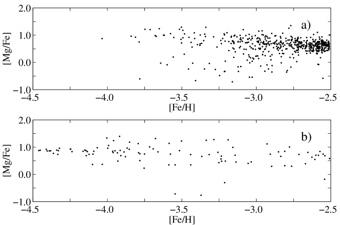
Figure 1: A sample of model stars in the [Mg$/$Fe]–[Fe$/$H] plane. Stellar yields are taken from Nomoto et al. (1997). a) Volume-limited sample of $500$ stars. b) Biased sample (see Appendix B) of $100$ stars.

The model of Argast et al. (2000) is formulated less in analytical terms than ours, i.e. it is brought to numerical form more directly. In their model the SFR scales in proportion to $\rho^{2}$, while our SFR is prescribed and, since space averages are used both for SFR and $\rho$, corresponds to a linear density dependence in this particular model. Extra-galactic infall is not explicitly considered. Also, mixing is treated differently, with a mixing-mass of $5\times 10^{4}$ M_⊙ as a standard choice for each SN which first mixes its debris into that ISM mass before any further star-formation may occur. Argast et al. (2000) also mainly explored the resulting abundances for low-mass stars for one set of yields. We shall later make some comparisons between those results and ours.

The model of Oey (2000) is physically different in that it assumes that star-formation and supernova enrichment occurs in aggregates, i.e. giant star-forming regions and superbubbles. (We note, however, that just as her model could be reformulated to the case of individual uncorrelated SNe, our model could be reformulated to the aggregated case.) Technically, her model is an elegant inhomogeneous generalization of the classical one-zone models of chemical evolution. It is closed (i.e. no extra-galactic infall) and certain uniformity assumptions must be made, concerning the filling factor of star-forming regions and the probability density function for obtaining a certain metallicity at points affected by star formation, both assumed to be the same for all stellar generations. Oey has applied her basically static model to the study of metallicity distributions for stars in the Galaxy (see also Oey 2003), but she has not explored different abundance ratios more in detail.

3 Results and discussion

3.1 Terminology and methodology

In KG we introduced the terminology “$A/$H diagrams” for plots of abundance ratios of stars like [$A/B$] vs [$C/$H], where $A$, $B$ and $C$ denote different heavy elements and H, as usual, hydrogen. The square brackets have their standard meaning, denoting logarithmic abundance ratios relative to the sun. Similarly, we denoted plots of heavy element ratios like [$A/B$] vs [$C/D$], $D$ representing another heavy element, “$A/A$ diagrams”. We shall use this terminology below.

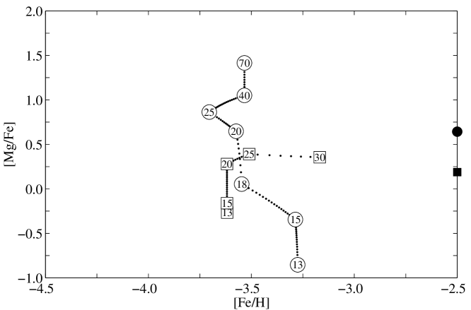
Figure 2: Stellar yields of Mg and Fe in the range $13-70\leavevmode\nobreak\ \mathcal{M_{\odot}}$ (circles) by Nomoto et al. (1997) and $13-30\leavevmode\nobreak\ \mathcal{M_{\odot}}$ (squares) by UN02. The encircled numbers denote initial stellar mass. The dots connecting the symbols are distributed according to a Salpeter IMF. The filled circle and the square at the metal-rich end mark the IMF-averaged [Mg$/$Fe] ratio given the yields by Nomoto et al. (1997) and UN02, respectively. The [Fe/H] ratio is calculated given an average mixing mass of $\overline{M}_{\mathrm{mix}}=2.25\times 10^{5}\leavevmode\nobreak\ \mathcal{M_{\odot}}$.

The synthetic $A/$H and $A/A$ diagrams will be presented both as probability density functions as well as scatter plots, where we have randomly picked a number of stars from the calculated density functions. Normally, these stars are picked with a metallicity distribution representative for the full Halo population of surviving low-mass stars, which means that the number of stars with very low metallicities is only a small fraction of the total sample. However, in many surveys of Pop II stars one does not study volume-limited samples, but deliberately aims at a biased sample, e.g. such that a roughly equal number of stars is analysed for each interval, of equal width, in logarithmic metallicity. Behind this choice may be intentions to delineate abundance trends as functions of metallicity, or a particular interest in the most metal-poor stars which requires biasing of the survey towards the discovery of those objects. In our simulations we shall show examples of both volume-limited samples of model stars, as well as samples biased towards equal number of stars for each bin in, e.g., [Fe$/$H]. The transformations from distributions of volume-limited samples to biased samples of stars is detailed in Appendix B, below.

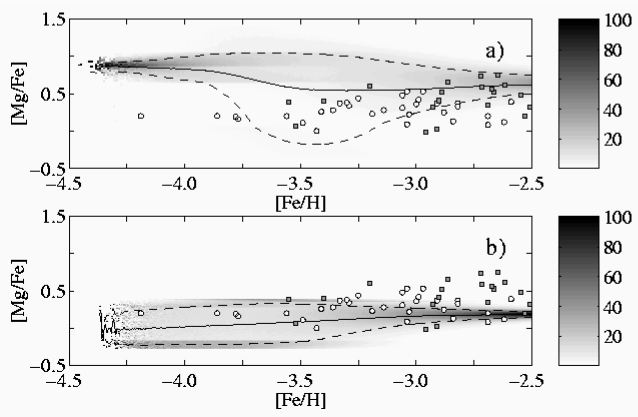
Figure 3: Probability density functions of low-mass stars in the [Mg$/$Fe]–[Fe$/$H] plane. a) The resulting density function using stellar yields by Nomoto et al. (1997). b) The corresponding function using the yields by UN02. The density functions are renormalized to a biased sample (see Appendix B) and the shaded bars indicate the relative number density of stars in arbitrary units. The full line represents the mean [Mg$/$Fe] ratio at given [Fe$/$H] and the dashed lines indicate the scatter. The small circles denote extremely metal-poor giants observed by Cayrel et al. (2004) and the gray squares denote dwarfs observed by Cohen et al. (2004).

We shall now present a number of simulated $A/$H and $A/A$ diagrams, and in passing compare them with some recent observations. We begin with a study of the $A/$H diagrams of the so-called $\alpha$ elements Mg, Si, Ca and Ti and defer a discussion of some particularities of the diagrams to the end of that study.

3.2 A/H diagrams for $\alpha$ elements

The different $\alpha$ elements Mg, Si, Ca and Ti are formed under different conditions, and their abundances thus probe different phases of the evolution of massive stars towards the supernova stage. Mg originates from the hydrostatically processed carbon core, and from explosive Ne-C burning. The amount of Mg produced (as well as of O and Ne) varies considerably with stellar initial mass, and with the extent of mixing. Si and Ca originate from explosive O- and Si-burning and their yields vary less with initial mass. They probe the progenitor model but also depend on the energy in the SN explosion and the amount of fall-back. The energy determines the excitation of the shock front passing through the model, which in turn determines the alpha-rich freeze-out from explosive Si burning, and thus the Ti yields.

(a) Mg/Fe. As a first example we show in Fig. 1a the distribution of a volume-limited sample of $500$ model stars in the [Mg$/$Fe]-[Fe$/$H] diagram. Here, we have used the SN yields of Nomoto et al. (1997), essentially the same yields as used by Argast et al. (2000). As seen when comparing to their Fig. 2, the two plots give a similar impression, which is to be expected in view of the relatively similar chemical evolution models. They both show a [Mg$/$Fe] value of $0.5$ around [Fe$/$H]$=-2.5$, with a minority population of stars with smaller Mg abundances, and an increasing scatter for [Fe$/$H] decreasing below $-3.0$. A difference is that Argast et al. (2000) find stars even more Mg-poor than our extremes, by about a factor of two. The result is, as discussed by Argast et al. (2000), not in accordance with observations, which do not disclose stars with [Mg$/$Fe] values significantly below $0.0$. We also note that the more recent surveys of abundances in stars of Extreme Pop II, Cayrel et al. (2004) and Cohen et al. (2004), do not show a single star with a negative [Mg$/$Fe] ratio. We have also used the more recent yield calculations of UN02. Their Mg yields are systematically greater, relative to those of Fe, by a factor of $3$ for the low initial masses, while they are smaller (but with Mg$/$Fe still greater than solar) for the high-mass stars (see Fig. 2). The mean value of [Mg$/$Fe] in the metal-rich end is now only $0.2$ dex, which departs from the observed value, while the most metal-poor model stars are now closer to observations although some of them still too Mg-poor.

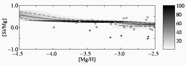
Figure 4: Probability density function of low-mass stars in the [Si$/$Mg]–[Mg$/$H] plane. Stellar yields are taken from WW95. Symbols, see Fig. 3.

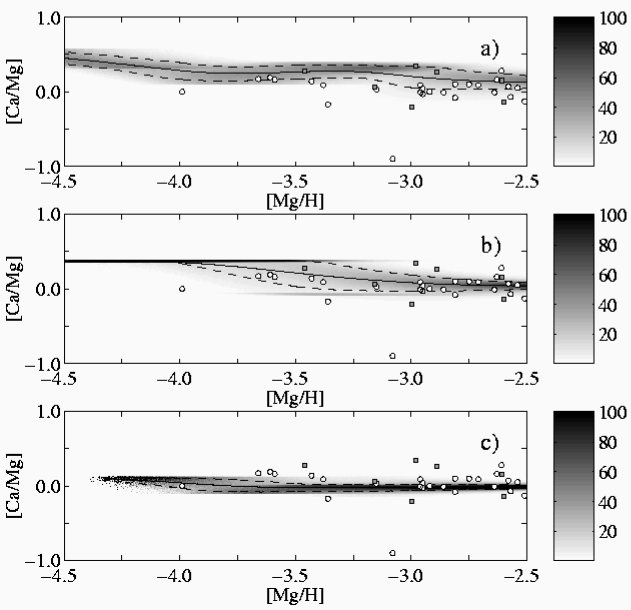
Figure 5: Probability density function of low-mass stars in the [Ca$/$Mg]–[Mg$/$H] plane. a) The resulting distribution of stars if yields from WW95 are used. b) The corresponding distribution using yields by UN02. c) Yields by CL04. Symbols, see Fig. 3.

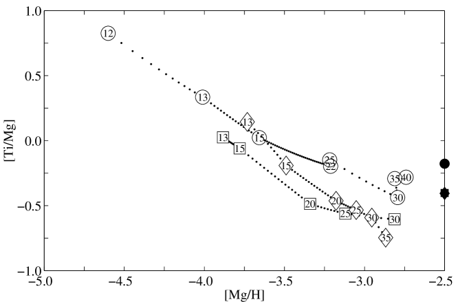
Figure 6: Three different sets of stellar yields of Ti and Mg. Yields from WW95 are indicated by circles ($12-40\leavevmode\nobreak\ \mathcal{M_{\odot}}$) while yields from UN02 are indicated by squares ($13-30\leavevmode\nobreak\ \mathcal{M_{\odot}}$) and yields from CL04 by diamonds ($13-35\leavevmode\nobreak\ \mathcal{M_{\odot}}$). Otherwise, the notation is as in Fig. 2.

In Fig. 1b we display a sample of $100$ model stars, again using the yields by Nomoto et al. (1997), biased to equal number for equal intervals in [Fe$/$H]. We note here that, unexpectedly, the scatter in [Mg$/$Fe] diminishes for the most metal-poor stars. That is, there seems to be a departure from the general law often taken for granted (e.g. by Nissen et al. 1994) and demonstrated by the simulations of Argast et al. (2000) for a number of element ratios: that the scatter should increase towards the lowest metallicities as a reflection of the small number $k$ of SNe (essentially a normal stochastic $k^{-1/2}$ dependence). Here, instead we find a diminishing scatter in the most metal-poor end of the diagram. To study the reason for this we calculated the density function in detail (cf. Appendix A), biased in equal [Fe$/$H] intervals. The resulting distribution and scatter is shown in Fig. 3a. A closer look at the yields used (Nomoto et al. 1997), shows that the lowest Fe yields are obtained for SNe with initially $25$ solar masses, and these give a [Mg$/$Fe] value of $0.8$ (see Fig. 2), as observed for the most metal-poor stars in Figs. 1b and 3a. Since the selection of contributing SNe for stars with the lowest iron abundances will be heavily biased towards those that contribute the lowest iron yields, the distribution in the diagram for the lowest metallicities will narrow down in [Mg$/$Fe]. Recall that stars with such a low metallicity were formed in the largest mixing volumes in which the yields were diluted with the largest mixing masses from the massive tail of the mixing mass distribution $f_{M_{k=1}}$, i.e., larger than $\overline{M}_{\mathrm{mix}}=2.25\times 10^{5}\leavevmode\nobreak\ \mathcal{M_{\odot}}$ which corresponds to the average mixing mass $\langle M_{\mathrm{mix}}\rangle$, as used for calculating the “standard” metallicity in, e.g., Fig. 2.

In Fig. 3b we display the analogous distribution, however calculated with the yields from UN02. Here, the situation is different, mainly because the supernova masses with the lowest Fe yields include both masses with the lowest Mg$/$Fe ratios, [Mg$/$Fe]$=-0.27$, and the slightly higher masses with much higher Mg yields, [Mg$/$Fe]$=0.28$, as shown in Fig. 2. Individual SNe of both masses may contribute to the Mg$/$Fe ratio for stars with [Fe/H] around $-4$.

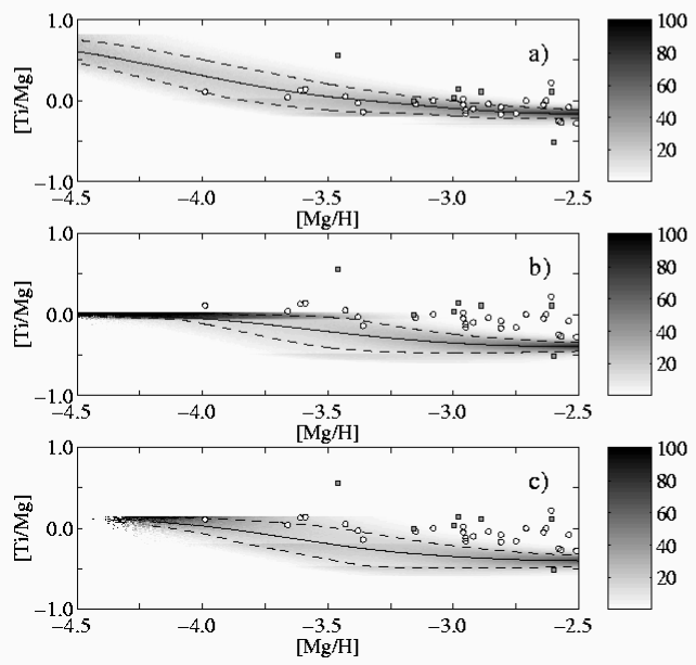
Figure 7: Probability density functions of low-mass stars in the [Ti$/$Mg]–[Mg$/$H] plane. a) Yields by WW95. b) Yields by UN02. c) Yields by CL04. Symbols, see Fig. 3.

Arnone et al. (2005) have recently explored the scatter in [Mg$/$Fe] for $23$ turn-off stars with $-3.4\leq\mathrm{[Fe}/\mathrm{H]}\leq-2.2$, and found an rms scatter of $0.06$, no larger than what is expected from uncertainties in the analysis. The different sets of yields used in this study all predict significantly greater scatter in [Mg$/$Fe] when they are applied to our inhomogeneous model. This will be commented on below.

A short comment should be made on the definition of the mean and scatter indicated by the full and dashed lines, respectively, in, e.g., Fig. 3. The mean is the usual average given by $\langle$[Mg$/$Fe]$\rangle$, at given [Fe$/$H]. The scatter is defined such that the fraction of stars outside the dashed lines is $32\%$ (at given [Fe$/$H]), $16\%$ at each side.

(b) Si/Mg. In Fig. 4 we show the density function of low-mass stars, biased to equal distribution in [Mg$/$H], in the [Si$/$Mg]–[Mg$/$H] diagram. The yields by WW95 were used here; somewhat positive [Si$/$Mg] values also show up when the yields of UN02 or CL04 are used. This moderate excess of Si relative to Mg (as compared with the solar ratio) is found observationally by Cayrel et al. (2004), while the observations for dwarfs by Cohen et al. (2004) indicate significantly lower Si$/$Mg ratios. The sloping tendency in the [Si$/$Mg]–[Mg$/$H] diagram, which may also be traced if UN02 yields are used, is not found in the observed values. The origin of the slope is the variation of the Si$/$Mg ratio with the Mg yield – the lowest SN masses, contributing least Mg and thus leading to stars in the left in the diagram, have the highest Si$/$Mg ratio, then the ratio levels off at $0.3$ dex for a range of masses (from $13\leavevmode\nobreak\ \mathcal{M_{\odot}}$ to $22\leavevmode\nobreak\ \mathcal{M_{\odot}}$) with higher Mg yields and finally drops to even lower ratios (cf. Fig. 8). A similar, though less dramatic, pattern is shown by the UN02 yields. The relatively constant level for intermediate SN masses in the WW95 yields also leads to the minimum in the dispersion in [Si$/$Mg] around [Mg$/$H]$=-3.5$ in Fig. 4.

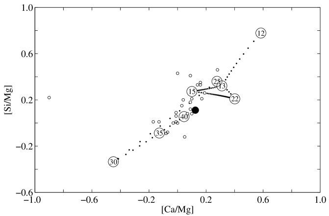
Figure 8: The yields by WW95 plotted in the $[\mathrm{Si}/\mathrm{Mg}]-[\mathrm{Ca}/\mathrm{Mg}]$ plane. The notation is as in Fig. 2. The big black dot marks the IMF-averaged point. The extremely metal-poor giants ($[\mathrm{Mg}/\mathrm{H}]<-2.50$) observed by Cayrel et al. (2004) are denoted by small circles.

(c) Ca/Mg. The scatter in [Ca$/$Mg] as a function of [Mg$/$H], displayed in Fig. 5b (i.e., UN02), shows the opposite behavior to that of [Si$/$Mg] in Fig. 4. For the dispersion in [Ca$/$Mg] there is a maximum, instead of a minimum, around [Mg$/$H]$=-3.5$. We also see a decreasing trend of [Ca$/$Mg] with increasing [Mg$/$H]. The yields by UN02 show a strong decrease of the Ca$/$Mg ratio as the Mg yields (and SN mass) increase. When WW95 yields, with a similar but more irregular behavior, are used instead, the dispersion stays more constant as a function of [Mg$/$H] while the sloping trend in the diagram still prevails. Both sets of yields, however, suggest significantly positive [Ca$/$Mg] values for the most metal-poor stars, a tendency which is found neither in the Cayrel et al. (2004), nor the Cohen et al. (2004) observed values. For the CL04 yields, the scatter stays small (reflecting a small mass-dependence of the yields), the slope only occurs for the stars with the very smallest [Mg$/$H] values, and the [Ca$/$Mg] values remain about solar, as observed.

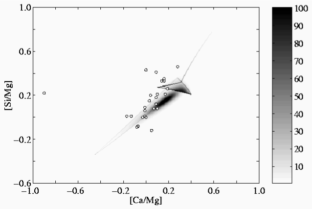
Figure 9: The full density function of stars in the $[\mathrm{Si}/\mathrm{Mg}]-[\mathrm{Ca}/\mathrm{Mg}]$ plane (cf. Fig. 8) plotted together with the observations by Cayrel et al. (2004).

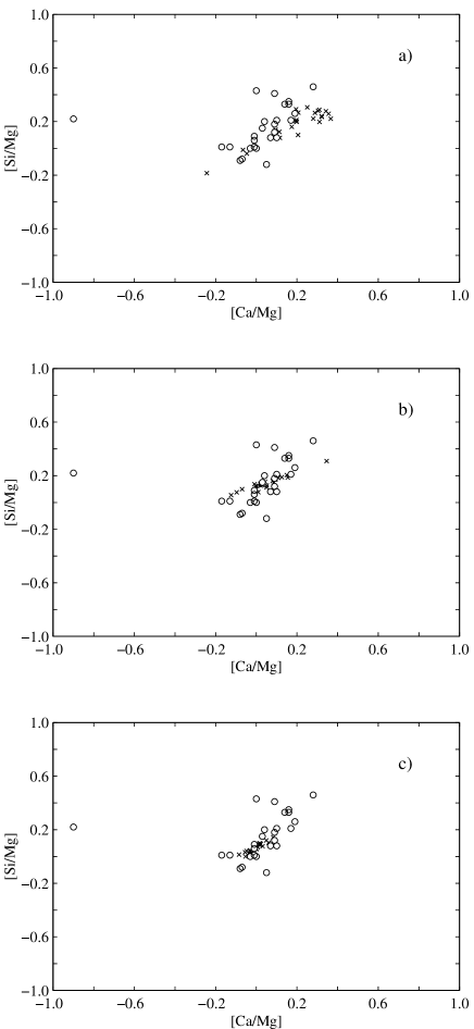
Figure 10: A sample of $25$ model stars (crosses) plotted together with the observations by Cayrel et al. (2004, small circles). a) The model stars are drawn from a density function where we used stellar yields by WW95. b) Yields by UN02. c) Yields by CL04.

(d) Ti/Mg. The relative yields of Ti$/$Mg relative to Mg for different SN initial masses are displayed in Fig. 6, for the three different sets of yields. Here, a clear negative slope in Ti$/$Mg with increasing mass, and increasing Mg yield, is seen for all three sets, although the WW95 Ti yields are systematically higher. It is easy to predict that this slope should lead to a decreasing trend in [Ti$/$Mg] with increasing [Mg$/$H], for the most metal-poor stars. The model simulations also clearly display such a trend as is seen in Fig. 7. Although, some weak trend of that character may possibly be traced in the data of Cayrel et al. (2004), as well as in Cohen et al. (2004), it is not at all as pronounced as in the simulations. We also note that the high [Ti$/$Mg] ratios predicted by the WW95 yields for the most metal-poor stars are not yet observed; obviously, the two other sets of yields on the other hand seem to give too low [Ti$/$Mg] ratios.

(e) Conclusions from the $A/$H diagrams of the $\alpha$ elements. The difference between the $A/$H diagrams calculated with different sets of yields as discussed above clearly show the possibilities of the simulations, when compared with observations of the most metal-poor stars, to illuminate the adequacy and the short-comings of different yield calculations. Within the assumptions of the model, the simulations also suggest an explanation for the astonishingly small scatter that appears in observed abundance ratios even for the most metal-poor stars. This could be the result of cosmic selection effects due to the (trivial) fact that the most metal-poor stars, formed of gas only polluted by one single SN, may predominantly originate in such clouds that are affected by SNe that produce a minimum of pollution. However, except for the unexpected small scatter in abundance ratios, there is no support for that hypothesis in the comparison with observations. The shift from one particular mass of the SNe to another one, as the metallicity increases, leads to predicted trends with metallicity that are generally not observed. Also, the narrow horizontal stripes in the left region of some $A/$H diagrams (see, e.g., Figs. 3a and 5b), mapping the effect of one dominating SN mass in the simulations, are not observed as yet.

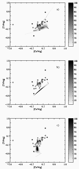
Figure 11: Distribution of low-mass stars in the [Ti$/$Mg]–[Ca$/$Mg] plane. Small circles denote the observations of extremely metal-poor giants ([Mg$/$H]$<-2.5$) by Cayrel et al. (2004), and the gray squares denote a corresponding sample ([Mg$/$H]$<-2.5$) of dwarfs by Cohen et al. (2004). a) Yields by WW95. b) Yields by UN02. c) Yields by CL04.

Several different hypotheses may be thought of as explanations for this short-coming of the model. One may be that the mixing masses are considerably larger than expected (at least a factor of ten), which will shift all the model low-mass stars towards lower metallicities. If so, we should be able to find a continuous distribution of stars down to [Fe$/$H]$<-5$ (see Paper I). Possibly, the mixing mass distributions for high numbers $k$ of contributing SNe could be significantly shifted towards higher mixing masses, e.g., due to a large increase in the infall rate of pristine gas. This will shift a number of model stars from the right (higher metallicity) side in the $A/$H diagrams to the left side (lower metallicity). Since the stellar distribution is heavily skewed towards the more metal-rich side, such a shift will lead to a considerably reduced stochastic scatter (i.e., a $k^{-1/2}$ effect). Another related possibility is that mixing with metal-free gas also occurs due to stochastic infall of intergalactic clouds. If this mechanism is to be efficient, it will require a considerable infall of clouds with masses on the order of $10^{6}\leavevmode\nobreak\ \mathcal{M_{\odot}}$ at a rate of several clouds per 1 million years, and a significant correlation between infall of these clouds and star formation; conditions that cannot be ruled out. A third interesting possibility would be that the dominating population of the most metal-poor stars in fact are Pop III stars, with originally no or very small heavy-element abundances, but polluted by gas from several SNe, accreted later, for e.g. when the stars passed through the Galactic disk (see Yoshii 1981; Yoshii et al. 1995; Shigeyama et al. 2003, see also the discussion in Christlieb et al. 2004). The small scatter in abundance ratios would then just reflect the well-mixed interstellar gas at later Galactic epochs. The possibility that this is the case is dependent on a number of uncertain conditions, such as the distribution and inhomogeneities of interstellar matter and the degree to which the stars are shielded from accretion by their own stellar winds.

Arnone et al. (2005) have recently discussed their observation that the inhomogeneous models of Argast et al. (2000) predict a far greater scatter in [Mg$/$Fe] than observed (cf. also Argast et al. 2002). In their detailed discussion, Arnone et al. (2005) suggest the possibility that shorter mixing time-scales, or longer cooling time scales than used in the inhomogeneous models could be the explanation. In the latter case, the suggestion is that longer cooling times before next generation of low-mass stars forms would admit many SNe of different masses to explode and contribute to the gas.

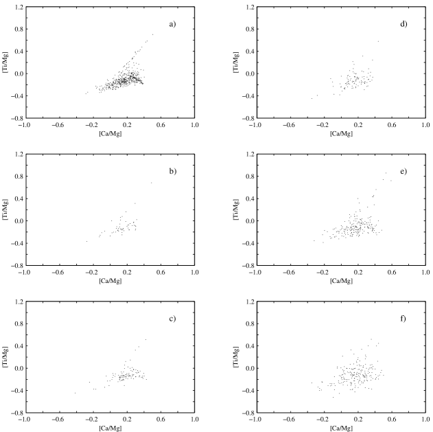
Figure 12: Model stars in the [Ti/Mg]–[Ca/Mg] plane drawn from the density function displayed in Fig. 11a. a) 500 stars with no uncertainty in the abundance ratios. b) 50 stars with no uncertainty. c) 100 stars with an uncertainty of $0.02$ dex applied in both abundance ratios. d) 100 stars with an uncertainty of $0.05$ dex. e) 200 stars with an uncertainty of $0.05$ dex. f) 200 stars with an uncertainty of $0.10$ dex.

Whatever the reason for the tendencies for mismatch between the simulated and observed $A/$H diagrams may be, we shall now proceed to $A/A$ diagrams which, as they are much less dependent on assumptions concerning mixing masses and infall of pristine gas than the $A/$H diagrams, should give more robust results.

3.3 $A/A$ diagrams for $\alpha$ elements

In Fig. 8 we have plotted the Si$/$Mg versus the Ca$/$Mg ratios of the yields of WW95 and in Fig. 9 the corresponding predicted distribution of low-mass stars. In both figures the observations by Cayrel et al. (2004) are also plotted. In general, fairly good agreement is found. We note, however, the outlier at [Ca$/$Mg]$=-0.90$ (BS 16477-003) which cannot be explained by the yields of WW95 or any of the other sets of yields discussed here. As discussed in KG, the distribution of low-mass stars in the $A/A$ diagrams is mainly determined by the stellar yields. In fact, this is illustrated by comparing Fig. 8 and Fig. 9. Visually, the two $A/A$ diagrams appear very similar and the sequence of yield ratios in Fig. 8 directly reveals the location of the “spurs” in Fig. 9 (see Sect. 3.4, below), although none of the “spurs” reaches the outlier.

Alternatively, we have in Fig. 10 plotted $25$ model stars in the [Si$/$Mg]-[Ca$/$Mg] diagram, drawn from the calculated density functions resulting from the different sets of yields (cf. Fig. 9 and Fig. 10a). For all sets, there is nice general agreement with the observations of Cayrel et al. (2004). The observations by Cohen et al. (2004) have been excluded from these diagrams. It is also noteworthy that the general trend, suggested by the models, of a positive correlation of Si and Ca excesses relative to Mg is verified by the observations, at least qualitatively. Regarding the scatter in the observations, as compared with the sequences delineated by the models, it seems that most of it may be explained as a result of observational uncertainties.

Similarly, in Fig. 11 the [Ti$/$Mg]-[Ca$/$Mg] diagrams are displayed. Here, the synthetic distributions of stars are in the form of probability density functions. There is a tendency for the models to predict somewhat low Ti abundances, as compared with the observations of dwarfs as well as of giants. The yield set of UN02 results in a narrow sequence in the diagram, with a slope close to the observed one but with an off-set by about a factor of $2$. Shifting the model stars by this off-set and introducing a Gaussian scatter of $\sigma=0.10$ in both coordinates, a reasonable estimate of the observational errors, the resulting distribution agrees well with the observed one. We may conclude that the real cosmic scatter in this diagram around the model sequence may well be very small.

3.4 The existence of “spurs” or “SSSs” in the $A/A$ diagrams

The extended narrow sequences, “spurs”, in the calculated distributions (see, e.g., Fig. 11a) represent the location of stars with major contributions from just a single supernova, though with different SN masses (see KG for more discussion as well as Idiart & Thevenin 2000 for a first, not fully convincing, attempt to trace such features). We will call these features Single Supernova Sequences (SSSs) here. An interesting issue is whether such sequences may really be traced observationally. In order to study that, we have explored the distribution of model stars, as the number of stars $N_{\star}$, as well as the random errors in [Ti$/$Mg] and [Ca$/$Mg], are varied. We use the yields of WW95. Some resulting diagrams are presented in Fig 12. From this we judge that observations of at least $200$ stars are needed for tracing an SSS, if statistical errors in the abundance observations are about $0.05$ dex (Fig. 12e) – if the errors, e.g. in a differential analysis, are reduced to $0.02$ dex the SSSs in the diagrams could appear at $N_{\star}\lesssim 100$ (cf. Fig. 12c), depending on the details in the shapes of these sequences. Contemporary differential analyses of stars of this type may possibly reach this differential accuracy (cf. Gustafsson 2004), but this is not the normal case. Also, for the purpose of finding the SSSs, it is important to have reliable estimates of the random error in the abundances, since the sharp SSSs may then be found by deconvolution. Some guidance from expectation built on theoretical yields may perhaps also be useful. It is obviously a difficult but interesting challenge to trace such features by going to large samples and accurate observations of extreme Pop II stars. If found, they will give direct evidence concerning supernova yields as well as upper IMFs for the first generation of stars. Note that a failure of finding them does not necessarily indicate that mixing between different supernova remnants have occurred before the presently observed low-mass stars formed – another possible explanation for such a failure might be the existence of another parameter besides initial mass determining the SN II yields, such as initial angular momentum.

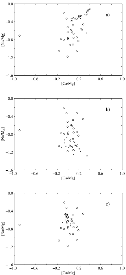
Figure 13: [Na$/$Mg] vs. [Ca$/$Mg] for a sample of $25$ model stars (crosses). Symbols, see Fig. 11. The model stars are drawn from density functions calculated using stellar yields by a) WW95, b) UN02, and c) CL04.

Figure 14: [Al$/$Mg] vs. [Ca$/$Mg] for a sample of $25$ model stars (crosses). Symbols, see Fig. 11. The model stars are drawn from density functions calculated using stellar yields by a) WW95, b) UN02, and c) CL04.

3.5 $A/A$ diagrams for Na and Al

The elements Na and Al, both with an odd number of nucleons, are sensitive to various model uncertainties in the calculation of yields. The strengths of abundance criteria for these elements are also subject to effects of departures from LTE, which are in themselves uncertain.

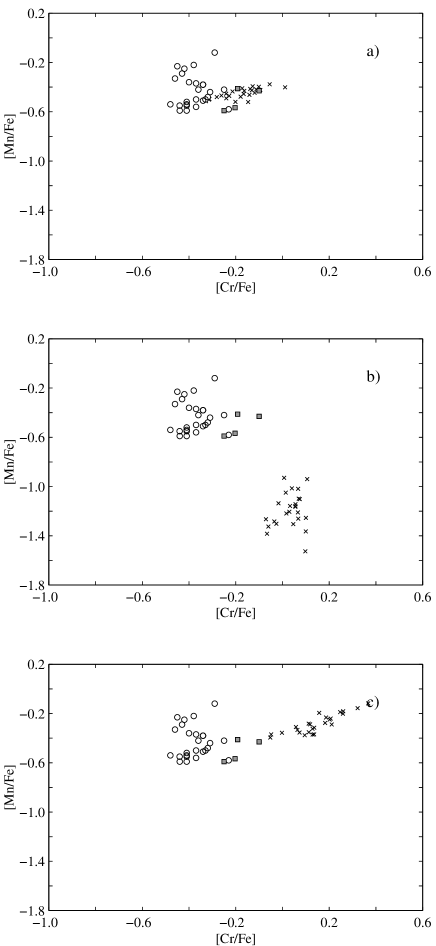
Figure 15: [Mn$/$Fe] vs. [Cr$/$Fe] for a sample of $25$ model stars (crosses). Symbols, see Fig. 11. The model stars are drawn from density functions calculated using stellar yields by a) WW95, b) UN02, and c) CL04.

In Fig. 13, we display a sample of $25$ model stars in the [Na$/$Mg]-[Ca$/$Mg] diagram, using three different sets of yields. As usual, the open circles represent observed abundance ratios of Cayrel et al. (2004), where the Na abundances are systematically corrected by $-0.5$ dex for non-LTE effects according to these authors, following Baumüller et al. (1998). It is seen that the three sets of yields depart in magnitude by as much as $0.7$ dex (such that they correspond to the observed upper level, lower level, and approximate mean level of [Na$/$Mg], respectively). The large observed scatter in [Na/Mg] is not reproduced by any of the sets of yields. We conclude that either the spurious errors in abundances (including the consideration of non-LTE effects) at least are on the order of 0.25 dex, or that the scatter in real SN yields are greater than predicted by contemporary models. A third possibility is that the abundances of some of these very metal-poor giants might be affected by hot proton burning in the ON, NeNa and MgAl cycles, as has been found for stars in globular clusters, c.f., e.g., Gratton et al. (2001). These authors find that internal mixing mechanisms in stars are not sufficient to explain the abundance effects in globular clusters but suggest mass-loss from intermediate-mass AGB stars to be active, either by contributing to lower-mass stars in slow star-forming regions (Cottrell & Da Costa 1981) or by polluting the surface layers of low-mass stars (D’Antona et al. 1983). If any of these explanations would be valid, many of the most metal poor stars must have been formed in very dense and rather long-lived star-forming regions.

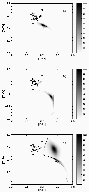
Figure 16: Density functions of low-mass stars in the [Co$/$Fe]–[Cr/Fe] plane. Symbols, see Fig. 11. a) Yields by WW95. b) Yields by UN02. c) Yields by CL04. The density function is multiplied by a factor of $5$ in order to enhance the contrast.

Some further support in this direction is obtained from the [Al$/$Mg]-[Ca$/$Mg] diagrams, Fig. 14. Here, the observed Al abundances have been adjusted upwards by $0.65$ dex to correct for non-LTE effects, according to Cayrel et al. (2004), following Baumüller $\&$ Gehren (1997) and Norris et al. (2001). We find the [Al$/$Mg] ratios as calculated from the yields to be systematically too low by $0.2-0.5$ dex, and with a predicted scatter less than the observed one.

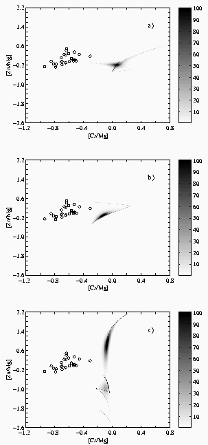
Figure 17: Density functions of low-mass stars in the [Zn$/$Mg]–[Cr/Mg] plane. Symbols, see Fig. 11. a) Yields by WW95. b) Yields by UN02. c) Yields by CL04. The density function is multiplied by a factor of $3$ in order to enhance the contrast.

We also note in passing that the recently found extremely metal-poor dwarf/subgiant star HE 1327-2326 ([Fe$/$H]$\simeq-5.4$, Frebel et al. 2005) has Na$/$Mg$/$Al ratios quite different from those of the extremely metal-poor giant HE 0107-5240 ([Fe$/$H]$\simeq-5.3$, Christlieb et al. 2004). These different results are not compatible with any of the three sets of yields explored here, and seem to support the conclusion that additional scatter of unknown origin is contributing, either from supernovae or from other sites of nucleosynthesis.

3.6 $A/A$ diagrams for the iron-group elements

In Fig. 15 we display the $A/A$ diagrams for Mn$/$Cr$/$Fe with the three different sets of yields. The synthesis of the light elements of the iron peak are usually ascribed to explosive silicon burning. It is seen that the predicted Cr$/$Fe ratios seem systematically too high by about $0.2-0.6$ dex when the model calculations are compared with the observed abundances. This discrepancy for the most metal-poor stars was also noted by Argast et al. (2000). On the other hand, the calculated Mn$/$Fe ratios turn out approximately as observed when the yields of WW95 and of CL04 are used, while they are too low by $0.8$ dex with the yields of UN02.

The $A/A$ diagrams for Co$/$Cr$/$Fe (Fig. 16) show significantly too small Co$/$Fe ratios with the yield sets of WW95 and UN02, while they come out about right for the CL04 yields. In the latter case, however, the scatter now is too large.

The Ni$/$Cr$/$Mg and Zn$/$Cr$/$Mg diagrams (see Fig. 17) are very similar and display the right order of magnitude of the Ni$/$Mg and Zn$/$Mg ratios for all sets of yields, although the CL04 yields again predict ranges which are much too large. The Cr$/$Mg ratios are too high, similar to the Cr$/$Fe ratios.

We note in general that a lower Cr yield would improve the agreement with the A/A diagrams for the iron-group elements. At least as probable as a reason for the discrepancy, however, is the presence of overionization of atomic Cr in the atmospheres of Extreme Pop II stars which would lead to systematically underestimated Cr abundances. It has earlier been proposed on observational grounds (see, e.g., François et al. 2004) that the Fe yield of WW95 is too high for their sub-solar metallicity models. A lowering of the Fe yield would increase the discrepancy in our $A/A$ diagrams even more. It is moreover not clear whether there are physical reasons to adopt such a reduction for iron only, and not for the other elements of the iron group.

3.7 A comparison with homogeneous models

Francois et al. (2004) have explored a homogeneous model of the chemical evolution of the early Galaxy, as compared with the Cayrel et al. (2004) observations. They first adopted SN II yields from WW95, although those of SN models with initial solar composition and not, as we have preferred, those with zero metallicity. The model predictions were also renormalized, sometimes by considerable amounts, to fit the abundances in the Sun. The predicted abundances give too small [Cr$/$Fe] by about $0.5$ dex as compared with the observations, which is inconsistent with our results above. For [Mn$/$Fe] Francois et al. (2004) also found somewhat low values while their predicted [Co$/$Fe] and [Zn$/$Fe] are significantly too high (by typically $0.5$ dex) for the most metal-poor stars. This is in considerable disagreement with our results, and may be explained as a consequence of the choice of initial solar abundances for the SN models as well as of the bias in their model of the most massive SNe contributing to the most metal-poor stars, as will be discussed immediately below.

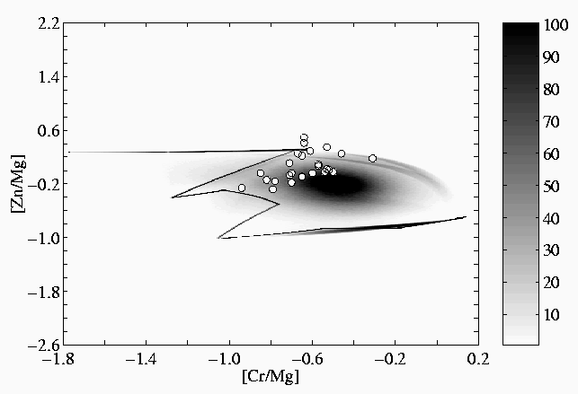
Figure 18: Density function of low-mass stars in the [Zn$/$Mg]–[Cr/Mg] plane, using the empirically determined yields by François et al. (2004). The density function is multiplied by a factor of $20$ in order to enhance the contrast. Symbols, see Fig. 11.

The trends seen at very low [Fe$/$H] in [$A/$Fe] vs. [Fe$/$H] in the François et al. (2004) results are interesting. In their model [Fe$/$H] is a direct function of time and and the relatively steep gradients in [$A/$Fe] found for certain elements $A$ reflect the gradual ”switching on” of SNe in order of decreasing initial SN mass, within the first tens of million years in the model evolution. The fact that the yields of element $A$ change when the SN mass decreases from $100$ to $10$ solar masses is thus mapped directly onto the model track in the [$A/$Fe]-[Fe$/$H] diagram. This effect cannot be obtained with our scenario, where the first stars exploding as SNe are picked randomly from the IMF, irrespectively of their lifetimes. In fact, the assumption that the most massive SNe explode first in the Galactic gas, and that they contribute their fresh elements to the gas before stars in the next mass range explode, requires mixing times in the star-forming gas of characteristically $10$ Myr or less, which seems unrealistic.

In order to improve the fit between their model tracks in the $A/$H diagrams and observations, Francois et al. (2004) have adjusted their yields as a function of SNe mass. These adjustments are considerable, in particular for elements like Mg and Cr, and drastically varying with SN mass. They would lead to strong effects for the early chemical evolution of inhomogeneous models, as seen in Fig. 18, which displays the effects in the Zn$/$Cr$/$Mg diagram with our model, however, with the Francois et al. adjusted yields (cf. Fig. 17). We note the extended spurs, mapping the very strong mass dependence of the yield ratios. This will lead to a significantly increased scatter in $A/A$ diagrams produced by inhomogeneous models, a scatter that is much greater than that observed for the first stars.

3.8 Clustered star formation

It is often argued that the generally small star-to-star scatter recently observed for many abundance ratios is a result of an averaging of the SN ejecta in a well-mixed ISM. As discussed in Sect. 3.2, a small scatter can be obtained in an inhomogeneous and poorly-mixed ISM as well (see, e.g., Fig. 5), depending on the details of the stellar yields. However, if star formation is strongly clustered, the ejecta of many SNe of different masses may mix before new stars are formed out of the enriched gas. The trends observed in several of the $A/$H diagrams would then be due to a metallicity-dependence of the IMF-averaged SN yields (“metallicity-enhancement effect”), rather than a mass-dependence of the individual SN yields (“stellar-mass effect”). A strong clustering would also wipe out the existence of SSSs in the otherwise much more robust $A/A$ diagrams.

In order to check whether clustered star formation will suppress the formation of stars enriched by a single or a few SNe to such a large extent, we randomly distributed a number of star-forming regions in a model box. Each region was given a certain size $V_{\mathrm{mix}}$, depending on the number $k_{s}$ of enriching SNe within the region. When a star-forming region overlapped with earlier formed regions, a number of model low-mass stars were allowed to form from the gas enriched by these earlier regions. This scenario is analogous to that of Oey (2000). The number of star-forming regions enriched by a certain number $k_{s}$ of SNe appears to follow a universal power-law proportional to $k_{s}^{-2}$, all the way down to $k_{s}=1$ (see Oey et al. 2004 and references therein). Assuming that this relation holds also in the young universe, we find that the number $n_{k}$ of stars enriched by $k$ SNe increases with decreasing $k$ (at least for $k\lesssim 35$), similarly to the result found in Paper I for unclustered star formation (Paper I, Fig. 5). Hence, there should presumably exist a fair number of stars only enriched by a single or a few SNe, also in an ISM with clustered star formation. In the light of this result we argue that scatter and structures, including SSSs, may be expected in the $A/A$ diagrams when observed with sufficient accuracy, independently of whether star formation is clustered or not. In Paper III, the problems of scatter related to clustering (the averaging of many SNe), cooling, and mixing of the ISM are discussed in more detail.

4 Conclusions

We have explored the predicted abundance ratios for very metal-poor stars from a stochastic model of early Galactic evolution (Paper I) for different sets of SN yields (WW95, UN02, and CL04), and compared the predictions with observations. As regards the $A/\mathrm{H}$ diagrams, we find reasonable agreement between predictions and observations for Si and Ca, although the sloping trends are in general more pronounced in the simulations (WW95 and UN02), leading to Ca/Mg ratios which are too high for the most metal-poor stars. The predicted distribution of stars also agree fairly well with observations in the [Ti/Mg]–[Mg/H] plane, however, only when the yields by WW95 are used. The presence in the simulation results, as well as in those by Argast et al. (2000), of a population of stars with very low Mg/Fe ratios are found neither in the survey of Cayrel et al. (2004), nor of Cohen et al. (2004). The small scatter in abundance ratios, also among the most metal-poor stars, may be the result of cosmic selection effects in contributing SN masses, although other phenomena may also be significant, such as different degrees of mixing of the ISM with infalling unprocessed gas, or the effects of accretion of well-mixed interstellar gas onto extremely metal-poor stars.

The distribution of stars in the more robust $A/A$ diagrams, where various abundance ratios of heavy elements are plotted relative to each other, show rather good agreement for the $\alpha$-elements Mg, Si, and Ca, as regards mean values, trends and scatter (taking observational errors into consideration). However, the yields by UN02 and CL04 produce too low Ti/Mg ratios, as is also suggested by the discrepancy between predictions and observations in the $A/\mathrm{H}$ diagrams. For the odd-even elements Na and Al, the SN yields tend to give too small abundances in general, and the predicted scatter is lower than the observed one. For the iron-group elements the calculated yields when used in our models are only moderately successful in predicting the relative abundance ratios and their scatter. The sensitivity of the appearance of the $A/A$ diagrams to the particular yields illustrates, however, the possibility of these observational data to verify, or disprove, the validity of the yields adopted.

The verification of the existence of “spurs” or “Single Supernova Sequences” in the $A/A$ diagrams, delineating stars with matter essentially affected by only one SN, is a considerable observational challenge for the future. Sample sizes of hundreds of very metal poor stars will have to be studied at very high spectroscopic accuracy and homogeneity in order to find these. However, if found they will give very valuable information about the first generation of stars and SNe. The spurs, and other structures in the diagrams, may be expected to be present, even if clustered star formation occurs instead of uncorrelated formation of single stars, as assumed in our model. If not found in future accurate surveys, it may indicate the existence of early element production by supernovae with effective mixing of the gas before any formation of low-mass stars occurred.

Appendix A Derivation of $f_{AB,CD}(x,y)$

The stochastic theory presented in KG (Karlsson & Gustafsson 2001) and in Paper I (Karlsson 2005a) is essentially built on the idea that transformations between the distribution of supernova masses and the distribution of elements in subsequently formed stars can be found, via the yields. Here, we shall present a short summary of the results given in KG. Let us first discuss the transformation between random variables in the one-dimensional case.

Let the IMF be a continuous function of stellar mass $m$ such that $\phi=\phi(m)=\phi_{0}m^{-\alpha}$, normalized as

$$\int\limits_{m_{l}}^{m_{u}}\phi(m)\mathrm{d}m=1.$$ (4)

Regarding the stellar mass as a random variable $\mathcal{M}$, the distribution of masses over the range $[m_{l},m_{u}]$ is determined by the IMF and described by the probability density function $f_{m}(m)=\phi(m)$. Similarly, the yield of an element $x=p(m)$, which we assume is a continuous function of stellar mass, will be distributed according to the random variable $X=p(\mathcal{M})$. The probability that stars generate a yield which is smaller than or equal to a certain value, i.e. $X\leq x=p(m)$, for monotonically increasing functions $p(m)$, is given by the distribution function

$$F_{X}(x) = P(X\leq x)=P(p(\mathcal{M})\leq x)$$ (5)

$$= P(\mathcal{M}\leq p^{-1}(x))=F_{m}(p^{-1}(x)).$$

The general expression for the density function (see Fig. 19) is then governed by

$$f_{X}(x) = \left|\frac{\mathrm{d}}{\mathrm{d}x}F_{X}(x)\right|=\left|\frac{\mathrm{d}}{\mathrm{d}x}F_{m}(p^{-1}(x))\right|$$ (6)

$$= \sum\limits_{i=1}^{j}f_{m}(p_{i}^{-1}(x))\left|\frac{\mathrm{d}p_{i}^{-1}}{\mathrm{d}x}\right|=\sum\limits_{i=1}^{j}\frac{\phi(p_{i}^{-1}(x))}{\left|p_{i}^{\prime}(p_{i}^{-1}(x))\right|},$$

where the yield is divided into $j$ parts such that $p=p_{1}+...+p_{j}$ and each function $p_{i}$ is monotonic and equivalent to $p$ on the open subinterval $]m_{i-1},m_{i}[$ and zero elsewhere. The $m_{i}$’s, $i=1,...,j-1$ are real roots to $p^{\prime}(m)$ and $m_{0}$, $m_{j}$ are the end-points. Similarly to the $p_{i}$’s the functions $p_{i}^{\prime}\equiv dp_{i}/dm$ on $]m_{i-1},m_{i}[$ and zero elsewhere.

Figure 19: An illustration of the transformation between random variables. The figure shows a hypothetical SN yield $p$ as a function of stellar mass (thick line). The thin vertical lines are distributed according the Salpeter IMF. The corresponding horizontal lines and the dots on the left hand side of the figure are distributed in yield-space according to the random variable $X=p(\mathcal{M})$. The probability density function of $X$, given by Eq. (6), is shown on the right hand side of the figure.

In the multi-dimensional case the transformation looks somewhat different but the idea is the same. The total ratio of two elements $A$ and $B$ produced and ejected from $k$ SNe can be regarded as a yield ratio in $k$ dimensions and is written as (cf. Eq. (26) in Paper I)

$$y^{\xi}_{k(AB)}(m_{1},...,m_{k})=\frac{\sum\limits_{i=1}^{k}\xi_{i}p_{A}(m_{i})}{\sum\limits_{i=1}^{k}\xi_{i}p_{B}(m_{i})},$$ (7)

where $p_{A}(m_{i})$ and $p_{B}(m_{i})$ are the normal one-dimensional yields for a SN of progenitor mass $m_{i}$. The weights $\xi_{i}$ on each yield is a measure of the dilution of the ejecta due to mixing with the ambient ISM and was shown in Paper I to be $\xi_{i}\equiv 1/M_{i}$, where $M_{i}$ is the mixing mass of the $i$th SN. The mixing masses are distributed according to the probability density function $f_{M_{k}}$ (see Appendix C). The weights are thus distributed according to the random variable $\Xi_{k}$, described by the density function $f_{\Xi_{k}}$. Using the result in Eq. (6), $f_{\Xi_{k}}$ is can be written as

$$f_{\Xi_{k}}=\frac{1}{\xi^{2}}f_{M_{k}(1/\xi)}.$$ (8)

Note that the distribution of mixing masses depends on $k$, the number of enriching SNe. Therefore, the weights depend on $k$ as well. As shown in KG the distributions of stars in the $A/A$ diagrams are insensitive to the distribution of the weights since probability density functions of ratios between two arbitrary, equally distributed random variables have similar shapes and are strongly peaked towards unit ratio. The presence of large-scale mixing only wipes out the structures on the smallest scales in these diagrams.

Using the definition of $y^{\xi}_{k(AB)}$ in Eq. (7), the random variable describing the total ratio between two elements is then given by

$$X^{\xi}_{k(AB)} = [y^{\xi}_{k(AB)}(\mathcal{M}_{1},...,\mathcal{M}_{k})]$$ (9)

$$= \log\left(\frac{\sum\limits_{i=1}^{k}\Xi_{k,i}p_{A}(\mathcal{M}_{i})}{\sum\limits_{i=1}^{k}\Xi_{k,i}p_{B}(\mathcal{M}_{i})}\right)-\log(A/B)_{\odot},$$

where the superscript $\xi$ is just a reminder that these functions also depend on the amount of dilution (described by $\Xi_{k}$. Recall that $\mathcal{M}$ is the random variable of stellar masses. The common astrophysical notation introduced above, where the abundance ratios are measured on a logarithmic scale relative to the Sun could as well have been introduced later as a transformation operating on the linear density functions (see Eqs. (A.16) and (A.17) in KG).

The joint distribution of the two random variables $X^{\xi}_{2k(AB)}$ and $Y^{\xi}_{2k(CD)}$ for the elements $A$, $B$, $C$, and $D$ describes how stars, enriched by $k$ SNe, would populate the [$A/B$]–[$C/D$] plane. The distribution is given by the two-dimensional function $f_{k(AB,CD)}(x,y)$, where $x=[A/B]$ and $y=[C/D]$. In its present form, Eq. (6) cannot be used to calculate multi-dimensional probability functions. Instead, we may use the alternative expression (see e.g. Papoulis 1991)

$$f_{k(AB,CD)}(x,y) = \int...\int_{\Delta D^{k}_{xy}}\phi(m_{1})\times...$$ (10)

$$\times \phi(m_{k})\mathrm{d}m_{1}...\mathrm{d}m_{k}.$$

The integrand is formed by a simple product of IMFs and does not contain any information about where the stars are distributed in yield-space. One of the main results in KG is that the chemical abundances patterns in the $A/A$ diagrams are determined by the differential integration regions $\Delta D^{k}_{xy}$. For every point $(x,y)$ in the [$A/B$]–[$C/D$] plane, $\Delta D^{k}_{xy}$ determines whether the density of stars is different from zero or not. The integrand only partly contributes to the total density. The integration region is formed by the intersection in $m$-space between $\Delta D^{k}_{x}$ and $\Delta D^{k}_{y}$, i.e., $\Delta D^{k}_{xy}=D^{k}_{x}\bigcap\Delta D^{k}_{y}$. These regions are in turn defined as

$$\left\{\begin{array}[]{ll}\Delta D^{k}_{x}=\{(m_{1},...,m_{k});\leavevmode\nobreak\ x<[y^{\xi}_{k(AB)}]\leq x+\mathrm{d}x\}\\ \Delta D^{k}_{y}=\{(m_{1},...,m_{k});\leavevmode\nobreak\ y<[y^{\xi}_{k(CD)}]\leq y+\mathrm{d}y\},\end{array}\right.$$ (11)

where the yield ratios are given by Eq. (7), although on a logarithmic scale. Thus, for any differential region in $xy$-space with a non-zero density there is at least one region in $m$-space for which the combination of masses (and dilution factors) simultaneously produces abundance ratios $x=[A/B]$ and $y=[C/D]$.

The total probability density function of ($X_{AB},Y_{CD}$), describing the distribution of low-mass stars, enriched by any number of SNe from one to $n$, is then formed by a sum of the individual density functions $f_{k(AB,CD)}(x,y)$, given by Eq. (10), such as

$$f_{AB,CD}(x,y)=\sum\limits_{k=1}^{n}w_{k}\times f_{k(AB,CD)}(x,y).$$ (12)

The normalization weight $w_{k}$ is the fraction of stars enriched by $k$ SNe such that $w_{k}=n_{k}/\sum_{k=1}^{n}n_{k}$, where $n_{k}$ is the number (kpc^-3) of stars enriched by $k$ SNe. The expression for $n_{k}$ can be found in Appendix C.

In Eq. (12), the summation is terminated at $n$, a high number of enriching SNe. However, for observational comparison, it would be more correct to let the probability density functions be terminated at a certain metallicity. Formally, this is achieved by collapsing the corresponding three-dimensional density function $f_{AB,CD,Z}(x,y,z)$ in $z$, where $z$ is the metallicity measured by, e.g., [Fe$/$H]. Analogously to the two-dimensional probability density functions described above, $f_{AB,CD,Z}$ is a sum of partial functions $f_{k(AB,CD,Z)}$ which in turn are formed by integration over the regions $\Delta D^{k}_{xyz}=\Delta D^{k}_{x}\bigcap\Delta D^{k}_{y}\bigcap\Delta D^{k}_{z}$, and where

$$\Delta D^{k}_{z}=\{(m_{1},...,m_{k});\leavevmode\nobreak\ z<[y_{k(Z)}]\leq z+\mathrm{d}z\}.$$ (13)

The expression for $y_{k(Z)}(m_{1},...,m_{k})$ is given by Eq. (26) in Paper I and describes the possible metal content (measured relative to hydrogen) of a star enriched by $k$ SNe. It is completely analogous to the expression for the abundance ratio of two heavier elements in Eq. (7). The marginal density function $f_{AB,CD}(x,y)$ is then given by

$$f_{AB,CD}(x,y)=c_{Z}\int\limits_{Z_{l}}^{Z_{u}}f_{AB,CD,Z}(x,y,z)\mathrm{d}z,$$ (14)

where $Z_{l}\rightarrow-\infty$ is the lowest possible metallicity and $Z_{u}$ is the termination metallicity (e.g. $z_{u}=[\mathrm{Fe}/\mathrm{H}]=-2.5$). the factor $c_{Z}$ is a normalization constant.

Appendix B Renormalization of $f_{AB,CD}(x,y)$

We shall briefly discuss a way of renormalizing the probability density functions for comparison with biased observational samples. Observations of stellar populations intended to map the Galactic chemical evolution are often designed such that the stars are evenly spread over the metallicity interval in log-space. However, density functions given by Eqs. (12) and (14) describe the distribution of a volume-limited sample and show an approximately exponential increase in number of stars per metallicity bin for increasing metallicity (see Fig. 6 in Paper I). Renormalization to constant density per metallicity bin is done by again integrating the three-dimensional density function $f_{AB,CD,Z}(x,y,z)$, this time with a weighting function $w(z)$ such that

$$f^{\mathrm{renorm}}_{AB,CD}(x,y) = \int\limits^{\infty}_{-\infty}w(z)f_{AB,CD,Z}(x,y,z)\mathrm{d}z$$ (15)

$$= \int\limits^{Z_{u}}_{Z_{l}}w(z)f_{AB,CD,Z}(x,y,z)\mathrm{d}z.$$

The weighting function $w(z)$ is essentially the inverse to the function $f_{Z}$, describing the distribution of stars as a function of metallicity (see Eq. (28) in Paper I) This function can also be derived from $f_{AB,CD,Z}(x,y,z)$ by collapsing the two dimensions in $x$ and $y$ such that

$$w(z)=\left(L_{Z}\int\limits^{\infty}_{-\infty}\int\limits^{\infty}_{-\infty}f_{AB,CD,Z}(x,y,z)\mathrm{d}x\mathrm{d}y\right)^{-1},$$ (16)

i.e., $w(z)$ is, except for the normalization factor $L_{Z}^{-1}=1/(Z_{u}-Z_{l})$, the inverse of the marginal density function $f_{Z}$ of $Z$. Using Eq. (16), $f^{\mathrm{renorm}}_{AB,CD}$ can then be rewritten as

$$f^{\mathrm{renorm}}_{AB,CD}(x,y) = \frac{1}{L_{Z}}\int\limits^{Z_{u}}_{Z_{l}}f_{AB,CD,Z}(x,y,z)/f_{Z}(z)\mathrm{d}z$$ (17)

$$= \frac{1}{Z_{u}-Z_{l}}\int\limits^{Z_{u}}_{Z_{l}}f_{AB,CD|Z}(x,y|z)\mathrm{d}z.$$

The function $f_{AB,CD|Z}(x,y|z)$ is the conditional probability density function of $X_{AB}$ and $Y_{CD}$ given that $Z=z$. It describes the distribution of stars in the [$A/B$]–[$C/D$] plane for a given metallicity. Integrating over metallicity will then give the renormalized density function that we seek.

Appendix C Expressions for $n_{k}$ and $f_{M_{k}}$

Assuming that the probability of finding a region enriched by $k$ SNe at time $t$ is given by Eq. (1), the total number density of stars formed in such regions in the time interval $[t,t+\mathrm{d}t]$ is $w_{\mathrm{ISM}}(k,t)\psi(t)\mathrm{d}t$, where $\psi(t)$ is the SFR per unit time and unit volume. The number of still-existing stars (enriched by $k$ SNe) per unit volume formed up to $\tau_{\mathrm{G}}$, the age of the Galaxy, is then given by the integral

$$n_{k}=\int\limits_{0}^{\tau_{\mathrm{G}}}a_{\star}(t)w_{\mathrm{ISM}}(k,t)\psi(t)\mathrm{d}t,$$ (18)

where $a_{\star}(t)$ denotes the fraction of a stellar generation formed at $t$ that still exists today and is expressed as

$$a_{\star}(t)=\int\limits_{m_{l}}^{g_{\tau}^{-1}(\tau_{\mathrm{G}}-t)}\!\!\!\!\!\!\!\!\!\phi(m)\mathrm{d}m,$$ (19)

where $\phi(m)$ denotes the normalized IMF, $m_{l}$ is the mass of the least massive stars, and $g_{\tau}^{-1}(\tau_{\mathrm{G}}-t)$ is the mass of the most massive, still-surviving stars formed at time $t$. In the early Galaxy, when most of the stars with [Fe$/$H] $<-2.5$ were formed, $a_{\star}$ changes very little. In the extremely metal-poor regime we may therefore approximate the integral in Eq. (19) with a constant such that $a_{\star}=a_{\mathrm{LMS}}$, where $a_{\mathrm{LMS}}$ is the fraction of low-mass stars with lifetimes greater than the age of the Galaxy. In Paper I, this fraction was estimated to $a_{\mathrm{LMS}}=0.835$.

Assuming homogeneous mixing, the amount of dilution of ejected SN material is proportional to the mass of the interstellar material inside the mixing volume associated with the SN. In the general case, for a time-dependent density $\rho(t)$, the total mass $M$ inside the mixing volume does not only depend on the size of $V_{\mathrm{mix}}$ but also on the time when $V_{\mathrm{mix}}$ was created by the SN explosion. Let $\tau_{V}$ be the time that has elapsed since the creation of $V_{\mathrm{mix}}$. Thus, $\tau_{V}$ denotes the age of $V_{\mathrm{mix}}$ and is a measure of its size. If the SN exploded at time $t-\tau_{V}$, the mass $M$ is given by the two-dimensional function $g_{M}$, where

$$g_{M}(t,\tau_{V})=\left\{\begin{array}[]{ll}\!\!\int\limits_{t-\tau_{V}}^{t}\!\!\!\dot{V}_{\mathrm{mix}}(t^{\prime}-t+\tau_{V})\rho(t^{\prime})\mathrm{d}t^{\prime},&t\geq\tau_{V}\\ 0,&t<\tau_{V}.\end{array}\right.$$ (20)

Note that the mass of enriched gas only grows by mixing of the surface of $V_{\mathrm{mix}}$ with the surrounding material. The mixing mass cannot change, and in particular not decrease, due to density changes within $V_{\mathrm{mix}}$. Hence, the term $V_{\mathrm{mix}}\dot{\rho}$ is excluded in the integral in Eq. (20).

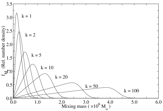
Figure 20: The distribution of mixing masses in regions enriched by $k=1,2,5,10,20,50,$ and $100$ SNe as given by Eq. (24) for a constant SFR (see Model A in Paper I).

Now, at time $t\geq\tau_{V}$, mixing volumes of size $V_{\mathrm{mix}}(\tau_{V})$ appear at a rate $u_{\mathrm{SN}}(t-\tau_{V})$, which is a measure of how many mixing volumes there are of this size at time $t$. Thus, the probability that such a mixing volume overlaps a region already enriched by $k-1$ SNe at time $t$ is proportional to $V_{\mathrm{mix}}(\tau_{V})w_{\mathrm{ISM}}(k-1,t)u_{\mathrm{SN}}(t-\tau_{V})$. The probability of forming a still-existing star in this region in the time interval $[t,t+\mathrm{d}t]$ and age interval $[\tau_{V},\tau_{V}+\mathrm{d}\tau_{V}]$ is then proportional to $a_{\mathrm{SN}}a_{\star}(t)V_{\mathrm{mix}}(\tau_{V})w_{\mathrm{ISM}}(k-1,t)\psi(t-\tau_{V})\psi(t)\mathrm{d}t\mathrm{d}\tau_{V}$, where we have assumed that $u_{\mathrm{SN}}=a_{\mathrm{SN}}\psi$. Integrating this expression over the region $\Delta D_{M}$ in the $(t,\tau_{V})$-plane gives the total probability $f_{M_{k}}$ of having a mixing mass of size $M$ in regions enriched by $k$ SNe. Thus,

$$f_{M_{k}} = c_{k}\!\!\!\!\int\limits_{\Delta D_{M}}\!\!\!\!a_{\star}(t)V_{\mathrm{mix}}(\tau_{V})w_{\mathrm{ISM}}(k-1,t)\times$$ (21)

$$\times \psi(t-\tau_{V})\psi(t)\mathrm{d}t\mathrm{d}\tau_{V},$$

where the SN fraction $a_{\mathrm{SN}}$ has been included in the normalization constant $c_{k}$. The differential integration region $\Delta D_{M}$ is defined by the function $g_{M}(t,\tau_{V})$ in Eq. (20) such that

$$\Delta D_{M}=\{(t,\tau_{V});\leavevmode\nobreak\ M<g_{M}(t,\tau_{V})\leq M+\mathrm{d}M\}.$$ (22)

Eq. (21) may be simplified by assuming that the density of the ISM is kept constant by a continuous infall of pristine gas. The mixing mass $M$ is then directly proportional to the mixing volume such that

$$M=\overline{\rho}V_{\mathrm{mix}}(\tau_{V})\equiv g_{M}(\tau_{V}),$$ (23)

where $\overline{\rho}$ is a typical density. Since the mass is determined by the size of $V_{\mathrm{mix}}$ alone, the integration over $\tau_{V}$ is redundant and Eq. (21) reduces to a one-dimensional integral

$$f_{M_{k}}=\,\,\,\tilde{c}_{k}M\!\!\!\!\!\!\!\int\limits_{g_{M}^{-1}(M)}^{\tau_{\mathrm{G}}}\!\!\!\!\!\!w_{\mathrm{ISM}}(k-1,t)\psi(t-\tau_{V})\psi(t)\mathrm{d}t,$$ (24)

where we have used Eq. (23) to write $V_{\mathrm{mix}}(\tau_{V})$ in terms of $M$, which can be taken outside the integral. The factors $a_{\mathrm{LMS}}$ and $1/\overline{\rho}$ have been included in the normalization constant $\tilde{c}_{k}$. Recall that $\tau_{\mathrm{G}}$ denotes the age of the Galaxy. Since mixing masses of size $M=g_{M}(\tau_{V})$ do not exist at times $t<\tau_{V}$, a lower integration limit is introduced at $t=\tau_{V}$, making it, as indicated, a function of $M$. Mixing mass distributions for different number $k$ of enriching SNe are plotted in Fig. 20. The derivations of $n_{k}$ and $f_{M_{k}}$ can also be found in Paper I.