Hydrodynamical simulations of the decay of high-speed molecular turbulence. II. Divergence from isothermality

Abstract

A roughly constant temperature over a wide range of densities is maintained in molecular clouds through radiative heating and cooling. An isothermal equation of state is therefore frequently employed in molecular cloud simulations. However, the dynamical processes in molecular clouds include shock waves, expansion waves, cooling induced collapse and baroclinic vorticity, all incompatible with the assumption of a purely isothermal flow. Here, we incorporate an energy equation including all the important heating and cooling rates and a simple chemical network into simulations of three-dimensional, hydrodynamic, decaying turbulence. This allows us to test the accuracy of the isothermal assumption by directly comparing a model run with the modified energy equation to an isothermal model. We compute an extreme case in which the initial turbulence is sufficiently strong to dissociate much of the gas and alter the specific heat ratio. The molecules then reform as the turbulence weakens. We track the true specific heat ratio as well as its effective value. We analyse power spectra, vorticity and shock structures, and discuss scaling laws for decaying turbulence. We derive some limitations to the isothermal approximation for simulations of the interstellar medium using simple projection techniques. Overall, even given the extreme conditions, we find that an isothermal flow provides an adequate physical and observational description of many properties. The main exceptions revealed here concern behaviour directly related to the high temperature zones behind the shock waves.

1 INTRODUCTION

State-of-the-art numerical simulations of star forming regions take into account a small selection from a wide range of relevant physical processes. Of these, it has been found that supersonic turbulent motions combined with self-gravity and magnetic field reproduce observations of the morphology and dynamics of molecular clouds on all scales (Tilley and Pudritz 2004; Bonnell et al. 2004, 2003; Padoan et al. 2004, 2003; Elmegreen and Scalo see 2004, for reviews; Mac Low and Klessen see 2004, for reviews). However, in order to reduce the computational constraints, many results are based on simulations of an isothermal gas. This implies (1) highly radiative shocks, (2) suppression of the steepening of sound waves, (3) suppression of thermal instability and shock wave overstability, (4) no adiabatic cooling in expanding regions, (5) suppression of baroclinic vorticity and (6) helicity conservation. These assumptions are not always valid and could lead to erroneous results. In addition, one can examine neither the influence of the internal properties of the gas, such as its chemical composition, on the turbulent fluid flow nor the effect of the field of shock waves on the chemical composition.

As one approach toward a more realistic scenario, we have performed numerical simulations of supersonic turbulence in dense, initially uniform, molecular material, with an equation of state determined by the chemical composition of the gas (Pavlovski et al., 2002, ; hereafter Paper I). We include a small but relevant chemical reaction network, based on the work of Smith and Rosen (2003). We follow the time-dependent hydrogen chemistry, with $\mathrm{C}$ and $\mathrm{O}$ chemistry limited to reactions with neutral atomic and molecular hydrogen, which generated $\mathrm{OH}$, $\mathrm{CO}$ and $\mathrm{H_{2}O}$ (see Smith and Rosen, 2003, Appendix B). Our cooling function contains $\mathrm{H_{2}}$ ro-vibrational and dissociative cooling, $\mathrm{CO}$ and $\mathrm{H_{2}O}$ ro-vibrational cooling, gas-grain, thermal bremsstrahlung and a steady-state approximation to atomic cooling. That is, we follow shock-enhanced chemistry rather than the chemistry of the cold molecular gas.

We demonstrated in Paper I, quite surprisingly, that even in the somewhat extreme case of high speed $\mathrm{H_{2}}$ dissociative turbulence, many integrated properties of turbulence do not differ much from the corresponding properties in the isothermal regime. In particular, the rate of loss of energy in decaying turbulence obeys a similar law. Here, we examine non-isothermal turbulence in a broader context to better understand where to trust the isothermal approximation.

Following the chemistry reveals properties not encountered in the isothermal simulations. Most importantly, we found that supersonic turbulence speeds up the reformation of hydrogen molecules by a factor of a few. This was developed by Smith et al. (2004) into a scenario for simultaneous rapid molecule and rapid molecular cloud formation out of atomic clouds. The accelerated chemistry occurs in the dense layers behind shock waves where atomic collisional rates are enhanced. After a dynamical time, the reformed molecules are widely distributed as most of the gas has at some time passed through a shock.

Here, we examine three dimensional decaying supersonic turbulence. We restrict our analysis to the high speed case of Paper I (see § 2 for description of the initial conditions; turbulence is chosen to be initially strong enough to destroy the molecules). The molecules subsequently reform and the field of shock waves then slowly decays within the molecular gas. Hereafter, we will use molecular turbulence (MT) as a shorthand for the run using the molecular chemistry network data and isothermal turbulence (IT) for the run using the isothermal equation of state.

In § 3.2, the power spectrum and cascade are analysed. Probability distribution functions (PDFs) for density, molecular density and velocity are presented in § 4. The observational implications are considered in § 5, Over the years, a number of different techniques have been proposed to interface analyses of numerical simulations with the observations (Brunt et al., 2003; Heyer and Schloerb, 1997; Ossenkopf and Mac Low, 2002; Mac Low and Ossenkopf, 2000; Padoan et al., 1998). To perform our comparison study, we apply here the same techniques to simulated observations derived from models based on both the chemical network described above and the isothermal assumption.

2 The Simulations

The gas is modelled within a three-dimensional box with periodic boundary conditions, simulated on a grid of 256³ zones using a modified version of the gas dynamics code ZEUS-3D (Stone and Norman, 1992). Paper I gives full details on the modifications to ZEUS-3D and on our initial set up.

The initial state of the gas was chosen so that we could investigate a diverse range of conditions in the subsequent evolution. The gas is initially fully molecular. The imposed velocity field corresponds to that of the highest speed turbulence from Paper I, with a root-mean-square velocity of $v_{\text{rms}}$ = (60 $\,\textup{km\,s}^{-1}$)$v_{60}$. The turbulence is allowed to decay. In this manner, we can study the initial brief period within which shocks form and molecules dissociate. This is of order of the dynamical time

$$t_{\text{dyn}}=L/(kv_{\text{rms}})=(15\,{\rm yr})L_{16}v_{60}^{-1}(k/3.5)^{-1},$$ (1)

for a box of size $L=(10^{16}$ cm)$L_{16}$ and a mean driving wavenumber $k$. This is followed by a period of molecule reformation of expected duration

$$t_{\text{ref}}=10^{10}/(nT^{1/2})\,{\rm yr}=(1060\,{\rm yr})n_{6}^{-1}T_{100}^{-1/2},$$ (2)

for a hydrogen nucleon density of $n=(10^{6}$ $\,{\rm cm}^{-3}$)$n_{6}$ and initial temperature $T=(100\mbox{ K})T_{100}$. This stage is considerably shortened by the turbulent compression. Finally, we follow an extended period of gradually decaying molecular turbulence. We set our numerical initial conditions to have $L_{16}=n_{6}=v_{60}=T_{100}=1$.

It should be noted that the total cooling length behind a fast dissociative shock at the above density is $\sim$ 10¹³ cm (Smith and Rosen, 2003) and is not resolved in the simulation, so we cannot predict quantities or instabilities inherent to the shock physics and dynamics. The corresponding cooling time is approximately

$$t_{\text{cool}}=(1\mbox{ yr})n_{6}^{-1}.$$ (3)

However, mass and momentum are still conserved, equilibrium chemistry is maintained, and the dissociation speed limits are approximately correct (Paper I). In the subsequent slower shocks within the molecular turbulence, the radiative layers are thicker and partly resolved.

The temperature in IT was fixed at 100 K. All other parameters were unchanged from the MT case. That includes the initial kinetic energy spectrum which is imposed artificially by perturbing the velocity field with a Gaussian random field following Mac Low et al. (1998). A narrow range of wavenumbers, $3<|\mathbf{k}|<4$, is chosen for the velocity perturbation.

It should be noted that the molecular simulation still excludes certain aspects of a molecular supersonic flow. The resolution precludes the appearance of the shock overstability (Smith and Rosen, 2003). The zone size limits the degree of compression although high densities can occur when material accumulates within a zone. Both these effects can only be adequately modelled by decreasing the zone size by a factor of 100 or by introducing a strong magnetic field. Equilibrium chemistry, however, allows us to proceed and to follow some of the consequences of non-isothermal shock physics.

3 POWER SPECTRA

3.1 Definitions

Power spectra of the fluid variables have long been used to characterise turbulence and so provide a standard means of comparing simulations. The total spectral power density is

$$P(k)=\sum_{k<|\mathbf{k}|<k+1}|\hat{\mathbf{v}}(\mathbf{k})|^{2},$$ (4)

where $\hat{\mathbf{v}}(\mathbf{k})=\cal{F}\left[\mathbf{v}\left(\mathbf{r}\right)\right]$ is the Fourier transform of the velocity field (and $\cal{F}$ is a Fourier operator).

According to the Helmholtz decomposition theorem, any differentiable vector field with divergence $\left(\nabla\cdot\mathbf{v}\right)$ and curl $\left[\nabla\times\mathbf{v}\right]$ can be split into compressional and solenoidal components. We thus write the velocity of the fluid as

$$\mathbf{v}\left(\mathbf{r}\right)=\mathbf{v}_{s}\left(\mathbf{r}\right)+\mathbf{v}_{c}\left(\mathbf{r}\right),$$ (5)

where

$$\left[\nabla\times\mathbf{v}_{c}\right]=0,\qquad\left(\nabla.\mathbf{v}_{s}\right)=0.$$ (6)

The solenoidal and compressional power spectra are written as

$$P_{s}(k)=\sum_{k<|\mathbf{k}|<k+1}|\hat{\mathbf{v}}_{s}(\mathbf{k})|^{2}$$ (7)

and

$$P_{c}(k)=\sum_{k<|\mathbf{k}|<k+1}|\hat{\mathbf{v}}_{c}(\mathbf{k})|^{2}.$$ (8)

The total power spectrum can also be expressed as $P(k)=P_{s}(k)+P_{c}(k)$ since $\left(\hat{\mathbf{v}}_{s}^{\ast}.\hat{\mathbf{v}}_{c}\right)=0$. Note that we consider here angle averaged quantities, which is appropriate for isotropic turbulence (by isotropic we mean that the correlation length is smaller than the computational domain; see Paper I for details).

Initially, the power spectrum of velocity also corresponds to the kinetic energy distribution (or ‘energy spectrum’) since the density is initially uniform. The initial energy is divided one-third into compressive modes and two-thirds into solenoidal modes.

3.2 Total Power Spectra

The spectral peak rapidly widens at the beginning of the simulations, as illustrated by the curves in Fig. 1 for MT (thin black line) and IT (thick grey line). It develops into a wavenumber cascade with a maximum in the same initial range $3<|\mathbf{k}|<4$ for MT. The minimum is located at the high $k$ end.

At later times, the power is redistributed into a monotonic cascade with the maximum at $k=1$ and minimum at $k=127$ (see Figs. 1). For comparison, we indicate on the diagram the power-law Kolmogorov spectrum, $k^{-11/3}$, which is expected to occur even in decaying three dimensional incompressible turbulence (Lesieur, 1997). In contrast, no clear power law develops in the spectra here as there is no continuing input of energy in the driving range in these decaying simulations and the power falls somewhat faster at high wavenumbers than at low wavenumbers in both cases (in this respect, the apparent ’convergence’ of the curves at the high $k$ end is illusory; see Table 1 for the quantitative measure of the slope angle). In terms of the spectrum of shock waves, the increasing dominance of weak shocks preferentially dissipates the energy on small scales (see § 4.4).

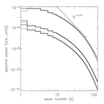
Figure 1: Evolution of the velocity power spectrum for IT case (thick grey lines) and MT (thin black lines) simulations. Data at three instances are displayed: upper lines: $t=30$ yr; medium lines: $t=300$ yr; lower lines: $t=600$ yr. See also Fig. 2.

Figure 2: Evolution of the velocity power spectrum (ratio of compressional to solenoidal energy spectra) for MT on the left and IT on the right. Data at three instances are displayed: thick lines: $t=30$ yr; thin lines: $t=300$ yr; dashed lines: $t=600$ yr. See also Fig. 1. Typical amount of variability due to the limited number statistics can be assessed from the error bars plotted for the $t=600$ yr IT case: values for large scales have smaller statistical significance as there are fewer large scale modes (the error bar for $k=1$ isn’t shown but is large since it is represented by a single value).

Time	MT	IT
$30$ yr	$-2.91\pm 0.06$	$-2.88\pm 0.06$
$300$ yr	$-3.07\pm 0.07$	$-3.07\pm 0.07$
$600$ yr	$-3.16\pm 0.07$	$-3.16\pm 0.07$

Table 1: Coefficients, $n$, of linear fits to the total energy power spectra ($\log P\propto n\log k$) for the two cases of molecular gas (MT) and gas with an isothermal equation of state (IT). The indices were measured over the interval $k\in[8,64]$ and demonstrate a systematic steepening of the curves with time.

The main result is that there is no significant difference between the evolutions of the total power spectra of MT and IT. Since the turbulence is not driven, the statistical properties of the fluid continue to change (as opposed to the dynamical equilibrium reached in driven turbulence simulations).

3.3 Compressional and Solenoidal Power Spectra

The power in compressional and solenoidal modes begins in a 1:2 ratio, as noted above. Intuitively, it might seem that the power ratio should scale with Mach number since a flow with zero Mach number is incompressible (all kinetic energy is in vortices) while a flow with a very large Mach number should be highly compressible (Elmegreen and Scalo, 2004). In our case, however, solenoidal and compressional modes are coupled and can exchange energy in both directions. Of special relevance here is how the evolution of vorticity, $\mathbf{w}\equiv[\nabla\times\mathbf{v}]$, is coupled with the divergence, $(\nabla\cdot\mathbf{v})$,

$$\begin{split}\frac{\partial\mathbf{w}}{\partial t}+\left(\mathbf{v}.\nabla\right)\mathbf{w}=&\left(\mathbf{w}.\nabla\right)\mathbf{v}-\mathbf{w}\left(\nabla.\mathbf{v}\right)\\ -&\left[\nabla\left(\frac{1}{\rho}\right)\times\nabla P\right]+\nu\nabla^{2}\mathbf{w},\end{split}$$ (9)

where $\rho$ is the mass-density of the fluid, and $P$ is pressure. The first term on the right hand side of equation (9) describes the vorticity generation due to tilting and stretching. The second term couples generation of the vorticity and divergence (if there is a negative divergence in the fluid, it will tend to shrink a fluid parcel, decreasing its moment of inertia, and, as a result, angular momentum conservation will give rise to vorticity), and the third term describes baroclinic vorticity generation. If turbulence is modelled as barotropic or isothermal, baroclinic vorticity generation is suppressed (Elmegreen and Scalo, 2004).

As displayed in Figs. 2, the ratio of compressional to solenoidal energy does not remain constant across the range of scales, with large scales being more solenoidal and small scales slightly more compressive. This is not a surprising result as compressive motions are associated with shocks which are only a few zones wide (as allowed by artificial viscosity (see, e.g., Stone and Norman, 1992)) and thin shells from subsequent radiative cooling. The shells break up due to various instabilities (Vishniac, 1983; Mac Low and Norman, 1993; Vishniac, 1994; Dgani et al., 1996).

It is remarkable that small scale compressional motions develop much faster in the MT case than in the IT case (we thank M. Bate for pointing this out). This effect can be partly due to additional thermal instabilities (Smith and Rosen, 2003) that contribute to the rapid braking of shocks in the MT case, but is more likely to be associated with the higher sound speed in the dissociated gas that allows compressive waves to steepen faster. In the IT case, large scale shocks survive longer and compressional energy gradually shifts from large to small dissipative scales. Another possibility is additional baroclinic vorticity generation in the MT case, as follows from the analysis of the equation for vorticity evolution, Eq. (9). Statistical results for shocks and vorticity will be discussed in detail in § 4.4.

Once developed, the IT becomes more compressive at high wavenumbers than MT, remaining, however, predominantly solenoidal in both cases. The inequality $P_{c}/P_{s}<1$ has also been found in a simulation of driven supersonic magnetised turbulence (Boldyrev et al., 2002; Padoan and Nordlund, 2002). Given that the total (solenoidal plus compressional) energy is the same in both simulations (see Fig. 1), we attribute this difference to baroclinic vorticity generation in MT.

A related result was also found in simulations of driven turbulence with a multiple power-law cooling function (Vázquez-Semadeni et al., 1996). The initial turbulence was purely solenoidal but was driven by purely compressible forcing. Vorticity production in this case was found to depend heavily on the additional terms (including Coriolis force on large scales, and Lorentz force on small scales).

This interplay between modes was also noted by Balsara et al. (2004). There, even though the medium is driven by highly compressible motions, the kinetic energy is mainly concentrated in solenoidal rather than the compressible motions. This behaviour was shown to arise from the interaction of strong shocks with each other and with the interstellar turbulence they self-consistently generate.

4 SIMULATED STRUCTURE

4.1 Density PDFs

The basic statistical property of a molecular cloud model or, indeed, observational data is the distribution of density. While the observational picture is essentially two dimensional, our simulations provide detailed information about the density distribution in 3D. This distribution can be described in several ways. The fractional volume distribution is

$$\text{d}{\cal P}_{V}=\Omega_{V}\text{d}\rho,\qquad\Omega_{V}=\frac{1}{V_{0}}\frac{\text{d}V}{\text{d}\rho},$$ (10)

where $\text{d}{\cal P}_{V}$ is the probability to find a value of density $\rho\in[\rho,\rho+\text{d}\rho]$ and $V_{0}$ is the total volume. Similarly, the fractional mass distribution is

$$\text{d}{\cal P}_{M}=\Omega_{M}\text{d}\rho,\qquad\Omega_{M}=\frac{1}{M_{0}}\frac{\text{d}M}{\text{d}\rho},$$ (11)

where $M_{0}=\langle\rho\rangle V_{0}$ is the total mass and $\langle\rho\rangle$ is the volume averaged density.

To describe molecular turbulence, we introduce the fractional molecular mass,

$$\text{d}{\cal P}_{\mathfrak{M}}=\Omega_{\mathfrak{M}}\text{d}\rho,\qquad\Omega_{\mathfrak{M}}=\frac{1}{\mathfrak{M}_{0}}\frac{\text{d}\mathfrak{M}}{\text{d}\rho},$$ (12)

where $\mathfrak{M}=(2/1.4)f\rho\text{d}V$ is the mass of $\mathrm{H_{2}}$ (here, $fn\times 2m(\mbox{$\mathrm{H}$})$ is the mass of $\mathrm{H_{2}}$, and $\rho=1.4nm(\mbox{$\mathrm{H}$})$ is the density of the mixture: $\mathrm{H}$, $\mathrm{H_{2}}$ and 10% of $\mathrm{He}$) and $\mathfrak{M}_{0}$ is the total mass of $\mathrm{H_{2}}$.

The distributions given by equations (10)–(12) are normalised:

$$\int_{-\infty}^{\infty}\Omega_{\Sigma}=1,\qquad\Sigma=\{V,M,\mathfrak{M}\}$$ (13)

where $\Sigma$ represents any index. Note that the $\Omega_{\Sigma}$ are not independent characteristics of the density distribution since it follows from equations (10) and (11) that

$$\Omega_{M}(\rho)=\frac{\rho}{\langle\rho\rangle}\Omega_{V}(\rho).$$ (14)

Previous analyses of $\Omega_{V}$ and $\Omega_{M}$ in simulations of compressible hydrodynamic supersonic turbulence have demonstrated that when the equation of state is approximately isothermal, the density distributions are close to log-normal, i.e. that the logarithm of density has a probability distribution function (PDF) that is a Gaussian (Vázquez-Semadeni, 1994; Padoan et al., 1997; Passot and Vázquez-Semadeni, 1998; Scalo et al., 1998; Ostriker et al., 2001). Scalo et al. (1998) found that a log-normal density PDF should only occur at (1) low Mach numbers or (2) for any value of the Mach number when the polytropic index $\gamma$ is equal to unity (i.e. in the isothermal case). Otherwise, they found density PDFs to be well approximated by power-laws over wide regions of $\log(\rho)$ variation. The simulations performed by Scalo et al. (1998) were of two-dimensional, driven, galactic turbulence, and included a variety of physical processes expected on such scales, including self-gravity, magnetic fields, rotation, heating and cooling.

It is not clear, however, whether the polytropic index (ratio of specific heats) alone is responsible for the shape of density PDFs. Li et al. (2003) studied a number of cases of turbulence with an adiabatic equation of state with different polytropic indices. In the case of driven hydrodynamical turbulence, it was found that both mass and volume PDFs show imperfect log-normal distributions. During dynamical evolution, the PDFs in the non-isothermal cases were found to develop only small deviations from Gaussian fits, while PDFs in the isothermal case ($\gamma=1$) remain very well fitted by a Gaussian. Simulations of three-dimensional, supernova-driven, galactic turbulence by Mac Low et al. (2005) also show generally Gaussian results even though heating and cooling are included explicitly, consistent with the results of Klessen (2000) who studied the PDFs of isothermal, self-gravitating turbulence. However, he found that the moments of the density PDFs vary as collapse proceeds. Hence, self-gravity is also an important factor in shaping density PDFs. It is plausible that other physical processes can affect the shape of the density PDF.

For parameterisation of PDFs with log-normal distributions, it is useful to define a dimensionless variable $\chi\,=\,\ln(\rho/\langle\rho\rangle)$. Substituting into

$$\frac{\text{d}{\cal P}_{\Sigma}}{\text{d}\rho}=\Omega_{\Sigma}(\rho)$$ (15)

yields

$${\cal P}_{\Sigma}(\chi)\frac{1}{\rho}=\Omega_{\Sigma}(\rho).$$ (16)

If $\Omega_{\Sigma}(\rho)$ is a log-normal distribution, then ${\cal P}_{\Sigma}(\chi)$ should be the normal (Gaussian) distribution

$${\cal P}_{\Sigma}(\chi)=\frac{1}{\sqrt{2\pi}\sigma_{\Sigma}}\exp\left[-\frac{(\chi-\chi_{\Sigma})^{2}}{2\sigma^{2}_{\Sigma}}\right].$$ (17)

Following the work of Li et al. (2003), we relate ${\cal P}_{M}(\chi)$ and ${\cal P}_{V}(\chi)$, using equations (16) and (14):

$${\cal P}_{M}(\chi)=e^{\chi}{\cal P}_{V}(\chi).$$ (18)

For the functional dependence given by equation (17) to be valid for both PDFs, parameters of the normal distributions have to satisfy the following relations due to Eq. (18):

$$\sigma_{V}=\sigma_{M}\equiv\sigma,$$ (19)

$$\chi_{M}=\chi_{V}+\sigma^{2},$$ (20)

$$\chi_{V}=-\frac{\sigma^{2}}{2},\quad\xrightarrow{\text{(\ref{dens:eq12})}}\quad\chi_{M}=\frac{\sigma^{2}}{2},$$ (21)

as noted by Ostriker et al. (2001).

In terms of the PDFs, the distributions $\Omega_{\mathfrak{M}}(\rho)$ and $\Omega_{V}(\rho)$ are related by

$$\Omega_{\mathfrak{M}}=\frac{f\rho}{\langle f\rho\rangle}\Omega_{V},$$ (22)

where $f$ is molecular fraction ($fn$ is abundance of $\mathrm{H_{2}}$), $\langle f\rho\rangle=(1.4/2){\mathfrak{M}}/V$. Using equations (22), (14) and (16) we can relate the normal distributions for mass and molecular mass through

$${\cal P}_{\mathfrak{M}}(\chi)=\frac{f\langle\rho\rangle}{\langle f\rho\rangle}{\cal P}_{M}(\chi).$$ (23)

4.2 The Effective Specific Heat Ratio

The actual ratio of specific heats, $\gamma$, as calculated for each zone in our MT simulation, is a monotonic function of the molecular fraction, $f$,

$$\gamma=(5.5-3f)/(3.3-f),$$ (24)

(including 10% helium). As shown in Fig. 4, $\gamma$ may vary between 5/3 and 10/7.

Figure 3: The average specific heat ratio $\langle\gamma\rangle$ employed by the code as a function of the average molecular fraction $\langle f\rangle$ in a warm molecular/atomic gas mixture (solid line); the isothermal gas case $\gamma=1$ is also shown (dashed line).

Figure 4: Long dashed line: $\langle\gamma\rangle$ the average specific heat ratio as a function of time in the MT simulation; Continuous line: $\gamma_{p}$ the effective specific heat ratio as a function of time; short dashed line: the isothermal value (1.0)

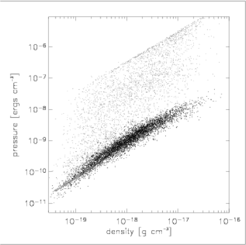
Figure 5: Scatter plots: logarithm of pressure vs logarithm of density. Grey points correspond to the time $t=10$ yr, and black points $t=600$ yr; linear fitting $\log(P)\propto\log(\rho)$ has a coefficient close to 1.0 at later times, see Fig. 4

We can define a spatially-averaged specific heat ratio by substituting $f\longrightarrow\langle f\rangle$ in Eq. (24). With these definitions, $\langle\gamma\rangle$ does not depend on the gas excitation. Hence, strictly speaking, it can serve as a good approximation only for a gas at a high temperature, to ensure that the rotational degrees of freedom are fully excited and the classical approximation for specific heats, which we employed in our model, remains valid. For molecular hydrogen, this is true for temperatures $T>85$ K. As shown in Fig. 4, $\langle\gamma\rangle$ varies considerably during the simulation.

To compare to the isothermal simulation, we define a polytropic index $\gamma_{p}$. This is the effective specific heat ratio including radiative cooling. We define it as the linear fit coefficient for the dependency

$$\log(P)=\gamma_{p}\log(\rho)+\text{const},$$ (25)

where $P$ is pressure and $\rho$ is total mass density. In Fig.5, we display the $P-\rho$ data at two times. At early times (grey cells), the dependency displays a great deal of scatter but is effectively bound between two $\gamma_{p}=1$ lines which, overall, results in the linear fitted value being close to 2, see Fig. 4. The upper line $\gamma_{p}=1$ is formed by the highest temperature regions; this temperature corresponds to $\sim$ 8000K, the post-shock temperature following rapid atomic cooling but before molecular cooling has become effective. The lower line is a reminder of the original $T=100$ K isothermal conditions. At later times (black cells in Fig. 4) the scatter is reduced, and it indicates an effective isothermality of the gas.

4.3 PDFs: analysis

In fully molecular gas $f(\rho)=\langle f\rangle=0.5$ and ${\cal P}_{\mathfrak{M}}={\cal P}_{M}$. Hence, differences between these two distributions are only going to be noticeable when strong shocks dissociate a considerable amount of $\mathrm{H_{2}}$. As shown in Fig. 4, this occurs in the first 100 yr of the simulation. Over the next 500 yr, owing to the reformation of molecules, we can expect large deviations of ${\cal P}_{\mathfrak{M}}$ from ${\cal P}_{M}$ (see also Fig. 4 of Paper I). Finally, when dissociative shocks disappear and the molecular fraction distribution flattens, ${\cal P}_{M}$ and ${\cal P}_{\mathfrak{M}}$ should converge.

The volume-weighted density PDFs in the MT run are found to be close to log-normal, as shown on the series of plots in Fig. 6 (left panel). Volume-weighted PDFs of density for Burgers’ turbulence (completely shock dominated turbulence) have been analytically shown to have power-law asymptotics (Frisch and Beck, 2001; Frisch et al., 2001). It is clear from the error bars on the plots that we can’t make a definitive statement about the asymptotic behaviour due to the lack of numerical resolution, but our results do not show clear evidence for this behavior. Numerical observations of PDF asymptotics require extremely high resolution even in one-dimensional cases (see, e.g., Gotoh and Kraichnan, 1993, 1998). We note however, that, during the early hypersonic evolution of both the IT and MT cases, the mass-weighted PDFs display clear power-law tails at low densities. We remain uncertain how to interpret this result.

To determine how much the deviation from a log-normal distribution is influenced by the high and variable value of the specific heat ratio and the introduction of explicit heating and cooling, we contrast these results with PDFs from IT (right panel of Fig. 6), which has exactly the same initial physical conditions and numerical properties. The PDFs correspond to the same moments of time. Both data sets suggest that deviations from log-normal distributions are more significant at earlier times. As turbulence decays, the distributions become more consistent with log-normal properties (see equations (19) — (21) ). We find that the PDF of density from the MT simulation is actually more consistent with a log-normal distribution than that from IT.

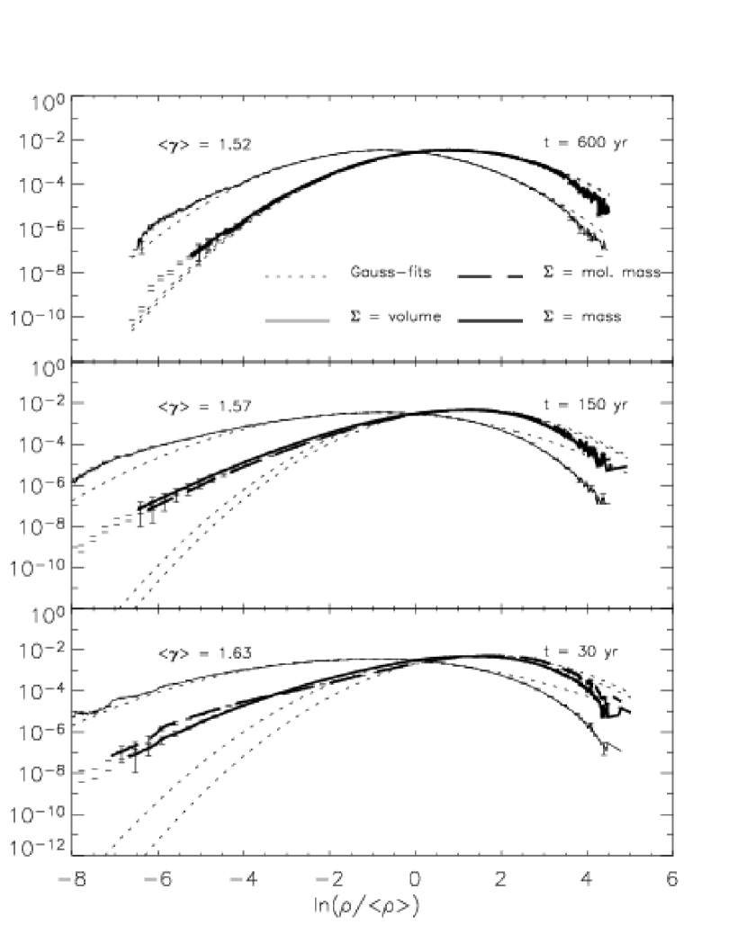
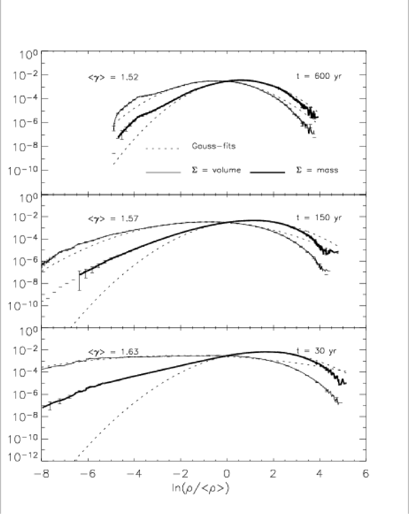
Figure 6: Evolution of PDFs of the density distribution during the simulation of decaying, high-speed, molecular turbulence including heating and cooling (MT, left panel) and isothermal turbulence (IT, right panel). Note power-law wings of the mass-weighted PDFs, and more consistent log-normal shape of the volume-weighted PDFs. To demonstrate statistical significance of the data points we plot error bars for every 20th point of each PDF curve. When statistical significance of a PDF point is small (i.e., it is derived from a single data value) the curve is traced with a small horizontal dashes (see extreme of the wings of the mass-weighted PDFs).

The evolution of the first four moments (mean $\chi_{\Sigma}$, variance $\sigma^{2}_{\Sigma}$, skewness, $\beta_{\Sigma}$, kurtosis, $g_{\Sigma}$) of the PDFs are displayed in Fig. 7. The variance, $\sigma^{2}_{V}$, exhibits a large deviation from $\sigma^{2}_{M}$ early on during both simulations. However, in the MT case the deviation is less significant. In both cases, $\sigma^{2}_{V}$ rises sharply when shocks form and distort the initially homogeneous density field. At the beginning of the simulation, in molecular gas the density contrast is less than in isothermal gas because $\gamma>1$. As shown in Fig.4, a significant hot gas phase is produced. This can qualitatively explain smaller values of $\sigma^{2}_{V}$ in a molecular turbulent flow. The variances $\sigma^{2}_{M}$ and $\sigma^{2}_{\mathfrak{M}}$ are approximately constant during the simulations. In the MT simulation, parameters of mass and molecular mass distributions converge, as expected from the above analysis.

To measure deviation of the log-distribution from gaussianity we also compute higher order moments — skewness, $\beta$, and kurtosis, $g$,

$$\beta=\frac{\mu_{3}}{\mu_{2}^{3/2}},\quad g=\frac{\mu_{4}}{\mu_{2}^{2}},$$ (26)

where

$$\mu_{n}=\langle(\chi-\langle\chi\rangle)^{n}\rangle$$ (27)

is a central moment of $n$-th order. For a normal distribution, skewness, a degree of asymmetry of the distribution, $\beta=0$, and kurtosis, a degree of peakedness of the distribution, $g=3$. For an exponential PDF the corresponding values are $\beta=2$, $g=6$. As seen from plots on Fig. 6 a significant deviation from Gaussian shape occurs only at earlier times. However, skewness remains negative throughout, indicating longer ‘tail’ on the side of low densities. It can be attributed to the fact that highest values of density are limited by the highest Mach number, whereas the lowest density does not depend on properties of individual shocks directly.

Figure 7: First moment (mean) $\chi_{\Sigma}$, second moment (variance) $\sigma^{2}_{\Sigma}$, third moment (skewness) $\beta_{\Sigma}$, and fourth moment (kurtosis) $g_{\Sigma}$ of ${\cal P}_{\Sigma}$ as a function of time in the MT (left) and IT (right) simulations. The volume mean, $\chi_{V}$ is plotted with inverse sign. A Gaussian distribution has skewness, $\beta=0.0$, and kurtosis, $g=3$, as indicated by the dotted lines.

These data suggest that $\langle\gamma\rangle$ only slightly influences the PDFs of the density distributions. Although these results are more generally applicable than specifically to large-scale, cold molecular clouds, where we would expect values of polytropic index $\gamma\approx 1$, it is remarkable that an entirely different equation of state leads to qualitatively and quantitatively very similar statistical properties.

4.4 Velocity: vorticity and shock fields

As remarked above, the assumption of isothermal or isentropic flow stops baroclinic vorticity creation. It also forces helicity, $\omega=\langle(\mathbf{v}\cdot\mathbf{w})\rangle$, to be conserved in an unphysical way in general compressible flows. In this sub-section, we analyse in detail the differences in the amount of vorticity and shocks in the MT and IT cases.

The vorticity distribution is displayed in Fig. 8. In isotropic, incompressible, turbulent flow, high vorticity exists in thin coherent tubes, as found in direct numerical simulations (DNS) with high resolution (see, e.g., Lesieur et al., 2003; Titon and Cadot, 2003). The vorticity tubes have a diameter of a few Kolmogorov dissipative scales and a length of the order of the integral scale (i.e. the driving scale). Centres of the vorticity tubes form one dimensional filament-like structures that are the centres of energy dissipation of the flow.

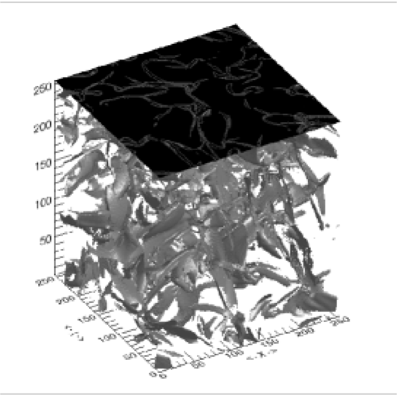
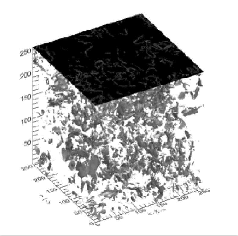
Figure 8: Left cube: Surfaces of isovorticity, $\big{|}[\nabla\times\mathbf{v}\big{|}=\text{const}$ at 10 yr after the start of the MT simulation. Shocks have just formed and large structures are present. The black upper face of the cube contains a contour plot of the top slice of vorticity. Right cube: surfaces of isovorticity at the later time of 300 yr when the shocks have fragmented.

In compressible flow, on the other hand, vorticity structures form sheets and spirals (Porter et al., 2002). In our simulations of decaying supersonic turbulence, we find that the vortex structures (isosurfaces of high vorticity) form “open” surfaces. The size of these surfaces is closely correlated with the size of shock surfaces (Fig. 9). Isosurfaces of strong vorticity become smaller with time, with a characteristic size of order of the shock size, as displayed in Figs. 8 and 9.

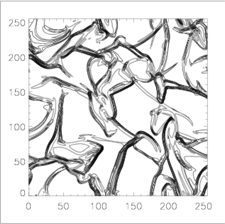
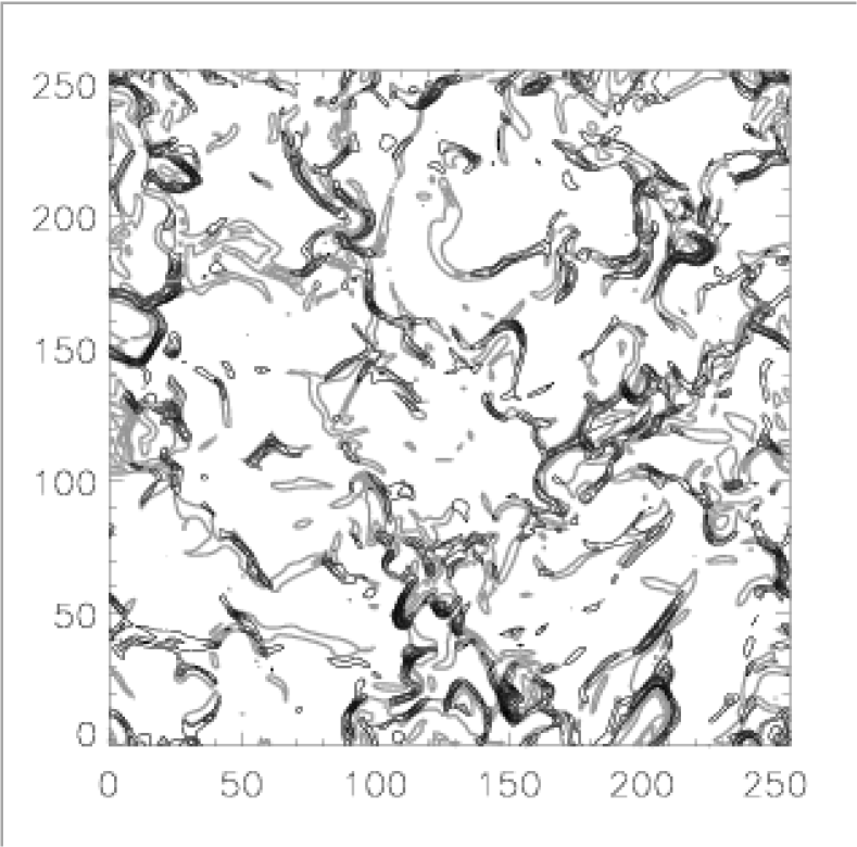
Figure 9: Contour plots from the MT case of negative velocity divergence (black) and contours of the vorticity field (grey). Note that the vorticity is concentrated around the shocks. The plots display random slices from the data cubes at $t=10$ yr (left) and $t=300$ yr (right).

Statistical analysis of the vortex structures reveals that vorticity components as well as velocity gradients have PDFs of exponential type, i.e., proportional to $\exp\{-|X|\}$, in incompressible turbulent flow. This is instead of the Gaussian distributions proportional to $\exp\{-|X|^{2}\}$ that would be expected for statistically independent structures due to the Central Limit Theorem. In laboratory experiments and DNS, regions of high vorticity correlate with regions of low pressure (Lesieur, 1997, p.196). The exponential form of the PDF of vorticity is a manifestation of the intermittency of energy dissipation. If dissipative structures were distributed homogeneously, the PDF would be given by a Dirac delta function, or a narrow Gaussian distribution in a DNS. Therefore, a deviation of the PDF of dissipative structures from the Gaussian shape is a direct indication of the intermittency of turbulence.

To study PDFs of shock waves we define the function of convergence, $\text{conv}(v)$,

$$\text{conv}(v)=\begin{cases}\left(\nabla\cdot\mathbf{v}\right),&\text{when}\left(\nabla\cdot\mathbf{v}\right)<0,\\ 0,&\text{otherwise}.\end{cases}$$ (28)

A simple statistical analysis of the converging regions and vorticity reveals the expected exponential PDFs for both fields (Fig. 10). Exponential laws for PDFs related to convergence were reported before by Smith et al. (2000b), where the distribution of shock jump velocities in a single direction were found to be approximated by an exponential:

$$\begin{split}\text{d}N&\equiv\bigg{[}\text{number of zones with }\Delta v_{i}\in[\Delta v_{i},\Delta v_{i}+\epsilon]\bigg{]}\\ &\propto\exp\{-C\Delta v_{i}\},\end{split}$$ (29)

where $C$ is a positive constant, and $\epsilon$ is a small discretisation parameter.

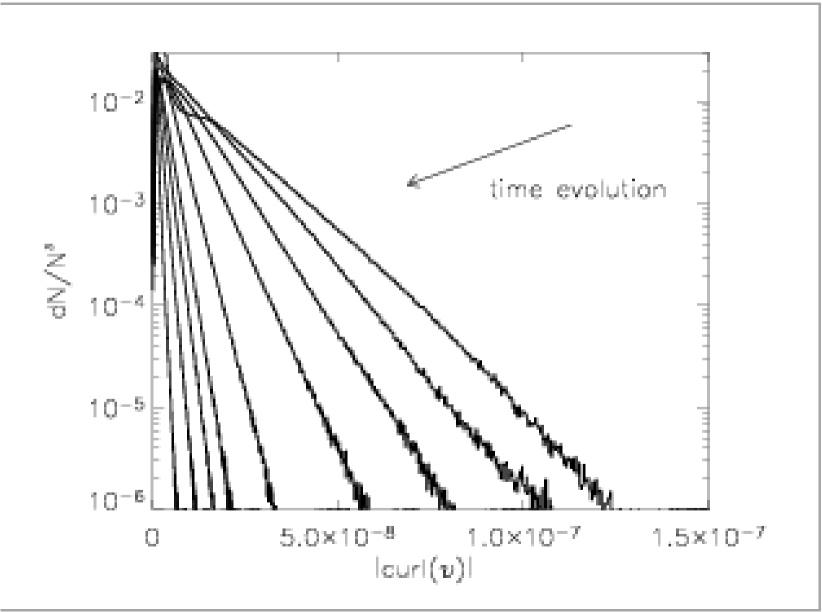
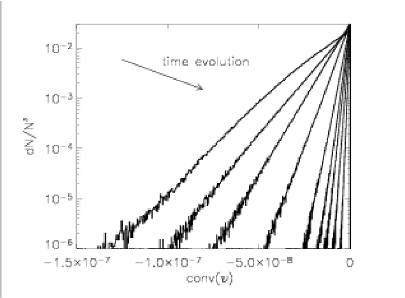
Figure 10: Left panel: histograms of $\big{|}\text{curl}(v)\big{|}$ at different times (MT simulation). Right panel: histograms of $\text{conv}(v)$ at different times (MT simulation). The histograms correspond to the following simulation times: 10, 20, 30, 50, 100, 150, 200, 300, 600 [yr], with the direction of the time sequence marked by the arrows on the figures i.e. the distributions steepen.

We find that the PDF of $\text{conv}(v)$, which is essentially a 3D generalisation of Smith et al.’s one dimensional jump velocity, has the same exponential dependence,

$$\frac{\text{d}N}{N^{3}}\propto\exp\{-\beta|\text{conv}(v)|\},$$ (30)

where $\text{d}N$ is the number of zones with $\text{conv}(v)\in[\text{conv}(v),\text{conv}(v)+\epsilon]$ and $N^{3}$ is the total number of zones (see Fig. 10). We have chosen the discretisation parameter $\epsilon$ to create $500$ bins for our histograms.

Vorticity PDFs are studied using the modulus of curl, $\big{|}\text{curl}(v)\big{|}\equiv\big{|}[\nabla\times\mathbf{v}]\big{|}$. We find that the PDF of curl behaves very similarly to the PDF of convergence but with different parameters:

$$\frac{\text{d}N}{N^{3}}\propto\exp\{-\alpha|\text{curl}(v)|\}.$$ (31)

The coefficients $\alpha$ and $\beta$ change as the turbulence decays. Both PDFs become progressively steeper with time, indicating that strong shocks and vorticity disappear. However, we find that the PDFs of convergence and vorticity do not change with time if we compensate for the average convergence and curl decay. The coefficients $\alpha$ and $\beta$ of the distributions,

$$\frac{\text{d}N}{N^{3}}\propto\exp\{\alpha\frac{|\text{curl}(v)|}{\langle|\text{curl}(v)|\rangle}\},$$ (32)

$$\frac{\text{d}N}{N^{3}}\propto\exp\{\beta\frac{\text{conv}(v)}{\langle\text{conv}(v)\rangle}\},$$ (33)

do not significantly change during the simulation. The values of the coefficients for MT and IT simulations are given in Table 2. These values may be significant constants characterising decaying turbulence.

	MT	IT
$\alpha$	$2.63\pm 0.05$	$2.61\pm 0.06$
$\beta$	$2.48\pm 0.05$	$2.30\pm 0.05$

Table 2: Coefficients of compensated PDFs of convergence ($\beta$) and module of curl ($\alpha$). The error estimates are derived from the statistical variance of the distributions of the coefficients derived from different moments in time).

The data in Table 2 suggest that the compensated PDF of vorticity is not influenced strongly by a different equation of state, whereas the compensated PDF of convergence is steeper in the MT case. A shallower PDF of convergence implies the existence of larger quantities of strong shocks in the IT case, which is not surprising. Shock jump conditions imply that in the case when the ratio of specific heats $\gamma>1$, the velocity difference across zones of the shock is smaller than in the case when $\gamma=1$. This may qualitatively explain the steeper PDF of convergence in molecular turbulence.

The PDF of the velocity itself is not very well understood (Elmegreen and Scalo, 2004). The usual argument is that the velocity PDF should be Gaussian is based on the central-limit theorem applied to Fourier components of the velocity field. This argument, however, does not take into account correlations which are important for energy transfer among scales. In fact, the velocity PDF must possess non-zero skewness for the transfer to be possible (see, e.g., Lesieur, 1997).

Analytical studies of Burgers’ (shock-dominated) turbulence found that the gradient of the velocity has power law asymptotics (same as density, see Frisch and Beck (2001)). We do not see this effect in our simulations, perhaps because of our limited numerical resolution (see also §4.3).

In our simulations, the initial distribution of the velocities has imposed Gaussian statistics. We find that deviations from the Gaussian distribution do occur but they are minor. To illustrate this, in Fig. 11 we plot the PDFs of the velocity magnitude, $v=\sqrt{x^{2}+y^{2}+z^{2}}$, which takes the form of a Maxwell distribution, i.e. $\exp\{-Av^{2}\}v^{2}$, as expected.

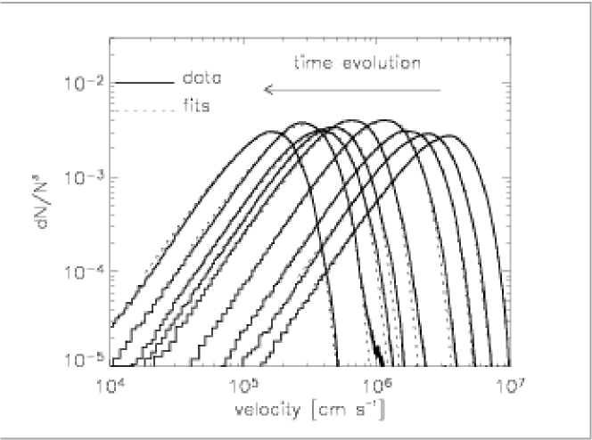
Figure 11: PDFs of the velocity magnitude during the MT simulation. The peak shifts toward smaller values as the turbulence decays. Plotted curves correspond to the same moments of time as curves on Figs. 9 & 10. The arrow points in the direction of time (velocities decrease). Dotted lines show Maxwellian fits.

5 SIMULATED OBSERVATIONS

5.1 Background

Observational predictions from numerical results have generally involved the post-processing of isothermal flows to generate simulated observations (Falgarone et al., 1994; Padoan et al., 1998; Lazarian et al., 2001; Ossenkopf and Mac Low, 2002; Brunt et al., 2003). We can validate such an approach by comparing synthetic maps from isothermal models to similar maps from the molecular models. We note that the compact and dense regime taken in our simulations is not directly comparable to existing observations of molecular clouds but rather corresponds to dense cores.

Interstellar clouds appear to follow a scaling relation first inferred from an analysis of observational data by Larson (1981). Larson used $\mathrm{{}^{13}CO}$ (optically thin line) maps of different molecular clouds to establish a size–linewidth relation

$$\sigma_{v}\propto\lambda^{b},\quad b=0.5\pm 0.2,$$ (34)

where $\sigma_{v}$ is the velocity dispersion and $\lambda$ is the size of the region.

A theoretical explanation for this scaling relation can be inferred from the following argument. The velocity dispersion, $\sigma_{v}$, can be approximated by the square root of the second order velocity structure function,

$$S_{2}=\langle\left(\mathbf{v}(\mathbf{r})-\mathbf{v}(\mathbf{r}^{\prime})\right)^{2}\rangle\propto\lambda^{\zeta_{2}},\quad\lambda\equiv|\mathbf{r}-\mathbf{r}^{\prime}|.$$ (35)

The value of $\zeta_{2}$ is determined from the model of driven supersonic turbulence proposed by Boldyrev (2002), based on the dimensionality of the dissipative structures. Boldyrev’s theory suggests the following scaling law:

$$\sigma_{v}=\lambda^{0.37},$$ (36)

which is in good agreement with the above cited observational value. Pure K41 scaling gives smaller values of the exponent ($b\approx 0.33$). However, in the case of decaying turbulence Boldyrev’s scaling laws do not apply. As we have demonstrated in Section 3, decaying turbulence results in a shallower power law energy spectrum than follows from K41 theory. To estimate the exponent $b$ in this case we can use the connection between velocity and power spectrum statistics,

$$P_{1}(k)\propto k^{-m},$$ (37)

$$S_{2}\propto\lambda^{m-1},$$ (38)

where $P_{1}(k)$ is the (one dimensional) power spectrum; using the notation of section 3, $n=m+2$ (see, e.g., Frisch, 1995). Using values of $n$ given in Table 1, $m\approx-0.88\ldots-1.16$, which implies, $b=-0.06\ldots 0.08$. Hence, we can predict that $\sigma_{v}$ should not exhibit strong scaling in the case of decaying turbulence.

Deduction of Larson’s scaling law from the observations is not a straightforward task. The width of a spectral line, broadened by the turbulent motions, is essentially the width of a composite line, contaminated by all the gas motions along the line of sight. How the width of such a composite line should depend on the size of the sampled region is not obvious. If we sample $\sigma_{v}$ from the regions that appear to be cores (i.e. continuous prominent patches of radiation intensity), sorting the $\sigma_{v}$ measurement by the size of such cores, we might stand a better chance of recovering true velocity scaling. This is because such cores may actually be coherent 3D structures, although there is no way we can protect our statistics from unavoidable mistakes (Vázquez-Semadeni et al., 1997; Pichardo et al., 2000; Ballesteros-Paredes and Mac Low, 2002). We have no means of distinguishing between “false” cores — column density enhancements produced by overlapping, unrelated density enhancements assembled by chance along the line of sight — and true cores — compact 3D objects. In regions of active star formation where self-gravity effects are important, we can hope that the number of such mis-identifications will be effectively minimised.

In the case we are studying, there is no boosting of contrast due to self-gravity but there are additional contrast parameters: the chemical composition and temperature distributions. Indeed, our simulations provide detailed pictures of the $\mathrm{H_{2}}$ and temperature distributions. Non-uniform chemical tracers may provide additional contrasts to the maps. What sort of regions can chemical tracers emphasise? As we found out in Paper I, the distribution of molecules in decaying turbulence is rather homogeneous, and there is no evidence that the $\mathrm{H_{2}}$ distribution alone will highlight 3D structures within the simulated region. However, the contrast in temperatures is far more distinct. Most of the gas in the simulated domain stays cool due to the efficient cooling; only sufficiently strong shocks can temporarily heat up the gas in certain regions, up to several thousand degrees. Hence, if we select a tracer sensitive to the temperature, we would be able to construct maps of regions with different values of temperature.

Temperature sensitive tracer maps may help answer another question relevant to the present study. Is detailed information about molecule and temperature distributions crucial for predicting emission, or is the zero-order approximation of isothermality sufficient?

5.2 Scaled projection of CO emission

The gas in our simulation is relatively warm with an average temperature $\gtrsim 100$ K (Fig. 12). Rotational emission lines of $\mathrm{{}^{12}CO}$ are a suitable tracer in this temperature range (McKee et al., 1982). Emission from the transitions between states with different rotational quantum number $J$ (only $J\rightarrow J-1$ transitions are allowed due to the quantum selection rule) will highlight regions with different temperatures. The choice of this particular tracer is reasonable because our molecular code actually computes the equilibrium abundance of $\mathrm{CO}$ to account for the cooling through rotational and vibrational $\mathrm{CO}$ emission.

Figure 12: Histogram of the temperature distribution at $t=60$ yr. The histogram has $1000$ bins with size $\delta T=16$ K. A large fraction of the gas has temperature close to $T=100$ K. The average temperature is $\approx 630$ K. Data taken from the MT simulation.

We take the non-LTE formulae presented by McKee et al. (1982). We assume that each emission line is optically thin and, therefore, the intensity of the emission (the “brightness” of the pixel on the emission map) is proportional to the column density of $\mathrm{CO}$,

$$\text{emission at $J$ level }\propto\sum\langle n_{J}(\mbox{$\mathrm{CO}$})\rangle_{i}\Delta h_{i}$$ (39)

where $\langle n_{J}(\mbox{$\mathrm{CO}$})\rangle_{i}$ is the average number density of $\mathrm{CO}$ at level $J$ in the cell of size $(\Delta h_{i})^{3}$.

The simplest way to construct a synthetic map of $\mathrm{CO}$ emission is to map the column density, as prescribed by equation (39). Following the work of Ostriker et al. (2001), we identify a clump as a region of contrast (ROC), which is regarded as such if its $\mathrm{CO}$ column density is at least a factor of $c_{r}$ larger than the mean column density of $\mathrm{CO}$ for the entire map. This procedure is somewhat similar to the procedure of subtracting “background” in the reduction of observational data. In our current study, we fix $c_{r}=1$, i.e. all regions with column density larger than the mean column density are identified as ROCs, and we constrain our analysis to the data we infer from the ROCs only.

To deduce the relationship between line width and size from the synthetic maps, we need an algorithm for the detection of ROCs of different sizes. One means of achieving this is by constructing “blurred” maps of lower resolution by rescaling the original map of $\mathrm{CO}$ column density by a certain factor, as proposed by Ostriker et al. (2001). We rescale the original $256^{2}$ grid by a factor of $2^{s}$, where $s=0,1,2,\ldots,7$. This results in eight maps with resolutions $2^{2},\,4^{2},\,8^{2},\ldots,\,256^{2}$, which we can employ for ROC identification.

To construct $\mathrm{CO}$ emission maps from the IT simulation with $T=100$ K we need to determine an appropriate abundance of $\mathrm{CO}$ (in each computational zone) without having information about the $\mathrm{H_{2}}$ abundance. The chemistry algorithm implemented in our version of ZEUS-3D implies that, for this temperature all free gas-phase carbon is in the form of $\mathrm{CO}$ for all plausible mass densities and $\mathrm{H_{2}}$ fractions. The total abundance of $\mathrm{C}$ is fixed in the code, $\mathfrak{f}(\mbox{$\mathrm{C}$})=2.0\times 10^{-4}$. Hence, in the isothermal case we take the distribution of $\mathrm{CO}$ as homogeneous with the fixed value of $2.0\times 10^{-4}$.

We select the time when the largest fraction of the molecular gas is at $T=100$ K (see the temperature histogram in Fig. 12). The actual shapes of lines and maxima in $\mathrm{CO}$ emission will depend on the underlying mass density distribution and velocity along the line of sight.

To be able to compare the morphological features directly we use density and velocity data from the MT simulation in both cases. The actual distributions of $\mathrm{CO}$ and temperature are employed for the MT maps, and homogeneous distributions of $\mathrm{CO}$ and temperature for the IT maps. We will refer to such isothermal data as quasi-isothermal. As we will show, the results of the analysis of the quasi-isothermal maps are very similar to the results of the analysis with the actual isothermal simulation data. This is not surprising giving that the statistical properties of the density and velocity fields in both simulations are very similar, as established in §§ 4.4 and 4.1.

For each ROC, we compute the mass-weighted dispersion of the line-of-sight velocity $\sigma_{v}$, which represents the line width for a region of projected area $[(L/N)/2^{s}]^{2}$. We record $M(\mbox{$\mathrm{CO_{J}}$})$ within each ROC, and the virial parameter,

$$\alpha=\frac{5\sigma_{v}^{2}[(L/N)/2^{s}]}{GM(\mbox{$\mathrm{CO_{J}}$})},$$ (40)

where $M(\mbox{$\mathrm{CO_{J}}$})$ is the mass of the $\mathrm{CO_{J}}$ ($\mathrm{CO}$ responsible for $J\rightarrow J-1$ emission) and $G$ is Newton’s gravitational constant (Ostriker et al., 2001). The parameter $\alpha$ is directly proportional to the ratio of kinetic energy to gravitational energy, and represents a measure of the relative importance of gravity (McKee and Zweibel, 1992; Ostriker et al., 2001).

5.3 Analysis of the emission maps

We now present the results of the synthetic observations. For the data sets discussed in section 5.2, we have constructed $\mathrm{CO}$ (4–3) emission maps that highlight the gas at temperatures around $100$ K (for gas with average density of $10^{6}$$\,{\rm cm}^{-3}$), and $\mathrm{CO}$ (20–19), which traces much hotter gas of about $1000$ K (McKee et al., 1982).

$\mathrm{CO}$ (4–3) emission maps for the MT data and the quasi-isothermal data are presented in Fig. 13. The similarity of these maps is quite remarkable. Differences are difficult to detect. This supports the claim made in Paper I that isothermal simulations are suitable for mapping molecular emission.

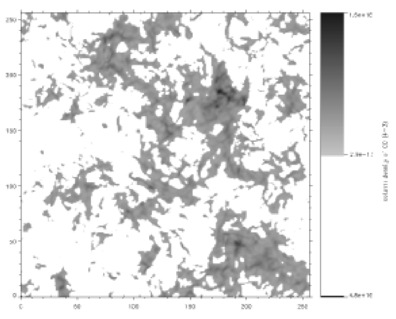
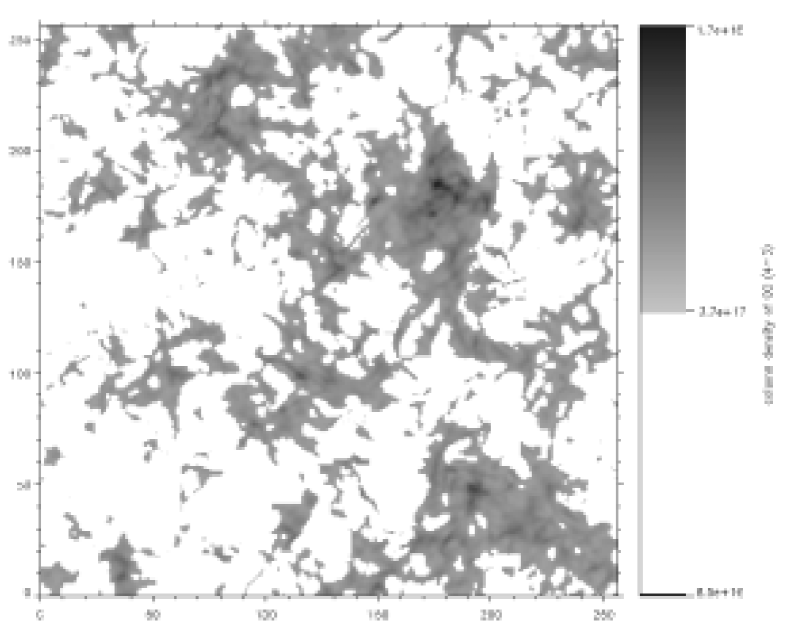
Figure 13: Maps of $\mathrm{{}^{12}CO}$ $J=4\rightarrow 3$ emission constructed from the MT data (upper panel), and the same emission map constructed from the quasi-isothermal turbulence data (lower panel), as described in section 5.2.

An analysis of the statistical properties of these maps also reveals no significant discrepancies. In Figs. 17–17, we display scatter plots of the parameters of the ROCs which were identified on the MT maps at eight different resolutions. Each point or small dash on the plots corresponds to the parameters of a ROC. Although there is a general trend in mean dependences, there is plenty of scatter in all the plots. The solid lines represent least-square linear fits of the form

$$\frac{\text{d}\log\sigma_{v}(\lambda)}{\text{d}\log\lambda}=b,$$ (41)

where $\lambda=(L/N)/2^{s}$ is the size of the ROC;

$$\frac{\text{d}\log\sigma_{v}(\lambda)}{\text{d}\log M_{\lambda}(\mbox{$\mathrm{CO_{J}}$})}=b^{\prime};$$ (42)

$$\frac{\text{d}\log\alpha}{\text{d}\log M_{\lambda}(\mbox{$\mathrm{CO_{J}}$})}=c;$$ (43)

$$\frac{\text{d}\log M_{\lambda}(\mbox{$\mathrm{CO_{J}}$})}{\text{d}\log\lambda}=d.$$ (44)

The parallel dashed lines in the figures mark the $1\sigma$ deviations for the fits. The values (41) – (44) deduced from the MT data are as follows,

$$\begin{split}b&=(2.6\pm 0.4)\times 10^{-2},\quad b^{\prime}=(1.7\pm 0.2)\times 10^{-2},\\ c&=-(4.94\pm 0.04)\times 10^{-1},\quad d=1.984\pm 0.003.\end{split}$$ (45)

The values $b$, $b^{\prime}$, $c$ and $d$ deduced from the map constructed from the quasi-isothermal data are the same within the error estimates:

$$\begin{split}b&=(2.7\pm 0.4)\times 10^{-2},\quad b^{\prime}=(1.7\pm 0.2)\times 10^{-2},\\ c&=-(4.86\pm 0.04)\times 10^{-1},\quad d=1.985\pm 0.003.\end{split}$$ (46)

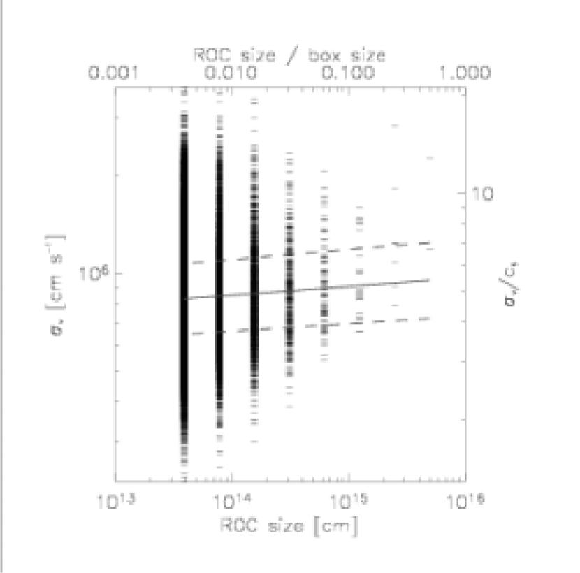
Figure 14: Sigma vs. size of ROC for the $J=4\rightarrow 3$ molecular turbulence map. For reference, $c_{s}$ is the mass-weighted average speed of sound.

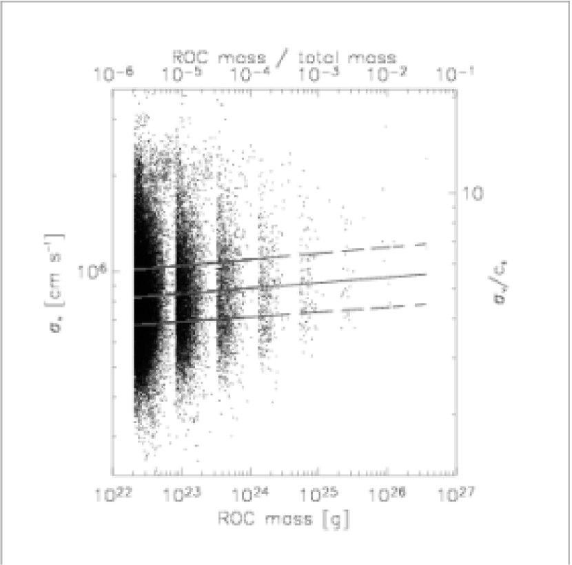
Figure 15: Sigma vs. mass of ROC, for $J=4\rightarrow 3$ molecular turbulence map. For reference, $c_{s}$ is the mass-weighted average speed of sound.

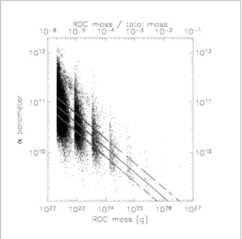
Figure 16: Alpha parameter vs. mass of ROC for $J=4\rightarrow 3$ molecular turbulence map

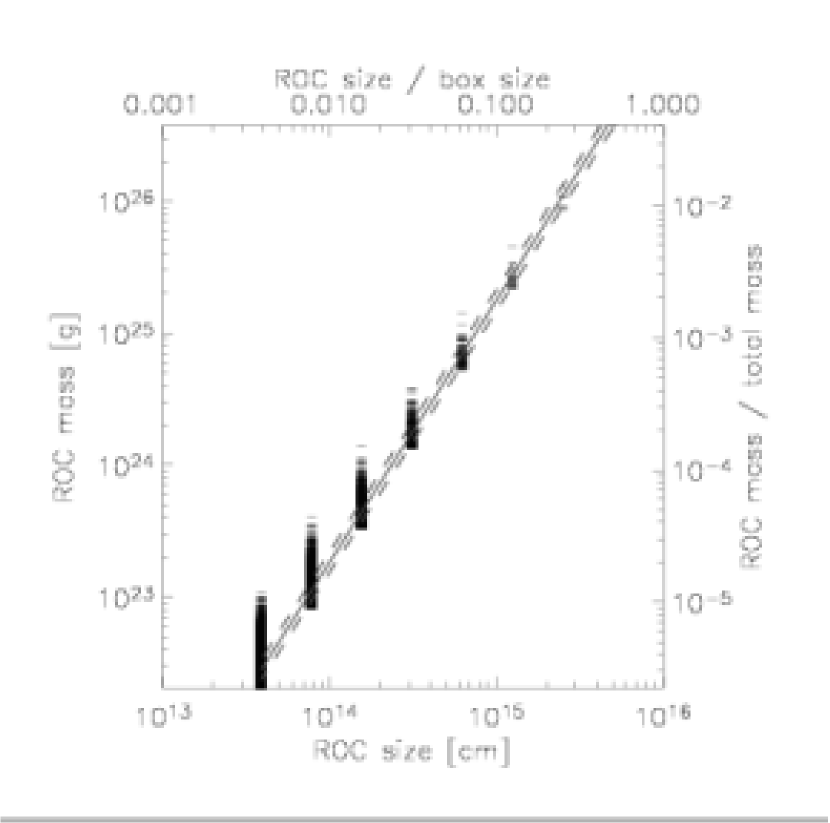
Figure 17: Mass of ROC vs. size of ROC, for $J=4\rightarrow 3$ molecular turbulence map

As noted in § 5.2, the statistical properties of the emission map constructed using density and velocity distributions from the actual IT simulations are virtually the same. The value of parameters in that case are

$$\begin{split}b&=(1.7\pm 0.4)\times 10^{-2},\quad b^{\prime}=(1.1\pm 0.2)\times 10^{-2},\\ c&=-(4.99\pm 0.04)\times 10^{-1},\quad d=1.985\pm 0.002.\end{split}$$ (47)

Such a good agreement in the morphology and statistical properties of the maps is due to the very homogeneous distribution of molecules in the gas. At this stage of molecular turbulence evolution, $t=60$ yr, there are numerous dissociative shocks, and the mean characteristics would suggest that molecular turbulence should be very different from isothermal turbulence in many respects (at $t=60$ yr the average molecular hydrogen fraction is $\langle f\rangle=0.1$, and average temperature is $\langle T\rangle=630$ K). Despite this, the analysis of actual molecular emission maps provides evidence to the contrary.

Furthermore, the shapes of spectral lines in both cases are very similar. The line shapes are very roughly Gaussian, with exponential tails in many cases. Exponential tails have indeed been observed and can be theoretically explained by the intermittency of the velocity distribution (Falgarone et al., 1994).

The linewidth-size relationship found for the ROCs is very flat and does not correspond to that of Larson’s law described in § 5.1. This has been fully discussed by Ostriker et al. (2001), who determined that the least squares fit is associated with the superposition of density structure along the line of sight. The relation for actual clumps or cores is related to the lower envelope of the linewidth-size scatter plot, which has a slope of $\sim 0.3\pm 0.1$, toward the shallow end of the observed values given by equation 34.

A similar analysis of synthetic $\mathrm{CO_{J}}$(20–19) maps emphasises the differences between the isothermal and non-isothermal regimes. Emission maps in this $\mathrm{CO}$ line are drastically different, as displayed in Fig. 18. The peak intensity in the isothermal case is a factor of more than $10^{3}$ lower. This is to be expected, as the $J=20\rightarrow 19$ transition traces only those regions where the gas has $T\approx 1000$ K. In the case of MT, hot regions are naturally associated with strong shocks, whereas in the (quasi-) isothermal case the temperature is much lower and uniform. Therefore, in the isothermal case, the emission in this line simply reflects the column density (compare the lower maps of Figs. 13 and 18).

For the $J=20\rightarrow 19$ emission maps, the values of parameters (41) — (44) are again given by least-square fits. Emission maps based on the MT simulation data yield

$$\begin{split}b&=(4.7\pm 0.4)\times 10^{-2},\quad b^{\prime}=(2.7\pm 0.2)\times 10^{-2},\\ c&=-(5.01\pm 0.04)\times 10^{-1},\quad d=1.950\pm 0.002.\end{split}$$ (48)

and for the quasi-isothermal case,

$$\begin{split}b&=(6.2\pm 0.7)\times 10^{-2},\quad b^{\prime}=(2.7\pm 0.3)\times 10^{-2},\\ c&=-(5.71\pm 0.06)\times 10^{-1},\quad d=1.936\pm 0.007.\end{split}$$ (49)

. It is remarkable that statistical properties of the maps of $\mathrm{CO}$(20–19) as summarised by equations (48) and (49) do not reveal any differences between MT and IT, although the underlying maps are completely different. They are very similar to the parameters of $\mathrm{CO}$(4–3) emission, see Eqs. (45) – (47). Linewidth-size relationship is somewhat steeper for the $\mathrm{CO}$(20–19) maps, which might be related to the size of the statistical sample (number of ROCs is smaller for $J=20\rightarrow 19$ transition).

The $J=20\rightarrow 19$ emission line profiles derived from molecular data are somewhat different from the line profiles derived from the quasi-isothermal data, with the emission lines often more prominently peaked (though far weaker) in the quasi-isothermal case.

The remaining parameters are qualitatively similar to the parameters derived for the $J=4\rightarrow 3$ line emission maps. The virial parameter $\alpha$ is large ($\alpha>10^{10}$), confirming that the kinetic energy is the dominant form of energy in this turbulence regime, and the ‘cores’ on the maps (ROCs) are false cores which cannot be gravitationally confined. The fact that $c<0$ indicates that gravity is relatively more important for regions with small mass (i.e. of smaller size).

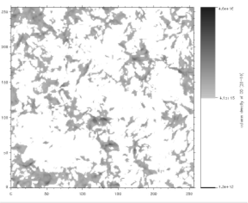
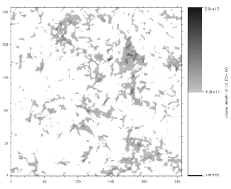
Figure 18: Maps of $\mathrm{{}^{12}CO}$ $J=20\rightarrow 19$ emission constructed from the MT data (upper panel). The same emission map constructed from the quasi-isothermal turbulence data (lower panel) as described in § 5.2. Note the huge difference in intensity as given by the colour bars.

The scale dependence of ROC mass and the virial parameter $\alpha$ have the following interpretation. In the limit of constant column density, the mass of a ROC of size $\lambda$ is $M\propto\rho_{\text{col}}\lambda^{2}$, where $\rho_{\text{col}}$ is the column density, and the resulting scale dependence is $M\propto\lambda^{2}$. These are close to the values we deduce from all emission maps, $M\propto\lambda^{d}$, where $d=1.96\pm 0.03$, as concluded also by Ballesteros-Paredes and Mac Low (2002). Scaling of the virial parameter $\alpha$ follows from the result for the mass scaling. Given that $\sigma$ is independent of $\lambda$, the scaling dependence of the parameter $\alpha$ approaches $\propto M^{-0.5}$ (in the limit of constant column densities). The numerical value is close to this limit: we find $\alpha\propto M^{c}$, where $c=-0.5\pm 0.2$.

5.4 Discussion

For molecular line emission that traces the bulk of the gas, isothermal simulations can be very accurate in mapping molecular emission. Properties of the emission maps and shapes of emission lines reproduce the corresponding values deduced from the detailed molecular simulations. An attempt to map shocked regions with a temperature-sensitive chemical tracer fails in the case of isothermal turbulence, as is naturally anticipated. Results of isothermal turbulence simulations should only be used for what they have been made — tracing gas close to the average temperature.

The predictions of values of scaling exponents from analysis of emission maps with different CO rotational number $J$ are approximately equal.

The algorithm for construction of synthetic emission maps used here is very simple. It functions only for the case of optically thin emission and may serve as a starting point for a deeper analysis. Self-consistent three-dimensional radiative transfer algorithms are essential for obtaining reliable predictions as, for example, used by Padoan et al. (1998) based on the radiative transfer code of Juvela (1997). The large velocity gradient approximation (Sobolev, 1957) for radiative transfer was used by Ossenkopf and Mac Low (2002) to construct synthetic emission maps.

6 CONCLUSIONS

We have examined how molecular dynamics influences supersonic turbulence and, vice versa, how turbulence influences molecular content. Numerical simulations of cloud dynamics have usually employed an isothermal equation of state as an approximation for gas inside molecular clouds. Hence, we have compared our results (MT) to that of the equivalent isothermal simulation (IT). We analysed decaying turbulence, beginning from a molecular state in which strong shocks develop and destroy 87% of the molecules and running until 80% of the molecules have reformed. Our main results are as follows.

1. There is no significant difference between the evolution of power spectra for MT and IT. The spectra are not power laws but involve a faster decay in the energy associated with the higher wavenumber regime.

2. Despite strongly supersonic root-mean-square velocities, the ratio of energy in compressional modes to energy in solenoidal modes at low wavenumbers drops from the initial value of 1:2 to $\sim$1:5 almost immediately. Little further decrease occurs at the low wavenumber end while the flow remains supersonic.

3. Compression waves steepen much faster in the simulation of molecular turbulence leading to a rapid increase in high wavenumber compressional energy. This appears to be due to the slower dissipation of thermal energy during the dissociative phase than in the equivalent isothermal phase. In contrast, the high wavenumber compressional energy in IT later overtakes that of the MT.

4. The effective polytropic index in MT varies considerably. In the very early stages, there are effectively two isothermal phases, corresponding to atomic gas at $\sim$ 8000 K and molecular gas at $\sim$ 40 K. The index is then reduced to below and above unity for extended periods (see Fig. 4) before approaching unity at late times. The sub-isothermal period is related to the presence of strong compression and molecule reformation behind fast shocks.

5. The density PDFs in the MT case are found to be close to log-normal. The strongest deviations occur early on when strong shocks distort the statistics. The deviations are smaller in the MT case than in IT, probably due to the higher effective polytropic index.

6. The structure of the velocity fields was studied with the help of the divergence and modulus of curl. Vortex isosurfaces take the form of sheets closely related in space and size to the shock surfaces.

7. The PDFs of vorticity, as well as velocity gradients, take the form of exponentials. We constructed PDFs of compensated distributions where the change of the mean values of the distributions is accounted for in the exponentials. With constant parameters, the functions provide a useful tool for diagnosing decaying turbulence. Velocity PDFs maintain Gaussian distributions.

8. Simulated maps of CO rotational emission lines are constructed. We find that isothermal simulations provide excellent agreement with the molecular predictions for tracers of the cool bulk of the gas. This is confirmed through the ‘Region of Contrast’ method to characterise the properties of the emission maps. In Paper I, we showed that as turbulence decays, molecules do not remain within swept-up shells but are distributed very homogeneously, and the molecular fraction distribution has a small variation. This results in very similar looking mass and molecular mass distributions during the reformation phase. On the basis of this result it is argued that isothermal simulations can be used to map molecules. This hypothesis is supported by the synthetic maps.

9. On the other hand, large differences are found in the emission distribution of high-J CO lines. These lines are sensitive to the temperature.

10. In astrophysical turbulence, the magnetic field influences turbulent cascades (Vestuto et al., 2003). For example, the column density power spectrum was found to be significantly shallower as the field strength is raised (Padoan et al., 2004). A strong magnetic field also enhances the shock number transverse to the field direction at the expense of parallel shocks (Smith et al., 2000a).

    The magnetic field would also weaken shocks, allowing molecules to survive the passage of stronger shocks. This will tend to reduce the differences with respect to the IT case caused by the chemical and cooling processes.

The main conclusion of this work is that isothermal simulations adequately model molecular turbulence and can be used to predict many properties of the molecular emission; given the supersonic dynamics, the chemical reactions in a turbulent gas can be significantly accelerated due to strong compression and advection.

This work provides a basis for future research in a number of directions. It is possible that the behaviour of molecules can be modelled as a passive scalar, and pseudo-temperature distributions can be constructed from appropriately gauged divergence fields.

7 Acknowledgements

We thank the anonymous referee for a careful report, and in particular for pointing out the work on PDF asymptotics. The computations reported here were performed using the UK Astrophysical Fluids Facility (UKAFF) and FORGE (Armagh), funded by the PPARC JREI scheme, in collaboration with SGI. M-MML was partially funded by the NASA Astrophysical Theory Program under grant number NAG5-10103 and NSF grants AST99-85392, and AST03-07793. GB has been partially funded by the PPARC. Armagh Observatory receives funding from the Northern Ireland Department of Culture, Arts and Leisure. ZEUS-3D was used by courtesy of the Laboratory of Computational Astrophysics at UC San Diego. This research has made use of NASA’s Astrophysics Data System Bibliographic Services.

References

- Ballesteros-Paredes and Mac Low (2002) J. Ballesteros-Paredes and M.-M. Mac Low. Physical versus Observational Properties of Clouds in Turbulent Molecular Cloud Models. ApJ, 570:734–748, May 2002.
- Balsara et al. (2004) D. S. Balsara, J. Kim, M.-M. Mac Low, and G. J. Mathews. Amplification of Interstellar Magnetic Fields by Supernova-driven Turbulence. ApJ, 617:339–349, Dec. 2004.
- Boldyrev (2002) S. Boldyrev. Kolmogorov-Burgers Model for Star-forming Turbulence. ApJ, 569:841–845, Apr. 2002.
- Boldyrev et al. (2002) S. Boldyrev, Å. Nordlund, and P. Padoan. Supersonic Turbulence and Structure of Interstellar Molecular Clouds. Phys. Rev. Lett., 89:31102, July 2002.
- Bonnell et al. (2003) I. A. Bonnell, M. R. Bate, and S. G. Vine. The hierarchical formation of a stellar cluster. MNRAS, 343:413–418, Aug. 2003.
- Bonnell et al. (2004) I. A. Bonnell, S. G. Vine, and M. R. Bate. Massive star formation: nurture, not nature. MNRAS, 349:735–741, Apr. 2004.
- Brunt et al. (2003) C. M. Brunt, M. H. Heyer, E. Vázquez-Semadeni, and B. Pichardo. Intrinsic, Observed, and Retrieved Properties of Interstellar Turbulence. ApJ, 595:824–841, Oct. 2003.
- Dgani et al. (1996) R. Dgani, D. van Buren, and A. Noriega-Crespo. The Transverse Acceleration Instability for Bow Shocks in the Nonlinear Regime. ApJ, 461:372, Apr. 1996.
- Elmegreen and Scalo (2004) B. G. Elmegreen and J. Scalo. Interstellar Turbulence I: Observations and Processes. ARA&A, 42:211–273, Sept. 2004.
- Falgarone et al. (1994) E. Falgarone, D. C. Lis, T. G. Phillips, A. Pouquet, D. H. Porter, and P. R. Woodward. Synthesized spectra of turbulent clouds. ApJ, 436:728–740, Dec. 1994.
- Frisch (1995) U. Frisch. Turbulence. Cambridge University Press, 1995.
- Frisch et al. (2001) U. Frisch, J. Bec, and B. Villone. Singularities and the distribution of density in the Burgers/adhesion model. Physica D Nonlinear Phenomena, 152:620–635, May 2001.
- Frisch and Beck (2001) U. Frisch and J. Beck. Burgulence. In M. Lesieur, A. Yaglom, and F. David, editors, New Trends in Turbulence: Les Houches 2000, pages 341–383. Springer EDP-Sciences, 2001.
- Gotoh and Kraichnan (1993) T. Gotoh and R. H. Kraichnan. Statistics of decaying Burgers turbulence. Physics of Fluids, 5:445–457, Feb. 1993.
- Gotoh and Kraichnan (1998) T. Gotoh and R. H. Kraichnan. Steady-state Burgers turbulence with large-scale forcing. Physics of Fluids, 10:2859–2866, Nov. 1998.
- Heyer and Schloerb (1997) M. H. Heyer and F. P. Schloerb. Application of Principal Component Analysis to Large-Scale Spectral Line Imaging Studies of the Interstellar Medium. ApJ, 475:173, Jan. 1997.
- Juvela (1997) M. Juvela. Non-LTE radiative transfer in clumpy molecular clouds. A&A, 322:943–961, June 1997.
- Klessen (2000) R. S. Klessen. One-point probability distribution functions of supersonic turbulent flows in self-gravitating media. ApJ, 535:869–886, June 2000.
- Larson (1981) R. B. Larson. Turbulence and star formation in molecular clouds. MNRAS, 194:809–826, Mar. 1981.
- Lazarian et al. (2001) A. Lazarian, D. Pogosyan, E. Vázquez-Semadeni, and B. Pichardo. Emissivity Statistics in Turbulent Compressible Magnetohydrodynamic Flows and the Density-Velocity Correlation. ApJ, 555:130–138, July 2001.
- Lesieur (1997) M. Lesieur. Turbulence in Fluids. Kluwer Academic Publishers, third revised and enlarged edition (2000) edition, 1997.
- Lesieur et al. (2003) M. Lesieur, P. Begou, E. Briand, A. Danet, F. Delcayre, and J. L. Aider. Coherent-vortex dynamics in large-eddy simulations of turbulence. Journal of Turbulence, 4:16, Apr. 2003.
- Li et al. (2003) Y. Li, R. S. Klessen, and M.-M. Mac Low. The Formation of Stellar Clusters in Turbulent Molecular Clouds: Effects of the Equation of State. ApJ, 592:975–985, Aug. 2003.
- Mac Low and Klessen (2004) M.-M. Mac Low and R. S. Klessen. Control of star formation by supersonic turbulence. Reviews of Modern Physics, 76:125–194, Jan. 2004.
- Mac Low et al. (1998) M.-M. Mac Low, R. S. Klessen, A. Burkert, and M. D. Smith. Kinetic Energy Decay Rates of Supersonic and Super-Alfvénic Turbulence in Star-Forming Clouds. Phys. Rev. Lett., 80:2754–2757, Mar. 1998.
- Mac Low and Norman (1993) M.-M. Mac Low and M. L. Norman. Nonlinear growth of dynamical overstabilities in blast waves. ApJ, 407:207–218, Apr. 1993.
- Mac Low and Ossenkopf (2000) M.-M. Mac Low and V. Ossenkopf. Characterizing the structure of interstellar turbulence. A&A, 353:339–348, Jan. 2000.
- Mac Low et al. (2005) M.-M. Mac Low, D. S.Balsara, J. Kim, and M. A. de Avillez. The title. ApJ, in press, Mar. 2005.
- McKee et al. (1982) C. F. McKee, J. W. V. Storey, D. M. Watson, and S. Green. Far-infrared rotational emission by carbon monoxide. ApJ, 259:647–656, Aug. 1982.
- McKee and Zweibel (1992) C. F. McKee and E. G. Zweibel. On the virial theorem for turbulent molecular clouds. ApJ, 399:551–562, Nov. 1992.
- Ossenkopf and Mac Low (2002) V. Ossenkopf and M.-M. Mac Low. Turbulent velocity structure in molecular clouds. A&A, 390:307–326, July 2002.
- Ostriker et al. (2001) E. C. Ostriker, J. M. Stone, and C. F. Gammie. Density, velocity, and magnetic field structure in turbulent molecular cloud models. ApJ, 546:980–1005, Jan. 2001.
- Padoan et al. (2003) P. Padoan, S. Boldyrev, W. Langer, and Å. Nordlund. Structure Function Scaling in the Taurus and Perseus Molecular Cloud Complexes. ApJ, 583:308–313, Jan. 2003.
- Padoan et al. (2004) P. Padoan, R. Jimenez, M. Juvela, and Å. Nordlund. The Average Magnetic Field Strength in Molecular Clouds: New Evidence of Super-Alfvénic Turbulence. ApJ, 604:L49–L52, Mar. 2004.
- Padoan et al. (1997) P. Padoan, B. J. T. Jones, and A. P. Nordlund. Supersonic Turbulence in the Interstellar Medium: Stellar Extinction Determinations as Probes of the Structure and Dynamics of Dark Clouds. ApJ, 474:730, Jan. 1997.
- Padoan et al. (1998) P. Padoan, M. Juvela, J. Bally, and A. Nordlund. Synthetic Molecular Clouds from Supersonic Magnetohydrodynamic and Non-LTE Radiative Transfer Calculations. ApJ, 504:300, Sept. 1998.
- Padoan and Nordlund (2002) P. Padoan and Å. Nordlund. The Stellar Initial Mass Function from Turbulent Fragmentation. Apj, 576:870–879, Sept. 2002.
- Passot and Vázquez-Semadeni (1998) T. Passot and E. Vázquez-Semadeni. Density probability distribution in one-dimensional polytropic gas dynamics. Phys. Rev. E, 58:4501–4510, Oct. 1998.
- Pavlovski et al. (2002) G. Pavlovski, M. D. Smith, M.-M. Mac Low, and A. Rosen. Hydrodynamical simulations of the decay of high-speed molecular turbulence. I. Dense molecular regions. MNRAS, 337:477–487, 2002.
- Pichardo et al. (2000) B. Pichardo, E. Vázquez-Semadeni, A. Gazol, T. Passot, and J. Ballesteros-Paredes. On the Effects of Projection on Morphology. ApJ, 532:353–360, Mar. 2000.
- Porter et al. (2002) D. Porter, A. Pouquet, and P. Woodward. Measures of intermittency in driven supersonic flows. Phys.Rev. E, 66(2):026301, Aug. 2002.
- Scalo et al. (1998) J. Scalo, E. Vázquez-Semadeni, D. Chappell, and T. Passot. On the Probability Density Function of Galactic Gas. I. Numerical Simulations and the Significance of the Polytropic Index. ApJ, 504:835, Sept. 1998.
- Smith et al. (2000a) M. D. Smith, M.-M. Mac Low, and F. Heitsch. The distribution of shock waves in driven supersonic turbulence. A&A, 362:333–341, Oct. 2000a.
- Smith et al. (2000b) M. D. Smith, M.-M. Mac Low, and J. M. Zuev. The shock waves in decaying supersonic turbulence. A&A, 356:287–300, 2000b.
- Smith et al. (2004) M. D. Smith, G. Pavlovski, M.-M. Mac Low, T. Khanzadyan, R. Gredel, and T. Stanke. Molecule destruction and formation in molecular clouds. Ap. & Sp. Sci., pages 333–336, Jan. 2004.
- Smith and Rosen (2003) M. D. Smith and A. Rosen. The instability of fast shocks in molecular clouds. MNRAS, 339:133–147, Feb. 2003.
- Sobolev (1957) V. V. Sobolev. The Diffusion of L Radiation in Nebulae and Stellar Envelopes. Soviet Astronomy, 1:678, Oct. 1957.
- Stone and Norman (1992) J. M. Stone and M. L. Norman. ZEUS-2D: A radiation magnetohydrodynamics code for astrophysical flows in two space dimensions. I. The hydrodynamical algorithms and tests. ApJS, 80:753–790, 1992.
- Tilley and Pudritz (2004) D. A. Tilley and R. E. Pudritz. The formation of star clusters - I. Three-dimensional simulations of hydrodynamic turbulence. MNRAS, 353:769–788, Sept. 2004.
- Titon and Cadot (2003) J. H. Titon and O. Cadot. Direct measurements of the energy of intense vorticity filaments in turbulence. Phys. Rev. E, 67:27301, Feb. 2003.
- Vázquez-Semadeni (1994) E. Vázquez-Semadeni. Hierarchical Structure in Nearly Pressureless Flows as a Consequence of Self-similar Statistics. ApJ, 423:681, Mar. 1994.
- Vázquez-Semadeni et al. (1997) E. Vázquez-Semadeni, J. Ballesteros-Paredes, and L. F. Rodriguez. A Search for Larson-Type Relations in Numerical Simulations of the ISM: Evidence for Nonconstant Column Densities. ApJ, 474:292, Jan. 1997.
- Vázquez-Semadeni et al. (1996) E. Vázquez-Semadeni, T. Passot, and A. Pouquet. Influence of Cooling-induced Compressibility on the Structure of Turbulent Flows and Gravitational Collapse. ApJ, 473:881, Dec. 1996.
- Vestuto et al. (2003) J. G. Vestuto, E. C. Ostriker, and J. M. Stone. Spectral Properties of Compressible Magnetohydrodynamic Turbulence from Numerical Simulations. ApJ, 590:858–873, June 2003.
- Vishniac (1983) E. T. Vishniac. The dynamic and gravitational instabilities of spherical shocks. ApJ, 274:152–167, Nov. 1983.
- Vishniac (1994) E. T. Vishniac. Nonlinear instabilities in shock-bounded slabs. ApJ, 428:186–208, June 1994.