Pushing the Limits of Ground-Based Photometric Precision – Sub-Millimagnitude Time-Series Photometry of the Open Cluster NGC 6791

Abstract

We present the results from a three night, time-series study of the open cluster NGC 6791 using the Megacam wide-field mosaic CCD camera on the 6.5m MMT telescope. The aim of this study was to demonstrate the ability to obtain very high precision photometry for a large number of stars. We achieved better than 1% precision for more than 8000 stars with $14.3<R<20.1$ and sub-millimagnitude (as low as 360 $\mu$mag) precision for over 300 stars with $14.6<R<16.3$ in the field of this cluster. We also discovered 8 new variable stars, including a possible $\delta$-Scuti variable with an amplitude of 2%, 6 likely W UMa contact binaries, and a possible RS CVn star, and we identified 5 suspected low-amplitude variables, including one star with an amplitude of 3 mmag. We comment on the implications of this study for a ground-based survey for transiting planets as small as Neptune.

1 Introduction

Since the advent of high quality CCDs there has been a great deal of effort to obtain high-precision (millimagnitude, or less than 1%) time-series, optical and infrared photometry for large numbers of stars. Photometry at the millimagnitude level of precision is considered a prerequisite in searches for transiting Jupiter-sized planets around solar-type stars. As a result, the number of groups that have achieved this level of precision is too many to list here (see for example Horne 2003 for a list of transiting planet searches). The search for transiting planets has not been in vain; at the time of writing there are 7 known transiting planets, 6 of which were first identified photometrically (see e.g. Udalski et al. 2004 and Konacki et al. 2004). Millimagnitude photometry has also contributed to the study of stars near the hydrogen fusion limit (Pont et al., 2005) and enabled the study of stellar variability with amplitudes of a few percent (e.g. Bruntt et al. 2003). With the number of transit surveys growing steadily, millimagnitude photometry has become routine. Pushing below $0.1$%, however, has proven difficult.

To our knowledge, Gilliland et al. (1993) holds the record for the most precise (per exposure) ground-based photometry that has been reported. They achieved a precision as good as 250 $\mu$mag per exposure for a group of 12 stars in M67 that they monitored for solar-like oscillations. Prior to that, Gilliland & Brown (1992) achieved a precision of 750 $\mu$mag per exposure. In both of these cases only a handful of bright isolated stars were monitored. Since these projects were aimed at searching for short time-scale, solar-like oscillations, the authors applied high-pass filters to their light curves, thereby removing any long time-scale systematic trends together with any long time-scale variability. Ground-based, sub-millimagnitude per exposure photometry has also been obtained for individual bright objects (e.g. Jha et al. 2000 who obtained an RMS of 800 $\mu$mag for the transiting system HD209458 using a photometer; also see Kurtz et al. 2005).

Despite the difficulties in performing sub-millimagnitude photometry from the ground for large numbers of stars, the possible science rewards are compelling. Improving the precision of transit surveys by a factor of ten would allow for the detection of $0.1$% transits due to Neptune-sized planets orbiting solar-type stars. It would also allow the exploration of a new regime of stellar variability.

As discussed in the next section, the Megacam instrument on the MMT telescope is an ideal setup for achieving sub-millimagnitude photometry from the ground. Motivated by the possibility of opening a new regime to ground-based, time-series campaigns, we set out to demonstrate photometry for a large number of stars with a per-exposure precision as good as a few parts in 10,000 by conducting a short time-series study of the open cluster NGC 6791 using MMT/Megacam.

In the following section we describe our observations. We follow with a discussion of our data reduction steps in §3; in §4 we describe the photometric precision we have achieved; in §5 we present new variable stars that we have found in this field; and we finish with a discussion of our results, including the possibility of a search for transiting Neptune-sized planets in §6.

2 Observations

The data for this project were obtained on the nights of October 4th, 9th and 20th of 2004 using the Megacam CCD mosaic (McLeod et al., 2000) mounted on the MMT 6.5m telescope. The Megacam instrument is a $24\arcmin$ x $24\arcmin$ mosaic consisting of 36 2k$\times$4k, thinned, backside-illuminated CCDs that are each read out by two amplifiers. The mosaic has a pixel scale of $0.08\arcsec$ which allows for a well sampled point-spread-function (PSF) even under the best seeing conditions. The result is that in $1\arcsec$ seeing one can collect as many as $2\times 10^{7}$ photons from a single star prior to saturation, setting the photon limit for the precision in a single exposure at 0.25 mmag.

For this study we chose to observe the open cluster NGC 6791. This cluster has been studied extensively for variability by the PISCES project (Mochejska et al. 2002, 2005, additional variability surveys of this cluster include those by Kaluzny & Ruciński 1993, Ruciński, Kaluzny, & Hilditch 1996, Mochejska, Stanek, & Kaluzny 2003, and Bruntt et al. 2003). As noted in Mochejska et al. 2005, the cluster is populous (Kaluzny & Udalski, 1992), old ($\tau=8$Gyr), metal rich ([Fe/H]=$+0.4$), and located at a distance modulus of (m-M)${}_{V}=13.42$ (Chaboyer, Green, & Liebert, 1999).

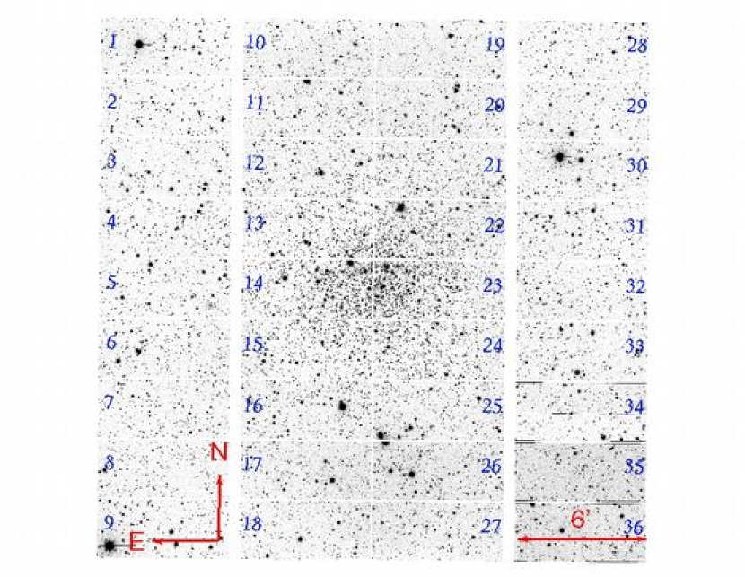
Figure 1: Megacam mosaic image of the open cluster NGC 6791. Chip labels are for reference in the text.

We obtained 71 exposures centered on the cluster $(\alpha,\delta)=(19^{\rm h}20^{\rm m}53\fs 0,+37\arcdeg 46\arcmin 30\farcs 0)$ (J2000.0) using a Sloan-$r^{\prime}$ filter. Of these exposures, 20 were obtained on Oct. 04, 2004 with a two minute exposure time, 17 on Oct. 09, 2004 with a two minute exposure time, and 36 on Oct. 20, 2004 with a one minute exposure time. The data on the first two nights were obtained with a gain setting of 10 e^-/ADU, after noting the possibility of nonlinearity in pixels with more than $2\times 10^{5}$ e^- we switched to a gain of 3.5 e^-/ADU for the last night. In both cases we were not limited by the A/D converter. All images were read-out using 2x2 binning (yielding a pixel scale $0.16\arcsec$), but this did not limit the number of electrons in the detector. For reference, we present a Megacam mosaic image of the field in Fig. 1.

For the first night the seeing was highly variable, ranging from $1\arcsec$ to $3\arcsec$. On the second and third nights the seeing was relatively stable, but not exceptional, and ranged from $1\arcsec$ to as high as $2\arcsec$ in a handful of images. The poor conditions on the first night make the data unusable for precision photometry using our reduction techniques, though we include data from this night in the light curves presented in §5.

3 Data Reduction

The preliminary CCD reductions, including overscan, zero level correction, and flat-fielding were performed using the standard routines in the IRAF MSCRED package. For each night we constructed a master twilight flat-field from 5, 19, and 5 individual twilight flat-field exposures, respectively.

To obtain photometry we used the image subtraction methods due to Alard & Lupton (1998; see also Alard 2000) as implemented in the ISIS 2.1 package. The procedure we followed is similar to that described in e.g. Hartman et al. (2004); here we only highlight differences from the procedure discussed there. The basic scheme is to match the PSF and background of a reference image to another image, subtract them, and perform photometry on the subtracted image. The photometry routine that comes with the ISIS package convolves a PSF determined empirically on the reference image with the convolution kernel used to match the images, and then performs fixed-position, PSF fitting photometry on the subtracted image.

We performed subtraction independently for 33 of the 36 CCDs in the mosaic (the three chips labelled 34-36 in Fig. 1 had artifacts that rendered them unusable at the time), dividing each CCD into two independent sub-regions. We created saturation masks for each image, so that pixels above 60,000 ADU would not be used in the photometry extraction routines. Prior to registering the images we binned them 3x3. This reduced the full width at half maximum (FWHM) of the PSF to 2-3 pixels over the range of seeings that were encountered, and thus allowed us to use the existing ISIS routines without substantial modification. Reference images for each chip were created from the best seeing images on the third night.

Because one only measures differential flux with image subtraction, it is necessary to obtain base fluxes for the stars via another technique if one wishes to obtain light curves in magnitudes. We obtained these fluxes by performing PSF photometry on the reference images for each chip using DAOPHOT/ALLSTAR (Stetson 1987, 1992). To ensure that the fluxes that we measured in ISIS are on the same scale as those measured with DAOPHOT/ALLSTAR, we performed an aperture correction by measuring the flux on the reference images using aperture photometry with a radius equal to that used in ISIS, and adjusting the PSF photometry to remove any systematic differences from the aperture photometry. The corrections were typically less than 0.1mag (in absolute value), and all had an RMS uncertainty less than 10 mmag. As a result, any systematic error in the amplitudes should be less than $1$% of the stated amplitude.

We proceeded to obtain photometry for 27,885 stars on 33 CCDs with $13.9<R<24.0$. We calibrated the photometry to the R-band using data provided to us from PISCES (B. Mochejska, private communication, 2005). Having obtained the light curves, we performed two cleaning steps. The first step was to remove any systematic changes in the zero-points of the light curves. We did this by solving for the corrections to the zero-points that minimize

$$\sum_{i,j}\frac{(m_{ij}+\Delta z_{i}-\bar{m_{j}})^{2}}{\sigma_{ij}^{2}},$$ (1)

where $m_{ij}$ is the magnitude of the $j$th star at time $i$, $\bar{m_{j}}$ is the average magnitude of the $j$th star, $\sigma_{ij}$ is the uncertainty in the magnitude of the $j$th star at time $i$ and is calculated assuming photon noise and the gain listed in the Megacam Observers Manual, and $\Delta z_{i}$ is the correction to the zero-point at time $i$. The zero-point corrections were all less than 1 mmag and hence only affected the precision of the brightest stars. In the second step we rejected observations, for each chip, for which a substantial percentage of stars on the chip (more than 4.5%) showed a greater than $3\sigma$ deviation from their mean. This removed 3 or 4 of the 36 observations on the third night for most of the chips. The rejected observations were among the poorest seeing images for the night. For the second night we used a less stringent criterion of 19% to remove 1 or 2 of the 17 observations for most of the chips. We required a less stringent criterion because a greater fraction of the stars for which we extracted photometry were saturated in the longer exposures of the second night.

Even with the aperture correction it is still possible for there to be a systematic error in the amplitudes of variations. This would happen, for example, if there was a systematic error in the ISIS photometry that might result from errors in the subtraction process. To ensure that we are not underestimating the amplitudes of our light curves, and hence overestimating our precision, we extracted photometry for a handful of simulated variable stars.

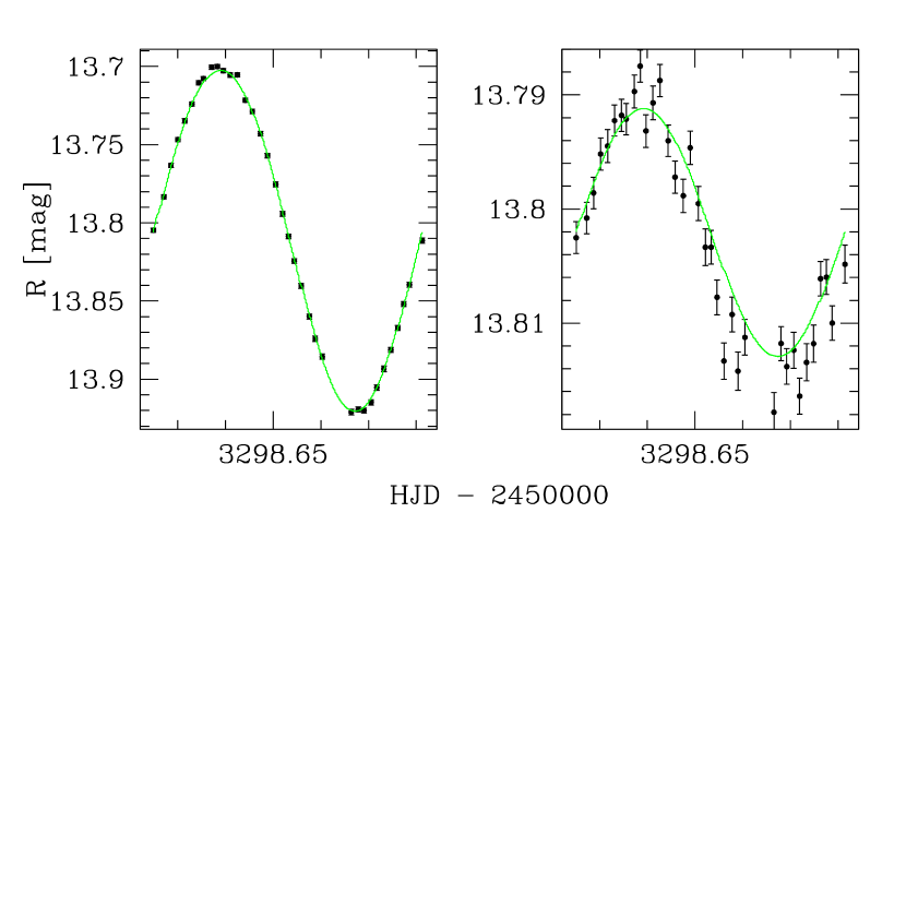
Figure 2: Light curves of simulated variable stars. Points were extracted using image subtraction, the solid line shows the input variable star signal. The noise in the light curve comes from the base star that is multiplied by the signal, as well as from errors in the simulation process. At left is a 10% semi-amplitude variation, at right is a 1% semi-amplitude variation. Note that the amplitude of the measured light curve is not less than that of the input signal.

To add the simulated variable stars we first identified a bright isolated star on one of the images and extracted a small box around the star in every image. We then measured and subtracted the sky from the box, multiplied the box by a scaling factor and added the result to another location on the image. In this way we simulated two variables stars with semi-amplitude flux-variations of 10%, and 1%. We present the resulting light curves in Fig. 2. The purpose of this procedure was to test for systematic errors in the amplitudes, we stress that the overall noise in the light curves is not representative of noise expected for stars of this brightness as extra noise is introduced in the sky subtraction process. As is apparent from Fig. 2, the light curves are in good agreement with the simulated signal.

4 Photometric Precision

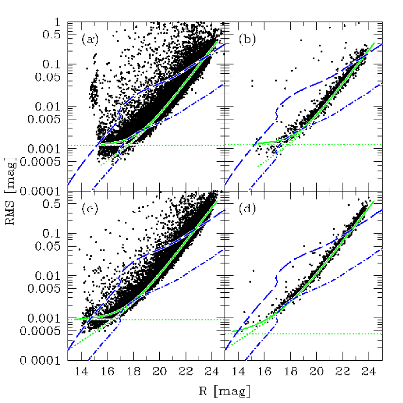
Figure 3: The light curve RMS versus magnitude is plotted for (a) chips 1-33 on night 2, (b) chip 21 on night 2, (c) chips 1-33 on night 3, and (d) chip 21 on night 3. The solid line shows a fit to the observed errors including photon noise and a constant error term (dotted lines), the dashed line shows the 6.5$\sigma$ detection limit for a transiting Jupiter-sized planet, while the dot-dashed line shows the same limit for a transiting Neptune-sized planet. The generation of these lines is described in §4 and we discuss the implications in §6.

In Fig. 3 we plot the RMS of each light curve versus the average magnitude for that light curve. We plot each night separately, for both the entire mosaic and the best individual chip (labeled 21 in Fig. 1).

For reference we also plot the $6.5\sigma$ detection limits for Jupiter and Neptune sized transiting planets. These lines are defined by eq. [3] in Mochejska et al. (2002)

$${\rm RMS}=\sqrt{N}\Delta R/\sigma,$$ (2)

where $N$ is the number of observations in transit, $\Delta R$ is the amplitude of the transit, and $\sigma$ is set to $6.5$. To calculate $N$ we use the length of a transit as given by eq. [1] of Gilliland et al. (2000)

$$\tau=1.412M_{*}^{-1/3}R_{*}P^{1/3},$$ (3)

where $\tau$ and $P$ are in days, and the stellar mass, $M_{*}$, and radius, $R_{*}$, are in solar units. To obtain $M_{*}$ and $R_{*}$ as functions of magnitude we generated isochrones from Girardi et al. (2000) using the parameters for the cluster listed in §2. The lines were then calculated for a $P=3.5$day period planet assuming one observes 3 full transits with two minute integrations taken every 3 minutes for comparison with night 2, and one minute integrations taken every 2 minutes for comparison with night 3. The implications of these lines are discussed in §6.

There are a total of 378 stars that have RMS $<$ 1 mmag on the second night, and 9661 with RMS $<$ 10 mmag. For the third night, with the shorter exposure times, we find 365 stars with RMS $<$ 1 mmag and 8132 with RMS $<$ 10 mmag. When the two nights are combined we find only 65 stars with RMS $<$ 1 mmag and 7732 with RMS $<$ 10 mmag. The drastic reduction in the number of stars with RMS $<$ 1 mmag is not unexpected as the differing exposure times between the two datasets results in a different saturation level.

From Fig. 3 it is clear that the observed RMS values are consistent with photon statistics for all but the brightest magnitudes. For stars brighter than $R=16$ mag there appears to be an additional source of error contributing to the RMS. To determine this constant error for each chip on the second and third nights we estimated the RMS in magnitudes of the jth light curve as:

$$\sigma_{j}=\sqrt{\sum_{i=1}^{n}\frac{(2.5\log_{10}({\rm e}))^{2}(F_{ji}+s_{i})}{g_{eff}\cdot n\cdot F_{ji}^{2}}+c^{2}},$$ (4)

where $n$ is the number of images, $F_{ji}=10^{2(z_{i}-m_{ji})/5}$ is the flux in ADU of the $j$th light curve on the $i$th image, $z_{i}$ is the zero-point of the $i$th image, $m_{ji}$ is the magnitude of the $j$th light curve on the $i$th image, $s_{i}$ is the effective sky flux of the $i$th image, $g_{eff}$ is the effective gain of the chip, and $c$ is the constant error term for the chip. When performing PSF fitting the above equation is applicable except that the effective gain is less than the actual gain, with the exact factor depending on the shape of the PSF and the size of the region one uses to fit the PSF (see Kjeldsen & Frandsen 1992 eq. [37] for the case of a Gaussian PSF). We find values for the effective gain that are typically less than the actual gain of the CCD by a factor of $\sim 1.7$.

We find that on the second night the constant error term ranges from 0.56 mmag to 2.4 mmag with an average value (over stars) of 1.2 mmag, while for the third night the constant error term ranges from 0.42 mmag to 1.6 mmag with an average value of just below 1 mmag. We also note that stars faint enough for the errors to be dominated by photon statistics have a lower RMS in the second night compared to the third by a factor that is consistent with the longer exposure time for the second night.

When the data for the second and third nights are combined, the RMS is not increased for stars that are below saturation in both nights ($R<15.5$). This implies that there is no substantial systematic offset between the nights and suggests that one may be able to consistently achieve this level of precision for a longer time series campaign.

There are a number of possible sources for the observed constant error term in our photometry. The relative error in the photometry (in magnitudes) due to Poisson noise in the flat-field is (Kjeldsen & Frandsen, 1992):

$$c_{ff}=\frac{2.5\log_{10}({\rm e})}{N_{ff}^{1/2}}$$ (5)

where $N_{ff}=\Omega_{eff}e_{ff}$, $\Omega_{eff}$ is the effective area of the PSF in pixels, and $e_{ff}$ is the total number of electrons in the flat-field in one pixel. For the third night the combined flat-field has $e_{ff}=3.3\times 10^{5}$ electrons/2x2 pixel, and the FWHM ranged from 6 to 12 2x2 pixels. Thus the expected constant error term due to flat-fielding lies below 0.2 mmag, well below the measured constant error terms for that night. This calculation assumes that the flat-fielding error is dominated by shot noise, the actual error may be larger if there are other systematic errors in the flat-field. The effect of this error is reduced when the pointing is stable between images. We note that because the PSF is so well-sampled on the Megacam CCDs we do not expect intra-pixel variations in the quantum efficiency to make a significant contribution to the error.

Atmospheric scintillation also adds an effective constant error term to the photometry. This error can be estimated from Young (1967) as

$$c_{scint}=0.1d^{-2/3}X^{1.75}\exp(-h/8000)(2t_{exp})^{-1/2}$$ (6)

where we use $c_{scint}$ for the constant error term due to scintillation, $d$ is the telescope diameter in cm, $X$ is the airmass, $h$ is the observatory altitude in m, and $t_{exp}$ is the exposure time in s. The leading coefficient is rather approximate (we multiply by $2.5\log_{10}({\rm e})$ to convert to magnitudes), as scintillation can change by a factor of 2 in a few minutes (e.g. Young 1993). For the second night, our observations were 60 seconds long, with the airmass ranging from 1.12 to 1.37. The MMT is located at an altitude of 2606 m, and has a diameter of 650 cm. Therefore we expect a constant error term of less than about 0.15 mmag due to atmospheric scintillation, and thus the total constant error term should be less than 0.25 mmag.

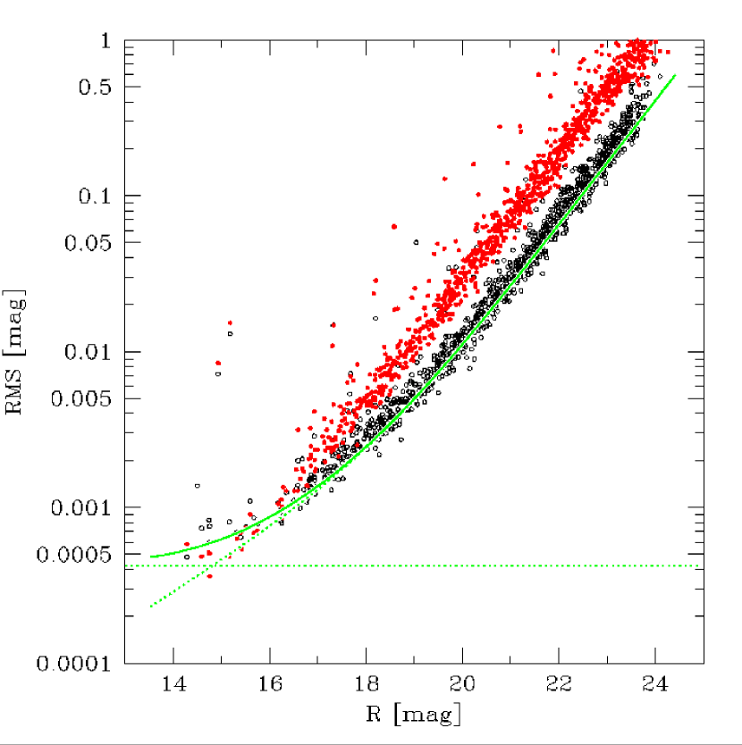
Figure 4: Comparison between the precision from performing aperture photometry on the subtracted images (filled points) and PSF photometry on the subtracted images (open circles) for chip 21. The curves are the same as those in Fig. 3 (c). Note that aperture photometry apears to provide better precision for the brightest stars, while it provides worse photometry for fainter stars as the result of an effectively higher sky flux through the unweighted aperture.

Because one obtains the PSF only once on the reference, the error in the PSF will not contribute to the errors in differential photometry. Instead, errors in the kernel that is used to convolve the PSF effectively add a constant error term to the photometry. It is difficult to estimate a priori exactly what that error should be, and we suspect that the constant error term that we have measured is due to this effect. To test this hypothesis we have also performed simple unit-weight aperture photometry on the subtracted images, the results for a single chip on the third night are shown in Fig 4. To correctly scale the fluxes we divided by the integral of the PSF over the aperture radius. We varied the aperture radius to optimize the precision at the bright end while providing correct amplitudes for the simulated variable stars mentioned in the previous section. The aperture photometry light curves were then put through the cleaning procedures described in the previous section to provide a fair comparison with the optimal PSF light curves. As expected, unit-weight aperture photometry performs worse than PSF fitting for faint stars as it is subject to a greater degree of sky background, however for the brightest stars aperture photometry outperforms PSF fitting, and appears to show no evidence of a constant error term. This effect is well-known when not using image subtraction, and confirms our suspicions that the constant error term arises from uncertainties in the kernel propagated through PSF fitting. Using aperture photometry on the subtracted images we achieve a precision as good as 360 $\mu$mag per exposure.

5 Variable Stars

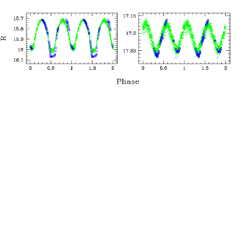
Figure 5: Comparison between our light curves (open circles) and those from PISCES (closed circles) for a few known variable stars: (left) V1 (right) V4. An arbitrary constant has been added to our light curves to provide alignment with the PISCES light curves.

As a check on our photometry we compare our light curves for a few known variables with those published by Mochejska et al. (2005) in Fig. 5. It is clear from the light curves that our photometry matches well.

While the short time coverage of our observations prevents us from performing a systematic survey for variable stars, we have identified 8 new variables in the field of NGC 6791 and 5 suspected variables that show evidence for low-amplitude variability. Table 1 lists the coordinates and basic photometric data for these variables, which we identify as V115-V122 and SV1-SV5. These stars were selected for their short period variability using the Schwarzenberg-Czerny algorithm (Schwarzenberg-Czerny, 1996) as implemented in a code due to Devor (2005).

We present phased light curves for the newly discovered variables in Fig. 6. For some of the suspected variable stars we have omitted the data from the first night when the noise is greater than the amplitude of variability in the second two nights. Due to a lack of time coverage the periods are tentative.

From the light curves we classify V116, V117, and V119-V122 as likely W UMa type contact binary systems. The variable V115 has a period and light curve shape that is typical of a $\delta$-Scuti type pulsating star. Lacking color information for this star, we cannot verify whether this identification is correct. We note that differences between the variations on the three days shows possible evidence for multiple modes of pulsation. Also note the precision of this 20 mmag amplitude light curve, particularly for the second and third nights. The light curve of V118 is similar to that of an RS CVn type spotted star. All of these variables lie outside of the field studied by PISCES which is why they were not detected by that project.

The suspected variables (SV1-SV5) show very small full-amplitude variations, as low as 3 mmag in the case of SV1. Of these, only SV2 lies within the field studied by PISCES. If real, the detection of these subtle variations represents an exciting demonstration of the potential of MMT/Megacam for precision time-series campaigns. At present, with a limited amount of data, we cannot rule out the possibility that some of these variations are the result of trends in the data rather than actual stellar variability as we have made no attempt to correct for color-dependent extinction or correlations with pixel-position.

6 Discussion

We have successfully demonstrated the capability of the MMT/Megacam to achieve very high precision photometry, as low as 360 $\mu$mag at the bright end, for a large number of stars. In the process we have discovered 8 new variable stars, and have identified 5 possible variable stars with amplitudes as low as 3 mmag. While we have not broken the record so to speak for the best precision per exposure obtained from the ground, we have achieved sub-millimagnitude photometry from the ground for more stars at once than has ever been reported. Our results with aperture photometry on the subtracted images shows that there are no barriers to our ability to achieve precisions of a few hundred micromagnitudes with this telescope and instrument.

While the detectection of solar-like, p-mode oscillations in other stars is difficult to do in a reasonable amount of time, even with sub-millimagnitude photometry (see for example Gilliland et al. 1993), we can still probe a relatively unexplored regime of stellar variability.

Another exciting application of this technology could be to survey stellar clusters for planets as small as Neptune. In Figures 3-4 we showed the 6.5$\sigma$ detection limits for planets as small as Neptune assuming one observed 3 full transits with MMT/Megacam. For the second night, with the two minute exposure time, there are 23,062 stars below the Jupiter detection limit, and 1664 stars below the Neptune detection limit. On the third night, with the 1 minute exposures, there are 19,843 stars below the Jupiter detection limit, and 648 stars below the Neptune detection limit. We have made no attempt here to distinguish between field stars and cluster members.

The ability to detect Jupiters in this system is not limited by precision but rather the time baseline over which observations are carried out. If one observes long enough to have a resonable chance of detecting 2-3 full transits, then one would be able to find essentially every short-period, transiting, Jupiter-sized planet in the stellar cluster. Since there are only three known planets with a lower mass-limit near that of Neptune (Santos et al., 2004; McArthur et al., 2004; Butler et al., 2004), essentially nothing is known about the statistics of Neptune-sized planets. Moreover, because all of these planets have been detected only via their influence on the radial velocities of their host stars, we do not know anything about their radii. Therefore, the very fact that there are hundreds of stars around which we could detect transiting, Neptune-sized planets if they exist represents an exciting new opportunity for the study of extra-solar planets.

As noted by Pepper & Gaudi (2005), as a result of the relations betwen mass, luminosity, and radius for main sequence stars, if one can identify a transiting planet around any cluster member with source-limited precision, then one could find that same transiting planet around essentially all cluster members with source-limited precision. The effect of this is that it is not essential, for planet finding, to achieve source-limited photometry at the brightest end where there are few stars, rather it is most important to achieve source-limited photometry for a large number of stars. Therefore, even if our photometry shows some small ($<$1 mmag) constant error term at the bright end, we would still have sensitivity to Neptune-sized planets around many stars. Thus it is not fundamentally the ability to do high-precision photometry just below saturation that opens up the possibility of finding small planets, but rather it is the fact that we are using a large telescope that can collect a greater signal per exposure for every star compared with using a smaller telescope.

We can estimate the number of planets one could detect in an ambitious, many-night survey of NGC 6791 using Megacam on the MMT. Adopting the parameters of NGC 6791 listed previously [$E(B-V)=0.1$, distance$=4.8$kpc, age$=8$Gyr], and assuming a mass function slope and normalization that reproduces the empirical I-band luminosity function of Kaluzny & Udalski (1992), we calculate the number of planets one would detect as a function of the planetary radius using the formalism of Pepper & Gaudi (2005). We assume that the planets are uniformly distributed in log period, and we consider planets with periods $P=1-3$ days and $3-9$ days separately. For our fiducial calculation, we assume a detection threshold of $S/N>6.5$, 7 hours per night, 0.1% systematic error, and perfect weather. We then consider the effect of changing each of these fiducial assumptions on the number of detected planets. Fig. 7 shows the number of detected planets as a function of radius, under the assumption that every star has a planet of a given radius. As mentioned above, NGC 6791 has a super-solar metallicity of [Fe/H]$=0.3-0.4$ dex, which implies a frequency of hot Jupiters ($P=3-9$ days) of $\sim$ 4% (Fischer & Valenti, 2005; Santos, Israelian, & Mayor, 2004; Mochejska et al., 2005), and a frequency of very hot Jupiters ($P=1-3$ days) of $\sim$ 0.6% (Gaudi, Seager, & Mallen-Ornelas, 2005), assuming the population of planets is similar to the local solar neighborhood. For our fiducial assumptions, these frequencies yield $\sim$ 5 expected detections of hot Jupiters and $\sim$ 3 expected detections of very hot Jupiters.

One is unlikely to detect a significant number of hot Neptunes in NGC 6791, unless they are considerably more common than their massive counterparts. However, NGC 6791 is not necessarily ideal for the detection of Hot Neptunes, and closer clusters will likely yield improved expected detection rates. To demonstrate this, in Fig. 7 we also show the number of expected detections for a hypothetical cluster with the same parameters as NGC 6791, but with distance$=2.5$kpc, 2500 stars, 10 hours per night, and 0.5% systematic error. In this case, one would expect to detect $\sim 90f$ hot Neptunes, and $\sim 270f$ very hot Neptunes, assuming a fraction $f$ of stars have Neptune-sized planets in the given range of periods. Finally we mention that the weather in Arizona also makes NGC 6791 an unideal target for the MMT. At $19^{\rm h}21^{\rm m}$ of RA, the cluster is best observed in July/August and is thus subject to the Arizona monsoon season. We have also obtained preliminary data for the open clusters M35 and NGC 2158. The results from these clusters will be presented in a future contribution.

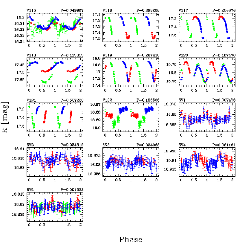
Figure 6: Phased light curves for newly discovered variables. Data from the first night is shown as filled squares, the second night is shown as open circles, and the third night is shown as open triangles. $P$ is the period in days. We do not show data from the first night for the suspected variables when the noise from that night is greater than the amplitude of variability from the last two nights.

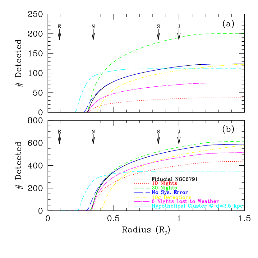
Figure 7: The expected number of hot planets ($P=3-9$ days, a), and very hot planets ($P=1-3$ days, b) detected as a function of planetary radius assuming all stars have planets of the given radius within the stated periods. For the fiducial calculation we assume 20 nights of perfect weather, 7 hours per night, and a detection threshold of $6.5\sigma$.

Table 1: New variable stars identified in the field of NGC 6791. Stars listed as “SV” are suspected variables.

ID	$\alpha_{2000}$	$\delta_{2000}$	Period (days)	R	$A_{R}$
V115	19h20m10$\fs$22	37°43′12$\farcs$2	0.049967	16.21	0.018
V116	19h20m36$\fs$36	37°39′56$\farcs$7	0.393266	17.26	0.357
V117	19h20m51$\fs$00	37°39′03$\farcs$9	0.258878	17.36	0.524
V118	19h21m07$\fs$07	37°54′58$\farcs$9	0.113333	17.48	0.135
V129	19h21m29$\fs$03	37°55′56$\farcs$3	0.267418	16.92	0.594
V120	19h21m43$\fs$46	37°39′56$\farcs$9	0.107470	16.80	0.116
V121	19h21m54$\fs$52	37°40′53$\farcs$4	0.527230	17.30	0.498
V122	19h21m56$\fs$94	37°49′23$\farcs$7	0.186566	16.88	0.020
SV1	19h20m50$\fs$28	37°40′06$\farcs$9	0.007476	16.68	0.003
SV2	19h21m10$\fs$35	37°44′40$\farcs$0	0.034812	16.82	0.005
SV3	19h21m39$\fs$05	37°58′04$\farcs$6	0.034068	16.98	0.005
SV4	19h21m47$\fs$01	37°45′45$\farcs$3	0.081161	16.91	0.007
SV5	19h21m53$\fs$45	37°49′45$\farcs$0	0.004522	16.82	0.005

Note. — Coordinates are from 2MASS where available. The first 8 entries are confirmed variables while the last five are low amplitude suspected variables. The periods listed are those used to phase the light curves in Fig. 6 and should not be treated as a constrained value for the period. Amplitudes are defined as the difference between the third brightest and third faintest observations in the data presented in Fig. 6, while average magnitudes are flux-weighted.

References

- Alard (2000) Alard, C. 2000, A&AS, 144, 363
- Alard & Lupton (1998) Alard, C., & Lupton, R. H. 1998, ApJ, 503, 325
- Bruntt et al. (2003) Bruntt, H., Grundahl, F., Tingley, B., Frandsen, S., Stetson, P. B., & Thomson, B. 2003, A&A, 410, 323
- Butler et al. (2004) Butler, P., et al. 2004, ApJ, 617L, 580
- Chaboyer, Green, & Liebert (1999) Chaboyer, B., Green, E. M., & Liebert, J. 1999, AJ, 117, 1360
- Devor (2005) Devor, J. 2005, ApJ, in press, astro-ph/0504399
- Fischer & Valenti (2005) Fischer, D. A., & Valenti, J. 2005, ApJ, 622, 1102
- Gaudi, Seager, & Mallen-Ornelas (2005) Gaudi, B. S., Seager, S., & Mallen-Ornelas, G. 2005, ApJ, 623, 472
- Gilliland & Brown (1992) Gilliland, R. L, & Brown, T. M. 1992, PASP, 104, 582G
- Gilliland et al. (1993) Gilliland, R. L., et al. 1993, AJ, 106, 2441G
- Gilliland et al. (2000) Gilliland, R. L., et al. 2000, ApJ, 545, 47L
- Girardi et al. (2000) Girardi, L., Bressan, A., Bertelli, G., & Chiosi, C. 2000, A&AS, 141, 371
- Hartman et al. (2004) Hartman, J. D., Bakos, G., Stanek, K. Z., & Noyes, R. W. 2004, AJ, 128, 1761
- Horne (2003) Horne, K. 2003, in ASP Conf. Ser. 294, Scientific Frontiers in Research on Extrasolar Planets, ed. D. Deming & S. Seager (San Francisco: ASP), 361
- Jha et al. (2000) Jha, S., Charbonneau, D., Garnavich, P. M., Sullivan, D. J., Sullivan, T., Brown, T. M., & Tonry, J. L. 2000, ApJ, 540L, 45
- Kaluzny & Udalski (1992) Kaluzny, J., & Udalski, A. 1992, Acta Astronomica, 42, 29
- Kaluzny & Ruciński (1993) Kaluzny, J., & Ruciński, S. M. 1993, MNRAS, 265, 34
- Kjeldsen & Frandsen (1992) Kjeldsen, H., & Frandsen, S. 1992, PASP, 104, 413
- Konacki et al. (2004) Konacki, M., Torres, G., Sasselov, D. D., & Jha, S. 2004, ApJ, in press, astro-ph/0412400
- Kurtz et al. (2005) Kurtz, D. W. 2005, MNRAS, 358, 651
- McArthur et al. (2004) McArthur, B., et al. (2004), ApJ, 614L, 81
- McLeod et al. (2000) McLeod, B. A., Conroy, M., Gauron, T. M., Geary, J. C., & Ordway, M. P. 2000, fdso.conf, 11
- Mochejska et al. (2002) Mochejska, B. J., Stanek, K. Z., Sasselov, D. D., & Szentgyorgyi, A. H. 2002, AJ, 123, 3460M
- Mochejska, Stanek, & Kaluzny (2003) Mochejska, B. J., Stanek, K. Z., & Kaluzny, J. 2003, AJ, 125, 3175
- Mochejska et al. (2005) Mochejska, B. J., et al. 2005, astro-ph/0501145
- Pepper & Gaudi (2005) Pepper, J., & Gaudi, B. S. 2005, astro-ph/0504162
- Pont et al. (2005) Pont, F., et al. 2005, A&AL, in press, astro-ph/0501611
- Ruciński, Kaluzny, & Hilditch (1996) Ruciński, S. M., Kaluzny, J., & Hilditch, R. W. 1996, MNRAS, 282, 705
- Santos et al. (2004) Santos, N., et al. 2004, A&AL, 426, 19
- Santos, Israelian, & Mayor (2004) Santos, N. C, Israelian, G., & Mayor, M. 2004, A&A, 415, 1153
- Schwarzenberg-Czerny (1996) Schwarzenberg-Czerny, A. 1996, ApJ, 460, L107
- Stetson (1987) Stetson, P. B. 1987, PASP, 99, 191
- Stetson (1992) Stetson, P. B. 1992, JRASC, 86, 71
- Udalski et al. (2004) Udalski, A., Pietrzynski, G., Szymanski, M., Kubiak, M., Zebrun, K., Soszynski, I., Szewczyk, K., & Wyrzykowski, L. 2004, Acta Astronomica, 54, 313
- Young (1967) Young, A. T. 1967, AJ, 72, 747
- Young (1993) Young, A. T. 1993, Obs, 113, 41