The Relationship Between Luminosity and Broad-Line Region Size in Active Galactic Nuclei

Abstract

We reinvestigate the relationship between the characteristic broad-line region size ($R_{\rm BLR}$) and the Balmer emission-line, X-ray, UV, and optical continuum luminosities. Our study makes use of the best available determinations of $R_{\rm BLR}$ for a large number of active galactic nuclei (AGNs) from Peterson et al. Using their determinations of $R_{\rm BLR}$ for a large sample of AGNs and two different regression methods, we investigate the robustness of our correlation results as a function of data sub-sample and regression technique. Though small systematic differences were found depending on the method of analysis, our results are generally consistent. Assuming a power-law relation $R_{\rm BLR}$ $\propto L^{\alpha}$, we find the mean best-fitting $\alpha$ is about $0.67\pm 0.05$ for the optical continuum and the broad H$\beta$ luminosity, about $0.56\pm 0.05$ for the UV continuum luminosity, and about $0.70\pm 0.14$ for the X-ray luminosity. We also find an intrinsic scatter of $\sim 40$% in these relations. The disagreement of our results with the theoretical expected slope of 0.5 indicates that the simple assumption of all AGNs having on average same ionization parameter, BLR density, column density, and ionizing spectral energy distribution, is not valid and there is likely some evolution of a few of these characteristics along the luminosity scale.

1. Introduction

There is mounting evidence that massive black holes reside in the centers of most or all massive galaxy bulges. Understanding the demographics and properties of these black holes will hopefully clarify their roles in galaxy formation and evolution, the ionization of the intergalactic medium, and more. The masses of the central black holes in nearby non-active galaxies have been measured using stellar and gas kinematics of the central regions (Tremaine et al. 2002 and references therein). In active galactic nuclei (AGNs), the technique of reverberation mapping (Blandford & McKee 1982; Peterson 1993; Netzer & Peterson 1997) has been used to measure the light-travel-time delay over which broad emission line flux responds to continuum luminosity variations, and to thus deduce the characteristic size of the broad-line region (BLR) around the central, photoionizing source. By assuming the emission lines are broadened primarily by the virial gas motions in the gravitational potential of the central object, the BLR size and the line width then give an estimate of the mass of the central object (Peterson & Wandel 1999).

Wandel et al. (1999) compiled reverberation-based BLR sizes for 17 Seyfert-1 galaxies and derived a scaling relation between BLR size and AGN luminosity. Kaspi et al. (2000) measured reverberation-based BLR sizes for 17 high-luminosity AGNs from the Palomar-Green sample of quasars. Combining these measurements with those of the 17 Seyfert galaxies, Kaspi et al. (2000) found that the BLR size scales with AGN optical luminosity as $R_{\rm BLR}\propto L^{0.70\pm 0.03}$. Assuming that this scaling relation is universal to AGNs of all luminosities and redshifts, several recent studies have used the relation to estimate the central masses in large AGN samples using a single-epoch measurement of the luminosity and the line width (e.g., Wang & Lu 2001; Woo & Urry 2002; Grupe & Mathur 2004). Since the reverberation studies above were based on the Balmer emission lines, generally broad H$\beta$, and on the optical AGN luminosity, single-epoch estimates for objects at redshifts $z\gtrsim 0.6$ have had to rely either on IR observations (e.g., Shemmer et al. 2004) or on attempts to extend the optically based size-luminosity relation to UV luminosities and UV broad emission lines (McLure & Jarvis 2002; Vestergaard 2002). While important progress has been made, there are still a number of potential problems that need to be addressed (e.g., Maoz 2002; Shemmer et al. 2004; Baskin & Laor 2005).

In a recent study, Peterson et al. (2004) compiled all available reverberation mapping data, obtained over the past 15 years, and analyzed them in a uniform and self-consistent way to improve the estimates of the black-hole masses. They find that for a given luminosity, the black-hole mass can be predicted to a precision (random component of the error) of typically about 30%. However, there is also a systematic component of the error, due to the unknown geometry and kinematics of the BLR, that amounts to a factor of about three, based on the scatter in the relationship between black hole mass and bulge velocity dispersion (Onken et al. 2004). In the present paper we use the BLR sizes compiled by Peterson et al. (2004) and study their relationship with the AGN luminosity measured in X-ray, UV, and optical continuum bands and in the broad H$\beta$ emission line. In § 2 we explain how the data were derived, in § 3 we present the relation of the BLR size to the variously defined luminosities, and in § 4 we discuss our results. In § 5 we present a short summary. Unless otherwise noted all wavelength mentioned in this work are common rest-frame wavelengths.

2. Data

Delay times for 35 AGNs with single or multiple data sets were calculated by Peterson et al (2004). For the current study we use the Balmer line time delays, as listed in their Table 6, Column 3 (“rest-frame time lags”). As noted by Kaspi et al. (2000), the derived BLR size from the first three Balmer lines (H$\alpha$, H$\beta$, and H$\gamma$) are consistent with each other and averaging them reduces the scatter in the relation. We have calculated the error-weighted mean BLR size derived from these lines where available. We used only results which were designated by Peterson et al. (2004) as reliable (see their section 4). While we do not necessarily expect each of the Balmer lines to have the same lag, we find empirically that the precision of the lag measurement for any one line is sufficiently low that averaging the Balmer line lags for any particular source reduces the scatter in the radius-luminosity relationship. We find a similar result when we average multiple H$\beta$ lag and optical luminosity measurements for a single source.

Note that in their final mass–luminosity relation Peterson et al. (2004) excluded several data sets for which the full width at half maximum (FWHM) determination was deemed to be unreliable. Since FWHM does not enter the present analysis we have included several of these data sets if their measured time lag was designated as reliable. We have also included an additional data set for NGC 4051 presented by Shemmer et al. (2003). The mean BLR size for each data set is listed in Table 1, Column 3. The described analysis below was done twice – once using the Balmer-line averaged BLR size versus the luminosity, and a second time using only the H$\beta$ BLR sizes. The two analysis sets are discussed in § 3. In the case where only the H$\beta$ BLR sizes were used, 3 objects (PG 0844+349, PG 1211+143, and NGC4593) were excluded, since their H$\beta$-based BLR size measurement is considered unreliable.

In the following subsections we explain how the luminosity at each wavelength band was calculated. We assume a standard cosmology with $H_{0}=70$ km s^-1 Mpc^-1, $\Omega_{M}=0.3$, and $\Omega_{\Lambda}=0.7$. The luminosities are tabulated in Tables 1 and 2 together with the measured fluxes (in the observer’s frame) from which they were derived.

Table 1Optical Observed Fluxes and Luminosities

Object	Ref.	Time lag	$F$(H$\beta$)	$L$(H$\beta$)	$f_{\lambda}$(5100Å)	$\lambda L_{\lambda}$(5100Å)
			$10^{-13}$	$10^{43}$	$10^{-15}$	$10^{44}$
		lt-days	ergs cm-2 s-1	ergs s-1	ergs cm-2 s-1 Å-1	ergs s-1
(1)	(2)	(3)	(4)	(5)	(6)	(7)
Mrk 335	1	$16.8^{+4.8}_{-4.2}$	$7.88\pm 0.36$	$0.1328\pm 0.0060$	$7.68\pm 0.53$	$0.678\pm 0.047$
	1	$12.5^{+6.6}_{-5.5}$	$8.63\pm 0.21$	$0.1455\pm 0.0036$	$8.81\pm 0.47$	$0.777\pm 0.041$
		14.7${}^{+3.0}_{-3.0}$	$\cdots$	0.1392$\pm$ 0.0048	$\cdots$	0.727$\pm$0.044
PG 0026+129	2	$104.7^{+18.3}_{-18.9}$	$1.27\pm 0.11$	$0.8262\pm 0.0698$	$2.69\pm 0.40$	$10.3\pm 1.5$
PG 0052+251	2	$84.4^{+15.3}_{-13.3}$	$1.80\pm 0.21$	$1.3290\pm 0.1567$	$2.07\pm 0.37$	$9.1\pm 1.6$
Fairall 9	3	$17.4^{+3.2}_{-4.3}$	$7.97\pm 0.37$	$0.4494\pm 0.0207$	$5.95\pm 0.66$	$1.79\pm 0.20$
Mrk 590	1	$20.7^{+3.5}_{-2.7}$	$4.41\pm 0.29$	$0.0783\pm 0.0052$	$7.89\pm 0.62$	$0.736\pm 0.058$
	1	$14.0^{+8.5}_{-8.8}$	$2.11\pm 0.71$	$0.0375\pm 0.0126$	$5.33\pm 0.56$	$0.497\pm 0.053$
	1	$29.2^{+4.9}_{-5.0}$	$3.05\pm 0.32$	$0.0542\pm 0.0058$	$6.37\pm 0.45$	$0.594\pm 0.042$
	1	$28.8^{+3.6}_{-4.2}$	$4.44\pm 0.44$	$0.0789\pm 0.0079$	$8.43\pm 1.30$	$0.786\pm 0.122$
		23.2${}^{+7.3}_{-7.3}$	$\cdots$	0.0622$\pm$0.0079	$\cdots$	0.653$\pm$0.069
3C 120	1	$38.1^{+21.3}_{-15.3}$	$3.78\pm 0.37$	$0.2311\pm 0.0227$	$4.30\pm 0.77$	$1.39\pm 0.25$
Akn 120	1	$47.1^{+8.3}_{-12.4}$	$10.64\pm 0.67$	$0.3753\pm 0.0236$	$10.37\pm 0.46$	$1.927\pm 0.086$
	1	$37.1^{+4.8}_{-5.4}$	$7.31\pm 0.83$	$0.2580\pm 0.0294$	$7.82\pm 0.83$	$1.45\pm 0.16$
		42.1${}^{+7.1}_{-7.1}$	$\cdots$	0.3167$\pm$0.0265	$\cdots$	1.69$\pm$0.12
Mrk 79	1	$9.0^{+8.3}_{-7.8}$	$5.38\pm 0.33$	$0.0747\pm 0.0046$	$6.96\pm 0.67$	$0.502\pm 0.048$
	1	$16.1^{+6.6}_{-6.6}$	$5.79\pm 0.48$	$0.0803\pm 0.0067$	$8.49\pm 0.86$	$0.612\pm 0.062$
	1	$16.0^{+6.4}_{-5.8}$	$5.41\pm 0.28$	$0.0750\pm 0.0039$	$7.40\pm 0.72$	$0.534\pm 0.052$
		13.7${}^{+4.1}_{-4.1}$	$\cdots$	0.0767$\pm$0.0051	$\cdots$	0.550$\pm$0.054
PG 0804+761	2	$162.5^{+31.2}_{-31.2}$	$6.45\pm 0.42$	$1.8020\pm 0.1170$	$5.48\pm 1.00$	$8.6\pm 1.6$
PG 0844+349	2	$32.3^{+13.7}_{-13.4}$	$3.02\pm 0.30$	$0.3325\pm 0.0330$	$3.71\pm 0.38$	$2.21\pm 0.23$
Mrk 110	1	$24.3^{+5.5}_{-8.3}$	$4.17\pm 0.17$	$0.1249\pm 0.0049$	$3.45\pm 0.36$	$0.547\pm 0.057$
	1	$20.4^{+10.5}_{-6.3}$	$3.38\pm 0.22$	$0.1011\pm 0.0066$	$3.96\pm 0.51$	$0.628\pm 0.080$
	1	$33.3^{+14.9}_{-10.0}$	$2.99\pm 0.09$	$0.0897\pm 0.0025$	$2.64\pm 0.86$	$0.42\pm 0.14$
		26.0${}^{+6.6}_{-6.6}$	$\cdots$	0.1052$\pm$0.0047	$\cdots$	0.531$\pm$0.091
PG 0953+414	2	$151.1^{+16.9}_{-21.8}$	$1.60\pm 0.09$	$2.6980\pm 0.1571$	$1.56\pm 0.21$	$16.6\pm 2.2$
NGC 3227	5,6	$11.4^{+4.4}_{-6.7}$	$12.53\pm 1.95$	$0.0044\pm 0.0007$	$14.41\pm 2.46$	$0.0256\pm 0.0044$
	7	$5.4^{+14.1}_{-8.7}$	$5.10\pm 0.43$	$0.0018\pm 0.0002$	$12.70\pm 0.68$	$0.0228\pm 0.0012$
		8.4${}^{+4.2}_{-4.2}$	$\cdots$	0.0031$\pm$0.0004	$\cdots$	0.0242$\pm$0.0028
NGC 3516	7,8	$10.9^{+4.4}_{-2.1}$	$10.82\pm 10.23$	$0.0216\pm 0.0025$	$7.83\pm 2.35$	$0.077\pm 0.023$
NGC 3783	9,10	$10.2^{+3.3}_{-2.3}$	$10.13\pm 0.79$	$0.0308\pm 0.0024$	$11.38\pm 0.95$	$0.178\pm 0.015$
NGC 4051	12	$5.8^{+2.6}_{-1.8}$	$5.02\pm 0.51$	$0.0006\pm 0.0001$	$13.38\pm 0.92$	$0.0086\pm 0.0006$
	28	$2.8^{+1.3}_{-1.3}$	$3.09\pm 0.26$	$0.0004\pm 0.0001$	$13.86\pm 0.48$	$0.0089\pm 0.0003$
		4.3${}^{+2.1}_{-2.1}$	$\cdots$	0.0005$\pm$0.0001	$\cdots$	0.0087$\pm$0.0004
NGC 4151	13	$3.1^{+1.1}_{-1.0}$	$72.83\pm 4.66$	$0.0193\pm 0.0012$	$81.67\pm 4.72$	$0.1110\pm 0.0064$
	26	$11.2^{+2.7}_{-2.4}$	$21.6\pm 16.2$	$0.0057\pm 0.0043$	$38.31\pm 2.81$	$0.0519\pm 0.0038$
		7.1${}^{+5.7}_{-5.7}$	$\cdots$	0.0125$\pm$0.0028	$\cdots$	0.0815$\pm$0.0051
PG 1211+143	2	$93.2^{+19.7}_{-29.9}$	$5.45\pm 0.67$	$0.9727\pm 0.1193$	$5.66\pm 0.92$	$5.57\pm 0.90$
PG 1226+023	2	$352.4^{+73.3}_{-73.3}$	$17.22\pm 1.40$	$12.4600\pm 1.0160$	$21.30\pm 2.60$	$91.1\pm 11.1$
PG 1229+204	2	$33.5^{+14.6}_{-12.4}$	$1.98\pm 0.25$	$0.2045\pm 0.0258$	$2.15\pm 0.23$	$1.21\pm 0.13$
NGC 4593	6,14	$3.2^{+5.5}_{-4.1}$	$3.95\pm 1.11$	$0.0077\pm 0.0022$	$12.20\pm 3.90$	$0.122\pm 0.039$
PG 1307+085	2	$111.4^{+32.8}_{-43.2}$	$1.92\pm 0.26$	$1.3720\pm 0.1830$	$1.79\pm 0.18$	$7.54\pm 0.76$
IC 4329A	15	$1.5^{+2.7}_{-1.8}$	$3.05\pm 0.30$	$0.0212\pm 0.0021$	$5.79\pm 0.73$	$0.208\pm 0.026$
Mrk 279	16	$16.7^{+3.9}_{-3.9}$	$5.73\pm 0.40$	$0.1282\pm 0.0089$	$6.90\pm 0.69$	$0.810\pm 0.082$
	25	$12.4^{+9.5}_{-11.9}$	$2.46\pm 0.43$	$0.0550\pm 0.0096$	$5.80\pm 1.95$	$0.68\pm 0.23$
		14.6${}^{+3.0}_{-3.0}$	$\cdots$	0.0916$\pm$0.0093	$\cdots$	0.75$\pm$0.16
PG 1411+442	2	$101.6^{+31.0}_{-28.1}$	$3.33\pm 0.18$	$0.6829\pm 0.0371$	$3.71\pm 0.32$	$4.22\pm 0.36$
NGC 5548	17	$19.7^{+1.5}_{-1.5}$	$8.62\pm 0.85$	$0.0609\pm 0.0060$	$9.92\pm 1.26$	$0.362\pm 0.046$
	17	$18.6^{+2.1}_{-2.3}$	$5.98\pm 1.17$	$0.0422\pm 0.0083$	$7.25\pm 1.00$	$0.26\pm 0.037$
	17	$15.9^{+2.9}_{-2.5}$	$7.46\pm 0.81$	$0.0527\pm 0.0057$	$9.40\pm 0.93$	$0.343\pm 0.034$
	17	$11.0^{+1.9}_{-2.0}$	$4.96\pm 1.44$	$0.0350\pm 0.0102$	$6.72\pm 1.17$	$0.246\pm 0.043$
	17	$13.0^{+1.6}_{-1.4}$	$7.93\pm 0.53$	$0.0560\pm 0.0037$	$9.06\pm 0.86$	$0.331\pm 0.032$
	17	$13.4^{+3.8}_{-4.3}$	$7.58\pm 0.94$	$0.0535\pm 0.0066$	$9.76\pm 1.10$	$0.356\pm 0.040$
	17	$21.7^{+2.6}_{-2.6}$	$9.27\pm 0.70$	$0.0654\pm 0.0050$	$12.09\pm 1.00$	$0.442\pm 0.037$
	17	$16.4^{+1.2}_{-1.1}$	$7.95\pm 0.87$	$0.0561\pm 0.0061$	$10.56\pm 1.64$	$0.386\pm 0.060$
	17	$17.5^{+2.0}_{-1.6}$	$7.41\pm 0.95$	$0.0523\pm 0.0067$	$8.12\pm 0.91$	$0.297\pm 0.033$
	17	$26.5^{+4.3}_{-2.2}$	$10.27\pm 1.04$	$0.0725\pm 0.0073$	$13.47\pm 1.45$	$0.492\pm 0.053$
	17	$24.8^{+3.2}_{-3.0}$	$9.34\pm 0.61$	$0.0659\pm 0.0043$	$11.83\pm 1.82$	$0.432\pm 0.066$
	17	$6.5^{+5.7}_{-3.7}$	$6.27\pm 1.22$	$0.0443\pm 0.0086$	$6.98\pm 1.20$	$0.255\pm 0.044$

Table 1— $Continued$

Object	Ref.	Time lag	$F$(H$\beta$)	$L$(H$\beta$)	$f_{\lambda}$(5100Å)	$\lambda L_{\lambda}$(5100Å)
			$10^{-13}$	$10^{43}$	$10^{-15}$	$10^{44}$
		lt-days	ergs cm-2 s-1	ergs s-1	ergs cm-2 s-1 Å-1	ergs s-1
(1)	(2)	(3)	(4)	(5)	(6)	(7)
	17	$14.3^{+5.9}_{-7.3}$	$5.26\pm 1.12$	$0.0372\pm 0.0079$	$7.03\pm 0.86$	$0.257\pm 0.032$
	27	$7.6^{+4.8}_{-4.0}$	$7.10\pm 0.60$	$0.0501\pm 0.0042$	$5.78\pm 0.62$	$0.211\pm 0.023$
		16.2${}^{+5.9}_{-5.9}$	$\cdots$	0.0532$\pm$0.0065	$\cdots$	0.334$\pm$0.041
PG 1426+015	2	$84.7^{+21.4}_{-24.4}$	$3.09\pm 0.28$	$0.6302\pm 0.0581$	$4.62\pm 0.71$	$5.21\pm 0.80$
Mrk 817	1	$19.0^{+3.9}_{-3.7}$	$4.73\pm 0.26$	$0.1100\pm 0.0061$	$6.10\pm 0.83$	$0.75\pm 0.10$
	1	$15.3^{+3.7}_{-3.5}$	$4.00\pm 0.40$	$0.0930\pm 0.0092$	$5.00\pm 0.49$	$0.61\pm 0.06$
	1	$33.6^{+6.5}_{-7.6}$	$3.38\pm 0.19$	$0.0785\pm 0.0045$	$5.01\pm 0.27$	$0.612\pm 0.033$
		22.6${}^{+9.7}_{-9.7}$	$\cdots$	0.0938$\pm$0.0066	$\cdots$	0.656$\pm$0.065
PG 1613+658	2	$40.1^{+15.0}_{-15.2}$	$2.02\pm 0.13$	$0.9496\pm 0.0632$	$3.49\pm 0.43$	$9.5\pm 1.2$
PG 1617+175	2	$86.8^{+16.0}_{-20.2}$	$1.40\pm 0.17$	$0.5123\pm 0.0636$	$1.44\pm 0.25$	$3.00\pm 0.52$
PG 1700+518	2	$251.8^{+45.9}_{-38.8}$	$1.89\pm 0.10$	$5.5520\pm 0.2882$	$2.20\pm 0.15$	$42.34\pm 2.89$
3C 390.3	21	$23.6^{+6.2}_{-6.7}$	$2.12\pm 0.17$	$0.1950\pm 0.0153$	$1.73\pm 0.28$	$0.87\pm 0.14$
Mrk 509	1	$79.6^{+6.1}_{-5.4}$	$12.30\pm 0.06$	$0.3985\pm 0.0020$	$10.92\pm 1.99$	$1.88\pm 0.34$
PG 2130+099	2	$177.1^{+19.9}_{-12.7}$	$5.12\pm 0.46$	$0.5558\pm 0.0498$	$4.84\pm 0.45$	$2.85\pm 0.26$
NGC 7469	23	$4.5^{+0.6}_{-0.7}$	$7.80\pm 0.35$	$0.0577\pm 0.0026$	$13.57\pm 0.61$	$0.521\pm 0.023$

Note. — Bold font lines give average values for objects with multiple data sets. The mean time lag is computed as a simple mean and its uncertainty is the rms of the individual measurements. The mean luminosity is computed as a simple mean and its uncertainty is the simple mean of the individual uncertainties (which are derived from the rms of each light curve).

Table 2Object Characteristics

Object	Redshift	$E(B-V)$	$f_{\lambda}$(1450Å)	$\lambda L_{\lambda}$(1450Å)	$F$(2–10 keV)	$L$(2–10 keV)	Ref.	$F$(H$\beta_{\rm narrow}$)
			$10^{-14}$	$10^{44}$	$10^{-12}$	$10^{43}$		$10^{-13}$
			ergs cm-2 s-1 Å-1	ergs s-1	ergs cm-2 s-1	ergs s-1		ergs cm-2 s-1
(1)	(2)	(3)	(4)	(5)	(6)	(7)	(8)	(9)
Mrk 335	0.02578	0.035	$7.2\pm 1.0$	$2.12\pm 0.30$	$9.43\pm 0.10$	$1.430\pm 0.015$	1	0.410
PG 0026+129	0.14200	0.071	$1.5\pm 0.5$	$22.36\pm 7.45$	$6.33\pm 0.13$	$34.16\pm 0.70$	3	0.063
PG 0052+251	0.15500	0.047	$1.1\pm 0.2$	$16.88\pm 3.07$	$10.09\pm 0.17$	$66.0\pm 1.1$	3	0.091
Fairall 9	0.04702	0.027	$3.5\pm 1.0$	$3.38\pm 0.97$	$19.06\pm 1.00$	$9.92\pm 0.52$	2	0.283
Mrk 590	0.02638	0.037	$2.4\pm 1.4$	$0.75\pm 0.44$	$27.00\pm 2.70$	$4.29\pm 0.43$	7	0.121
3C 120	0.03301	0.297	$1.2\pm 1.2$	$4.45\pm 4.23$	$44.28\pm 2.22$	$11.13\pm 0.56$	2	0.151
Akn 120	0.03230	0.128	$3.5\pm 0.5$	$3.34\pm 0.48$	$27.34\pm 2.73$	$6.57\pm 0.66$	5	0.364
Mrk 79	0.02219	0.071	$2.0\pm 1.0$	$0.57\pm 0.29$	$25.96\pm 2.60$	$2.90\pm 0.29$	7	0.221
PG 0804+761	0.10000	0.035	$7.0\pm 1.0$	$36.56\pm 5.22$	$8.34\pm 0.07$	$21.13\pm 0.18$	1	0.
PG 0844+349	0.06400	0.037	$1.7\pm 0.5$	$3.41\pm 1.00$	$2.37\pm 0.02$	$2.34\pm 0.020$	1	0.
Mrk 110	0.03529	0.013	$1.0\pm 0.5$	$0.48\pm 0.24$	$26.64\pm 0.19$	$7.676\pm 0.055$	1	0.148
PG 0953+414	0.23410	0.013	$2.0\pm 1.0$	$64.3\pm 32.1$	$2.58\pm 0.04$	$42.22\pm 0.65$	2	0.534
NGC 3227	0.00386	0.023	$0.04\pm 0.01$	$0.0003\pm 0.0001$	$25.52\pm 1.30$	$0.0839\pm 0.0043$	2	0.558
NGC 3516	0.00884	0.042	$3.0\pm 1.5$	$0.106\pm 0.053$	$73.68\pm 3.70$	$1.280\pm 0.064$	2	0.
NGC 3783	0.00973	0.119	$4.8\pm 1.0$	$0.373\pm 0.078$	$51.49\pm 2.55$	$1.085\pm 0.054$	2	0.656
NGC 4051	0.00234	0.013	$1.2\pm 0.2$	$0.0023\pm 0.0004$	$21.21\pm 1.10$	$0.026\pm 0.0013$	2	0.
NGC 4151	0.00332	0.028	$35.\pm 15.$	$0.154\pm 0.066$	$201.\pm 10.$	$0.490\pm 0.025$	2	9.912
PG 1211+143	0.08090	0.035	$3.0\pm 1.0$	$9.8\pm 3.3$	$2.82\pm 0.04$	$4.557\pm 0.065$	1	0.
PG 1226+023	0.15834	0.021	$15.0\pm 4.0$	$200.6\pm 53.5$	$90.33\pm 20.8$	$619.\pm 142.$	3	0.
PG 1229+204	0.06301	0.027	$2.0\pm 1.0$	$3.6\pm 1.8$	$2.54\pm 0.16$	$2.43\pm 0.15$	3	0.152
NGC 4593	0.00900	0.025	$2.0\pm 1.0$	$0.064\pm 0.032$	$31.89\pm 1.60$	$0.575\pm 0.029$	2	0.217
PG 1307+085	0.15500	0.034	$0.8\pm 0.2$	$11.2\pm 2.8$	$3.65\pm 0.35$	$23.9\pm 2.3$	6	0.155
IC 4329A	0.01605	0.059	$\cdots$	$\cdots$	$77.46\pm 3.90$	$4.49\pm 0.23$	2	0.253
Mrk 279	0.03045	0.016	$0.6\pm 0.5$	$0.22\pm 0.18$	$25.92\pm 2.59$	$5.52\pm 0.55$	5	0.325
PG 1411+442	0.08960	0.008	$1.4\pm 0.4$	$4.70\pm 1.34$	$0.78\pm 0.09$	$1.57\pm 0.18$	1	0.140
NGC 5548	0.01717	0.020	$3.0\pm 1.0$	$0.34\pm 0.11$	$46.05\pm 2.30$	$3.06\pm 0.15$	2	0.614
PG 1426+015	0.08647	0.032	$7.5\pm 2.0$	$27.82\pm 7.42$	$5.25\pm 0.25$	$9.77\pm 0.47$	3	0.072
Mrk 817	0.03145	0.007	$1.5\pm 1.0$	$0.54\pm 0.36$	$\cdots$	$\cdots$	$\cdots$	0.078
PG 1613+658	0.12900	0.027	$3.5\pm 1.0$	$30.52\pm 8.72$	$6.14\pm 0.09$	$26.90\pm 0.39$	3	0.041
PG 1617+175	0.11244	0.042	$0.75\pm 0.35$	$5.35\pm 2.50$	$\cdots$	$\cdots$	$\cdots$	0.
PG 1700+518	0.29200	0.035	$0.6\pm 0.4$	$39.4\pm 26.3$	$\cdots$	$\cdots$	$\cdots$	0.
3C 390.3	0.05610	0.071	$0.6\pm 0.2$	$1.17\pm 0.39$	$22.80\pm 5.00$	$17.11\pm 3.75$	4	0.172
Mrk 509	0.03440	0.057	$5.5\pm 1.0$	$3.48\pm 0.63$	$43.10\pm 2.10$	$11.79\pm 0.57$	2	0.777
PG 2130+099	0.06298	0.044	$2.2\pm 0.2$	$4.50\pm 0.41$	$4.80\pm 0.12$	$4.59\pm 0.11$	3	0.385
NGC 7469	0.01632	0.069	$3.0\pm 0.5$	$0.451\pm 0.075$	$27.64\pm 3.40$	$1.66\pm 0.20$	8	1.357

References. — For column 8: 1 - George et al. (2000); 2 - George et al. (1998); 3 - Lawson & Turner (1997); 4 - Leighly et al. (1997); 5 - The Tartarus Database (http://tartarus.gsfc.nasa.gov/); 6 - Williams et al. (1992); 7 - Turner & Pounds (1989); 8 - Nandra et al. (1998).

2.1. General Considerations for the Multiwavelength Datasets

We derived optical luminosities directly from the data sets from which the time lags were measured. Hence, the measurement of the time lag and the optical luminosity is simultaneous. However, the UV and X-ray fluxes were measured simultaneously with the BLR size for only a few AGNs. In these objects, we used these simultaneous UV and X-ray data in the analysis below (UV – NGC 3783, NGC 5548, NGC 4151, 3C390.3, NGC7469, Fairall 9; X-ray – NGC4151, NGC7469). Luminosities were not corrected for host galaxy contribution. To subtract this contribution, a knowledge of the spatial distribution of the host-galaxy luminosity is needed, combined with the slit width and seeing in which the observation was done. This task is beyond the scope of the current paper. However, we note that this correction would be negligible for the quasars in the sample ($\lambda L_{\lambda}$(5100Å)$\gtrsim 10^{44}$ ergs s^-1) and it is likely small for Seyferts as well (e.g., Peterson et al. 1995; Kaspi et al. 1996). Since there might be a systematic effect of greater host-galaxy luminosity contribution in lower luminosity objects, such a correction will tend to flatten the BLR-size – luminosity relation causing the power-law slope to be smaller.

Recent studies (e.g., Gaskell et al. 2004; Hopkins et al. 2004) indicate AGNs have reddening in addition to the Galactic reddening, probably due to gas in their host galaxy or the intergalactic medium. This is affecting the measured luminosity of the AGNs, though it is difficult to determine the intrinsic reddening of individual objects. Hence, we do not attempt to correct for such reddening in the study presented here.

AGNs vary with differing amplitudes and timescales at different wavelengths. Specifically, amplitudes become larger and timescales shorter as one progresses from the rest-frame optical, through the UV, to X-rays (e.g., Edelson et al. 1996). Therefore, another basic limitation of the comparison we make of the size-luminosity relation for luminosities in different bands, beyond the fact that the actual sampling window in each band is very different (e.g., robust median luminosities in the optical, based on tens of epochs, compared with few- or single-epoch-based luminosities in UV and X-rays), is the different statistical properties of the variability within each band.

Table 1 lists all multiple data sets. One line per object (in bold font) gives the mean of all the data sets for this object (cases in which there is only one data set appear with a normal font). This mean will be further discussed in § 3.

2.2. Optical luminosities

Optical luminosities were calculated from the mean 5100 Å flux density of each data set. These luminosities are the same as the ones in Peterson et al. (2004; see their § 8), but with an improved correction for Galactic absorption. We used the $E(B-V)$ values listed in the NASA/IPAC Extragalactic Database (NED) which are taken from Schlegel et al. (1998) and the extinction curve of Cardelli et al. (1989), adjusted to $A_{V}/E(B-V)=3.1$. For most objects the difference in luminosities between the current work and Peterson et al. (2004) is less than 1%, while for a few it reaches up to 7%. The measured 5100 Å flux densities and luminosities are listed in Table 1, Columns 6 and 7, respectively. The luminosity uncertainty is determined as the rms of the light curve of each data set.

We have computed the H$\beta$ luminosity from the average H$\beta$ flux of each data set, correcting the fluxes for Galactic absorption as above. The H$\beta$ flux and luminosity are listed in Table 1, Columns 4 and 5, respectively. We have also estimated the H$\beta$ luminosity with the narrow component removed from the line profile (these narrow-line corrected H$\beta$ fluxes and luminosities do not appear in Table 1). The contribution of the narrow component of H$\beta$ was calculated using the H$\beta$(narrow component)/[O III]$\lambda$5007 line ratio from Marziani et al. (2003), multiplied by the [O III]$\lambda$5007 line flux we measured in the data sets in hand. We used our own estimates for the narrow component of H$\beta$ for: a) AGNs which are not in the Marziani et al. sample (NGC 3227, NGC 4151); b) AGNs which were observed at a low-state and for which we have a particularly good estimate of the narrow component of H$\beta$ (Mrk 79, PG 1229+204, NGC 5548, PG 1426+015). We also did not use the Marziani et al. estimates for five objects (PG 0804+761, PG 0844+349, PG 1211+143, PG 1226+023, PG 1617+175) for which we think their [O III]$\lambda$5007 line fluxes are overestimated due to blending with Fe II$\lambda$5018. The H$\beta$ narrow component line flux we use in our analysis is listed in Table 2, Column 9.

2.3. UV luminosity

For the UV luminosity, we have used both the 1350 Å (used by Vestergaard 2002) and 1450 Å (used by Shemmer et al. 2004) wavelength ranges. UV fluxes at these rest frame wavelengths were measured, for most objects, using FOS and STIS spectra taken from the Hubble Space Telescope (HST) archive. In cases where multiple observations exist, we have used the averaged flux density, except for the few cases where the UV data were obtained simultaneously with the optical time lag measurements – see § 2. In several cases (Mrk 110, PG 1229+204, PG 1426+015, Mrk 817, PG 1613+658) there were no observations at 1350 Å or 1450 Å but spectra at about 1200 Å could be extrapolated (using a straight line) in order to estimate the 1350 Å and 1450 Å flux densities. For several objects without HST UV spectra we used archival International Ultraviolet Explorer (IUE) spectra to measure the 1350 Å and 1450 Å flux densities. These objects are 3C 120, Mrk 590, Mrk 79, and PG 1617+175. For one object, IC 4329A, no useful UV data were found. The flux densities were corrected for Galactic absorption, as described above for the 5100 Å flux density. The measured 1450 Å flux densities and calculated luminosities are listed in Table 2 in Columns 4 and 5, respectively.

2.4. X-ray luminosity

Most of the objects with reverberation mapping data also have X-ray data in the literature and in archives. We searched the literature for the 2–10 keV fluxes of each object (see references in Table 2, column 8). For 3 objects (PG 1700+519, Mrk 817, and PG 1617+175), no useful X-ray data were found. The fluxes were corrected for Galactic absorption using the PIMMS tool (Mukai 1993) and the published power-law slopes and Galactic column densities. The observed 2–10 keV band was K-corrected to yield the rest-frame 2–10 keV luminosity. We note, however, that because of the small Galactic absorption of most objects and their small redshifts, these corrections are small (of order of a few percent and hence much smaller than the known X-ray variability). Also, any intrinsic absorption has a negligible effect in this hard X-ray energy range. The measured fluxes in the observed 2–10 keV band and the calculated luminosities in the rest-frame 2–10 keV band are listed in Table 2 Columns 6 and 7, respectively.

3. BLR Size – Luminosity Relations

The relations between the BLR size and the various luminosities described above are plotted in Figure 1. The power-law relation between the BLR size and $\lambda L_{\lambda}$(5100 Å) is clearly confirmed by our analysis. Such a relation is also apparent when UV, X-ray, and H$\beta$ luminosities are used. Two obvious outliers, which do not fit the general trends in any of the wavelength bands, are NGC 3227 and NGC 4051. These are the two-least luminous objects in all wavelength bands. This behavior could be due to major reddening or obscuration in these two objects, which decreases their measured luminosity (e.g., NGC 3227 - Crenshaw et al. 2001; NGC 4051 - Kaspi et al. 2004). For NGC 3227, the extinction correction suggested by Crenshaw et al. (2001) increases the UV luminosity (at 1450 Å) by a factor of $\sim 66$ and the optical luminosity by a factor of $\sim 2$ (see Figure 1). Although this would improve the agreement of this data point with the general trend, it would still remain an outlier. An alternative explanation can be that the BLR-size – luminosity relation found at high luminosities breaks down at low luminosities. We will exclude these two objects from our fits to the BLR-size – luminosity relation, noting the derived relation applies to AGNs with optical luminosity in the range $10^{43}<\lambda L_{\lambda}(5100{\rm\AA})<10^{46}$ ergs s^-1.

Figure 1.— Balmer-line averaged BLR size plotted versus various luminosities given in ergs s^-1. The left side panels show all data sets and the right side panels show one averaged data set per object. The data are listed in Tables 1 and 2. For each panel two fits (excluding the two lowest luminosity objects) are shown: solid line – FITEXY and dashed line - BCES. Fits parameters are given in the upper part of Table 3. Right pointing arrows show the shift in location of the data points of NGC 3227 when the Crenshaw et al. (2001) extinction correction is applied.

We have used two methods to calculate the relations between the BLR size and the various luminosities:

1. The linear regression method of Press et al. (1992), in which a straight-line is fitted to the data with errors in both coordinates (known as FITEXY). This method is based on an iterative process to minimize $\chi^{2}$. We follow Tremaine et al. (2002), who account for the intrinsic scatter in the relation by increasing the uncertainties until obtaining $\chi^{2}$ per degree of freedom equal to 1 (see below in Table 3 column 5).

2. The bivariate correlated errors and intrinsic scatter (BCES) regression method of Akritas & Bershady (1996). This method takes into account the uncertainty in both coordinates as well as the intrinsic scatter around a straight line. In our analysis, we use the BCES bisector result which is the mean of the two fits: one when fitting Y as dependent on X, and the other when fitting X as dependent on Y.

Tremaine et al. (2002) compare the two methods using Monte-Carlo simulations and concluded that the FITEXY is superior to the BCES method. However, in their implementation for the BCES method Tremaine et al. (2002) did not use the BCES bisector value. They only used the fit of Y as dependent on X. This might have distorted their conclusion when comparing the two methods. Thus in the analysis below we use both methods. One advantage of the BCES method over the simple FITEXY method is its ability to account for real intrinsic scatter, if it exists in the data. However, the available code of the BCES method does not give any quantification of this scatter. The implementation of the FITEXY method that we use (of Tremaine et al. 2002) also considers intrinsic scatter and allows us to quantify it. Such intrinsic scatter was assumed in previous investigations of the BLR-size – luminosity relation (e.g., Vestergaard 2002), but not quantified.

The two fitting methods do not account for asymmetric uncertainties (e.g., as we have for the uncertainties of the BLR sizes). In order to account for the asymmetric uncertainties, we used in our fits the uncertainty value in the direction of the fitted line. This typically required a few iterations to converge completely.

The correlation analysis below is done in two ways: (1) by using all data sets that are available, where in case of multiple data sets for the same object we treat each data set as independent; (2) by computing the mean BLR size and mean luminosity of all the multiple data sets of the same object, and using only that mean for each object.

In Table 3, we summarize the results from the different fits we carried out for the relation of the various luminosities with the BLR size. For each of the luminosities measured, two lines are given: the first line lists the results when using all data sets and the second line lists the results when using the averaged data set per object. The number of data sets used in the fit is listed in Column 2. The relations are given in the form:

$$\frac{R_{BLR}}{10{\rm\ lt\,days}}=AL^{B}$$ (1)

where $L$ is the luminosity normalized as given in column 1 of Table 3. The parameters A and B are given in columns 3 and 4 for the FITEXY method and in columns 6 and 7 for the BCES method. In column 5 we list the intrinsic scatter, in percent of the value, found when using the FITEXY method. Also, in columns 8 and 9 we list the Pearson and Spearman correlation coefficients, respectively.

As explained in § 2, the analysis was done twice – once using the mean Balmer-line BLR size versus the luminosity (results are presented in the upper part of Table 3), and a second time using only the H$\beta$ BLR sizes (lower part of Table 3). The results from the two analysis sets are consistent and no significant differences are detected. The correlations coefficients (columns 8 and 9 of Table 3) are somewhat higher when using the mean Balmer-line BLR size and this may indicate that using these lags reduces the scatter in the relation with the luminosity. Thus, in the analysis below we refer only to the upper part of Table 3 which uses the mean Balmer-lines time lags.

The results of Table 3 indicate that there is a systematic difference between the two fitting methods. The BCES method slope parameter (B) is generally larger than the one found with the FITEXY fit, and also the constant parameter (A) is generally larger. This illustrates the important issue of how the regression method may influence the correlation results; using different regression methods yields different regression slopes. We could not find what is the main cause for the differences and we attribute them to the different algorithms, strategies, and statistical concepts each of the two methods uses. The real uncertainty of the slope measurement should be the range between the different methods and not necessarily the formal error given by each method. Furthermore, the regression methods are sensitive also to outlier points. We find that the BCES method is much more sensitive to the inclusion or exclusion of the two lower-luminosity points (NGC 3227 and NGC 4051) compared to FITEXY.

In its present implementation the FITEXY method establishes that intrinsic scatter does exist in the BLR size – luminosity relation. Only when we artificially increase the formal measured uncertainty in the BLR size do we find a $\chi^{2}$ of unity. We find that the intrinsic scatter in the relation is $\sim 40$% (Table 3 Column 5). We note that this intrinsic scatter can be caused by a real scatter in the physical BLR size – luminosity relation but also by some systematic effects such as intrinsic reddening, contributions by the host galaxy, or effects of variability due to non-contemporaneous observations. There is currently no way to distinguish between the different contributors to this scatter.

Table 3BLR size — Luminosity relation

Luminosity	N	AFITEXY	BFITEXY	Scatter	ABCES	BBCES	Pearson	Spearman
(1)	(2)	(3)	(4)	(5)	(6)	(7)	(8)	(9)
Using mean Balmer-lines time lag
$L$(H$\beta$)/1043	59	$7.83^{+0.87}_{-0.78}$	$0.619\pm 0.045$	38	$9.42^{+0.93}_{-0.85}$	$0.670\pm 0.050$	0.885	0.860
	33	$7.55^{+0.90}_{-0.81}$	$0.687\pm 0.058$	40	$8.91^{+0.92}_{-0.83}$	$0.690\pm 0.068$	0.916	0.933
$L$(H$\beta$)/1043 no narrow	59	$8.14^{+0.91}_{-0.82}$	$0.618\pm 0.044$	38	$9.68^{+0.99}_{-0.90}$	$0.659\pm 0.052$	0.879	0.872
	33	$7.87^{+0.89}_{-0.80}$	$0.683\pm 0.055$	40	$9.25^{+0.99}_{-0.89}$	$0.686\pm 0.064$	0.916	0.933
$\lambda L_{\lambda}$(5100)/1044	59	$2.45^{+0.18}_{-0.17}$	$0.608\pm 0.045$	40	$2.65^{+0.19}_{-0.18}$	$0.694\pm 0.056$	0.869	0.845
	33	$2.07^{+0.26}_{-0.23}$	$0.665\pm 0.065$	46	$2.39^{+0.32}_{-0.28}$	$0.723\pm 0.075$	0.884	0.910
$\lambda L_{\lambda}$(1450)/1044	58	$2.12^{+0.17}_{-0.15}$	$0.496\pm 0.042$	41	$2.27^{+0.17}_{-0.16}$	$0.595\pm 0.046$	0.865	0.807
	32	$1.76^{+0.26}_{-0.23}$	$0.545\pm 0.063$	45	$2.01^{+0.24}_{-0.21}$	$0.604\pm 0.053$	0.888	0.910
$\lambda L_{\lambda}$(1350)/1044	58	$2.08^{+0.17}_{-0.16}$	$0.499\pm 0.040$	41	$2.25^{+0.17}_{-0.16}$	$0.595\pm 0.046$	0.862	0.803
	32	$1.75^{+0.26}_{-0.22}$	$0.540\pm 0.056$	46	$2.07^{+0.23}_{-0.21}$	$0.584\pm 0.046$	0.887	0.897
$L$(2–10 keV)/1043	54	$0.75^{+0.11}_{-0.10}$	$0.614\pm 0.064$	52	$0.65^{+0.13}_{-0.11}$	$0.830\pm 0.102$	0.705	0.669
	30	$0.86^{+0.18}_{-0.15}$	$0.544\pm 0.091$	64	$0.71^{+0.24}_{-0.18}$	$0.813\pm 0.119$	0.688	0.701
Using only H$\beta$ time lag
$L$(H$\beta$)/1043	55	$7.55^{+0.91}_{-0.82}$	$0.609\pm 0.048$	38	$9.42^{+1.02}_{-0.92}$	$0.669\pm 0.056$	0.874	0.845
	30	$7.18^{+0.94}_{-0.83}$	$0.694\pm 0.064$	40	$8.79^{+1.00}_{-0.90}$	$0.691\pm 0.080$	0.906	0.923
$L$(H$\beta$)/1043 no narrow	55	$7.85^{+0.94}_{-0.84}$	$0.604\pm 0.047$	38	$9.73^{+1.10}_{-0.99}$	$0.657\pm 0.059$	0.867	0.854
	30	$7.49^{+0.99}_{-0.88}$	$0.687\pm 0.063$	40	$9.18^{+1.09}_{-0.98}$	$0.685\pm 0.081$	0.906	0.925
$\lambda L_{\lambda}$(5100)/1044	55	$2.43^{+0.18}_{-0.17}$	$0.601\pm 0.047$	39	$2.69^{+0.20}_{-0.18}$	$0.670\pm 0.060$	0.870	0.843
	30	$2.00^{+0.28}_{-0.24}$	$0.665\pm 0.069$	44	$2.47^{+0.36}_{-0.32}$	$0.674\pm 0.089$	0.882	0.911
$\lambda L_{\lambda}$(1450)/1044	54	$2.11^{+0.17}_{-0.16}$	$0.498\pm 0.044$	39	$2.28^{+0.17}_{-0.16}$	$0.566\pm 0.047$	0.858	0.780
	29	$1.72^{+0.29}_{-0.24}$	$0.548\pm 0.061$	44	$2.13^{+0.29}_{-0.26}$	$0.552\pm 0.062$	0.878	0.894
$\lambda L_{\lambda}$(1350)/1044	54	$2.06^{+0.18}_{-0.16}$	$0.495\pm 0.041$	40	$2.26^{+0.17}_{-0.16}$	$0.557\pm 0.045$	0.854	0.776
	29	$1.72^{+0.27}_{-0.23}$	$0.536\pm 0.058$	44	$2.14^{+0.27}_{-0.24}$	$0.548\pm 0.050$	0.876	0.878
$L$(2–10 keV)/1043	50	$0.74^{+0.11}_{-0.10}$	$0.612\pm 0.063$	48	$0.65^{+0.15}_{-0.12}$	$0.806\pm 0.108$	0.700	0.690
	27	$0.86^{+0.18}_{-0.15}$	$0.532\pm 0.090$	62	$0.71^{+0.31}_{-0.22}$	$0.773\pm 0.139$	0.668	0.695

Note. — For each luminosity in column 1 two rows are given: first row is the fit results where multiple data sets were used for each object, and the second row is the fit results where all data sets per object were averaged. See text for details.

In Figure 2 we plot the mean Balmer-line BLR size versus the $\lambda L_{\lambda}$(5100 Å) luminosity, with one averaged point per object. We also plot four fits: using all 35 points, excluding the low luminosity AGNs, and with the two fitting methods. Within the luminosity range of the measurements ($10^{43}$–$10^{46}$ ergs s^-1) all fits are consistent with each other and all are well within the scatter of the points in the plot. Also, when using only the data for the more luminous ($\gtrsim 5.2\times 10^{43}$) objects (26 objects) from Figure 2, we find a slope of B${}_{\rm FITEXY}=0.63\pm 0.07$ and a constant of A${}_{\rm FITEXY}=2.4\pm 0.3$, which are consistent with the results when using the whole sample.

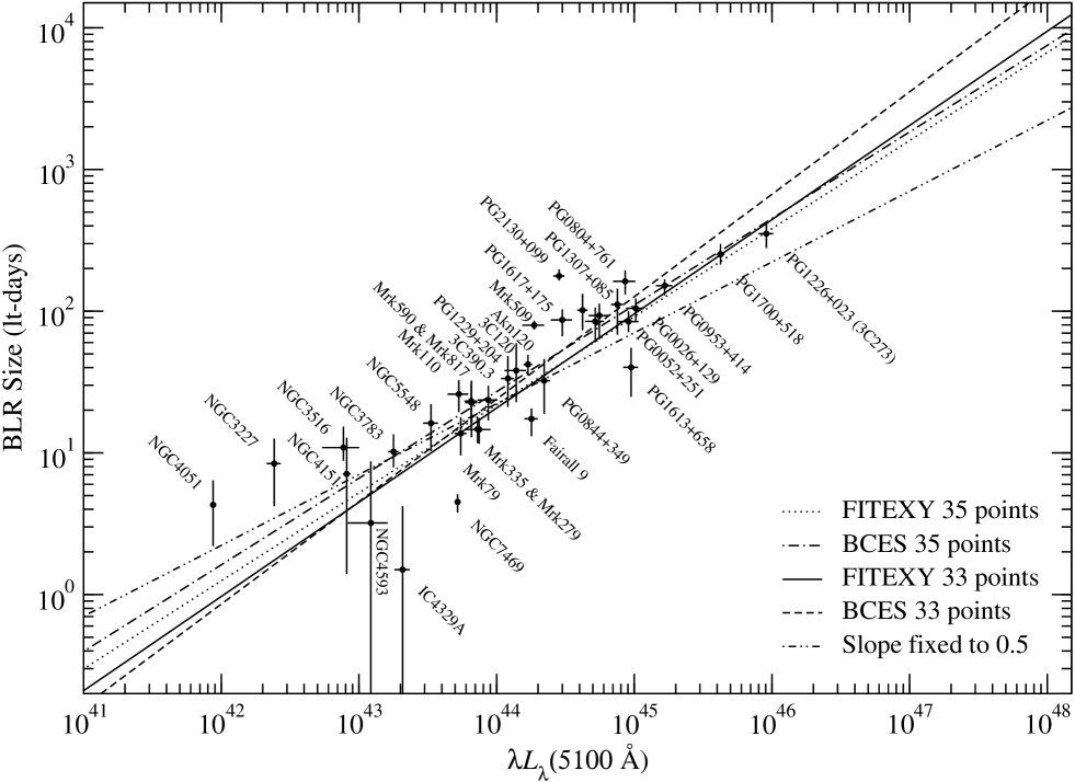
Figure 2.— Balmer-line averaged BLR size plotted versus the $\lambda L_{\lambda}$(5100 Å) luminosity (in units of ergs s^-1) on a larger scale. The BLR size of each data set is determined from the averaged Balmer-line time lags. Objects with multiple data sets have been averaged to one point per object. Five line fits are shown: dotted line - FITEXY using all 35 points; dot-dashed line - BCES using all 35 points; solid line - FITEXY excluding the 2 lower luminosity points; dashed line - BCES excluding the 2 lower luminosity points; dot-dot-dashed line - FITEXY excluding the 2 lower luminosity points and fixing the slope to 0.5.

Comparing the two methods of analysis, using all data sets versus using only one averaged data set per object, we find that the slope parameter (B) is somewhat different while the normalization parameter (A) is similar (both for the BCES and FITEXY methods). In general, when using one averaged data point per object, the slopes are larger by $\sim 0.05$ (which is within the formal uncertainty) than when using all data sets. An argument for using one averaged data point per object is that we do not know if the BLR-size – luminosity relation in a given object is the same as between different objects (the physical processes driving the relation in a single AGN might be different from the ones driving it in a range of objects). Thus, in order to have a relation that spans a large range of luminosity and different objects and to study the physics across the luminosity function, it is better to use the relation with a mean BLR-size and a mean luminosity for each object. On the other hand, if the relation in one object is the same as between objects there is justification to use all data sets. This has been tested observationally for only one object, NGC 5548, by Peterson et al. (2002) who found the BLR-size – luminosity relation has a slope of 0.95 when using optical luminosity and 0.53 for the UV luminosity. While the slope with the UV luminosity is similar to the one we find in Table 3, the optical luminosity slope is not. Hence, it is still not clear if the relation in a single object is the same as in a sample of objects and we present both results in the current study.

Removal of the H$\beta$ narrow component from the total H$\beta$ luminosity affects the fit results only at the 1% level with no obvious general trend. Also, when correlating the BLR size with the UV luminosity, the difference between using the 1350 Å or the 1450 Å bands is negligible (less than 2% and well within the uncertainties), as expected. The flux densities in these bands are very similar, and in some cases identical.

Wu et al. (2004) correlated the BLR size with the H$\beta$ luminosity for the objects of Kaspi et al. (2000) using the data given there. The H$\beta$ luminosity can be considered a good indicator for the AGN luminosity as the line is driven by the ionizing continuum. It was noted by Kaspi et al. (2000) that the use of the H$\beta$ luminosity instead of the optical luminosity do not change their correlation results (see their §4.2). Wu et al. (2004) use only one data set per object and assume a different cosmology ($H_{0}=75$ km s^-1 Mpc^-1 and q${}_{0}=0.5$) and obtain a slope of $0.68\pm 0.11$. This result is consistent with the one we obtain in our analysis (Table 3).

4. What Determines the BLR Size?

A theoretical slope for the relation between the BLR size and the luminosity, predicted by various early papers, is 0.5. This is based on the assumption that, on average, all AGNs have the same ionization parameter, BLR density, column density, and ionizing spectral energy distribution (SED). A slope of 0.5 is also expected if the BLR size is determined by the dust sublimation radius (Netzer & Laor 1993). However, several studies have indicated that the SED is luminosity dependent, and thus at least part of the assumptions above are not justified (e.g., Mushotzky & Wandel 1989; Zheng & Malkan 1993; Puchnarewicz et al. 1996). Here we use the observed relations of the BLR size with the different luminosity bands to study which band influences the BLR size the most.

4.1. UV vs. Optical Continuum Luminosity

Use of the H$\beta$ and $\lambda L_{\lambda}$(5100 Å) luminosities in the BLR-size – luminosity relation yields similar slopes of about 0.69. The slope with the UV luminosity [both $\lambda L_{\lambda}$(1450Å) and $\lambda L_{\lambda}$(1350Å)] is lower by about 0.1 than the slopes using the optical bands (this is manifested both in the FITEXY method and the BCES method). The UV-based slope is the closest to the theoretical expectation of 0.5 based on the assumptions mentioned above.

The UV band (i.e., 1200–3000 Å) is close in wavelength to the ionizing continuum which has a large effect on the responding BLR gas. However, the UV luminosities are based on measurements that are generally not simultaneous with the reverberation measurements, and sometimes greatly separated in time. The luminosity in the optical band (i.e., 4000–8000 Å) might suffer from systematics which skew the BLR-size – luminosity relation. These systematics may be the stellar contribution to the optical luminosity of the Seyfert galaxies (which was not taken into account in this work), or a change of the AGN SED with luminosity, which translates to different slopes in the BLR-size – luminosity relation. The change in SED is suggested by the fact that brighter AGNs have flatter optical-UV continua, ranging from an average slope ($\beta$ in $L_{\nu}\propto\nu^{\beta}$) of about $-1$ for Seyferts, to about $-0.3$ for quasars (e.g., Neugebauer et al. 1989; Schmidt & Green 1983; Francis et al. 1991). This means that quasars have a larger UV/optical flux ratio than Seyferts (a quasar which is 10 times more luminous than a Seyfert in the optical band will be more luminous than the same Seyfert by a larger factor in the UV band ). Thus, when using UV, rather than optical luminosities, the ratio of luminosities between quasars and Seyferts grows and the slope of the BLR size versus luminosity relation becomes shallower as indicated by Table 3.

Nonetheless, as already discussed and as we see below, potentially better indicators of the ionizing continuum, such as the H$\beta$ luminosity, seem to contradict the finding that 0.5 is the “correct” slope. For comparison we plot in Figure 2, showing the relation between mean BLR size and optical luminosity, a FITEXY fit to 33 data points with a slope fixed to 0.5. a line with a slope. The best fit $A$ parameter (see equation 1) is 2.23.

We note in passing, that for individual AGNs the ratio of the UV luminosity to the optical luminosity is observed to increase as the object becomes brighter (e.g., Peterson et al. 2002; Gilbert & Peterson 2003). This can affect the BLR-size – luminosity relation for those AGN with multiple data sets. A possible prediction would be that the flattest slopes might result from BLR-size – luminosity relations that were derived from the case when including all individual data sets, rather than using the average for each AGN.

4.2. H$\beta$ luminosity

Simple arguments based on recombination theory suggest that, in low-density low-optical depth gas the H$\beta$ emission-line luminosity is a good indicator of the ionizing continuum luminosity as the line luminosity is driven by this continuum. The physical conditions in the BLR are, however, known to be more complex (Netzer 1990 and references therein) yet we expect a general linear dependence between the ionizing flux and the H$\beta$ luminosity. The slope of the BLR-size – H$\beta$ luminosity relation found here is almost identical to the slope found using $\lambda L_{\lambda}$(5100 Å). This is in accord with studies that show the Balmer-line luminosity scales as the optical luminosity between different AGNs (e.g., Yee 1980; Shuder 1981). However the BLR-size – H$\beta$ luminosity relation does not agree with the slope obtained using the UV continuum. This seems to suggest that the $\lambda 1450$ continuum is not the best indicator of the ionizing continuum or, perhaps, that our understanding of the BLR physics is incomplete, i.e., that the H$\beta$ line luminosity may not depend linearly on the ionizing continuum due to optical depth and/or collisional de-excitation effects in hydrogen lines. It has also been argued that a major line driver, and a possible BLR-size regulator, is the very high energy (X-ray) continuum. We do not favor this explanation because the fractional energy in this continuum is small compared with other wavelength bands. This is all supplemented by the fact that the observed line response reflects changes in ionization over a large volume and is geometry dependent in a way that obscures the local, immediate line response to continuum variations. For example, the covering factor and mean gas density of the BLR gas might decrease with distance from the central ionizing source (e.g., Kaspi & Netzer 1999), and the non-linear response in the inner BLR thus might contribute more than the response from the outer parts. Evidently, the BLR-size – luminosity relationship is rather complicated and depends on several factors.

4.3. X-ray Continuum

The BLR size versus X-ray luminosity relation shows a large scatter (50–60%), though a general trend can be found. The two regression methods give somewhat different results for the slope. We are not able to explain the reason for this difference though it is likely that it is caused due to the large scatter and the way each method utilize the data. The slope of the best fit relation is similar in the FITEXY method to the slope from using the optical luminosity but in the BCES method it is steeper by about 0.1–0.2 (the best fit slope is of order $\sim 0.8$). AGNs are known to have large variability amplitudes in the X-ray band. For most objects in our sample the X-ray fluxes were determined based on one observation of the object which could well be away from its average flux state. Furthermore, different objects in the sample were observed with different instruments and telescopes having different effective bandpasses, thus enlarging further the scatter between the objects. For most objects, the X-ray luminosity measurement is not contemporaneous with the time lag measurement (also during a monitoring campaign of months and years the X-ray luminosity could change over a large range) and this can add to the scatter in the relation. Nevertheless, the larger slope for the X-ray luminosity may be real, since it is in accordance with the recent result that $\alpha_{\rm ox}$ in AGNs (a measure for the flux ratios between the X-ray and optical bands) anticorrelates with the luminosity (e.g., Vignali et al. 2003). This implies that when the optical luminosity increases the X-ray luminosity increases by a smaller factor, and this can explain the larger slope we see in the relation of the BLR size with the X-ray luminosity.

5. Summary

Peterson et al. (2004) recently compiled and analyzed in a uniform and self-consistent way the BLR size from all available AGN reverberation mapping data obtained over the past 15 years. In this paper, we correlate the BLR size with the luminosity $L$, in the X-ray, UV, and optical bands. We investigate the correlation with two different regression methods as well as using multiple data sets for individual objects versus only one averaged data set for each object. Though small systematic differences exist between the different methods of analysis, the results are generally consistent. Assuming a power-law relation $R_{\rm BLR}$$\propto L^{\alpha}$, we find the mean best-fitting $\alpha$ is about $0.67\pm 0.05$ for the optical continuum and the broad H$\beta$ luminosity, about $0.56\pm 0.05$ for the UV continuum luminosity, and about $0.70\pm 0.14$ for the X-ray luminosity. These slopes are a simple average of the slopes found from the different methods using mean Balmer-lines time lags and the uncertainties represent the standard deviations of the different results. We note that for the X-ray luminosity the two methods give somewhat different slopes. The detailed results for each method are given in Table 3 and the preferred choice of slope and normalization should depend on the application it is used for. Simply averaging the measurements obtained from the BCES and FITEXY methods for the relation between the BLR size and the optical luminosity at 5100 Å, using one data point per object (sixth line of Table 3), we find:

$$\frac{R_{BLR}}{10{\rm\ lt\,days}}=(2.23\pm 0.21)\left(\frac{\lambda L_{\lambda}(5100\,{\mbox{\AA}})}{\rm 10^{44}\ ergs\,s^{-1}}\right)^{0.69\pm 0.05}.$$ (2)

When using all individual measurements for each object (fifth line of Table 3) the mean slope for the two methods is $0.65\pm 0.04$ and the mean normalization is $2.55\pm 0.13$. We also find that the fits indicate an intrinsic scatter of $\sim 40$% in these relations. This is the first time this intrinsic scatter has been quantified.

Our results reflect on the naive theoretical predicted slope for the relation between the BLR size and the luminosity of $\alpha=0.5$ which is based on the assumption that all AGNs have the same ionization parameter, BLR density, column density, and ionizing spectral energy distribution (SED). The fact that for most energy bands the slope is different from $\alpha=0.5$ indicates that at least for some of these characteristics the simple assumption is not valid and they probably show an evolution along the luminosity scale.

References

- Akritas & Bershady (1996) Akritas, M. G. & Bershady, M. A. 1996, ApJ, 470, 706
- Blandford & McKee (1982) Blandford, R. D. & McKee, C. F. 1982, ApJ, 255, 419
- Baskin & Laor (2005) Baskin, A. & Laor, A. 2005, MNRAS, 356, 1029
- Cardelli, Clayton, & Mathis (1989) Cardelli, J. A., Clayton, G. C., & Mathis, J. S. 1989, ApJ, 345, 245
- Crenshaw, Kraemer, Bruhweiler, & Ruiz (2001) Crenshaw, D. M., Kraemer, S. B., Bruhweiler, F. C., & Ruiz, J. R. 2001, ApJ, 555, 633
- Edelson et al. (1996) Edelson, R. A., et al. 1996, ApJ, 470, 364
- Francis et al. (1991) Francis, P. J., Hewett, P. C., Foltz, C. B., Chaffee, F. H., Weymann, R. J., & Morris, S. L. 1991, ApJ, 373, 465
- Gaskell et al. (2004) Gaskell, C. M., Goosmann, R. W., Antonucci, R. R. J., & Whysong, D. H. 2004, ApJ, 616, 147
- George et al. (1998) George, I. M., Turner, T. J., Netzer, H., Nandra, K., Mushotzky, R. F., & Yaqoob, T. 1998, ApJS, 114, 73
- George et al. (2000) George, I. M., Turner, T. J., Yaqoob, T., Netzer, H., Laor, A., Mushotzky, R. F., Nandra, K., & Takahashi, T. 2000, ApJ, 531, 52
- Gilbert & Peterson (2003) Gilbert, K. M., & Peterson, B. M. 2003, ApJ, 587, 123
- Grupe & Mathur (2004) Grupe, D. & Mathur, S. 2004, ApJ, 606, L41
- Hopkins et al. (2004) Hopkins, P. F., et al. 2004, AJ, 128, 1112
- Kaspi & Netzer (1999) Kaspi, S., & Netzer, H. 1999, ApJ, 524, 71
- Kaspi et al. (1996) Kaspi, S., et al. 1996, ApJ, 470, 336
- Kaspi et al. (2000) Kaspi, S., Smith, P. S., Netzer, H., Maoz, D., Jannuzi, B. T., & Giveon, U. 2000, ApJ, 533, 631
- Kaspi et al. (2004) Kaspi, S., Brandt, W. N., Collinge, M. J., Elvis, M., & Reynolds, C. S. 2004, AJ, 127, 2631
- Lawson & Turner (1997) Lawson, A. J. & Turner, M. J. L. 1997, MNRAS, 288, 920
- Leighly et al. (1997) Leighly, K. M., O’Brien, P. T., Edelson, R., George, I. M., Malkan, M. A., Matsuoka, M., Mushotzky, R. F., & Peterson, B. M. 1997, ApJ, 483, 767
- Maoz (2002) Maoz, D. 2002, astro-ph/0207295
- Marziani et al. (2003) Marziani, P., Sulentic, J. W., Zamanov, R., Calvani, M., Dultzin-Hacyan, D., Bachev, R., & Zwitter, T. 2003, ApJS, 145, 199
- McLure & Jarvis (2002) McLure, R. J. & Jarvis, M. J. 2002, MNRAS, 337, 109
- Mukai (1993) Mukai, K. 1993, Legacy, 3, 21
- Mushotzky & Wandel (1989) Mushotzky, R. F. & Wandel, A. 1989, ApJ, 339, 674
- Nandra et al. (1998) Nandra, K., Clavel, J., Edelson, R. A., George, I. M., Malkan, M. A., Mushotzky, R. F., Peterson, B. M., & Turner, T. J. 1998, ApJ, 505, 594
- Neugebauer et al. (1989) Neugebauer, G., Sanders, D. B., Soifer, B. T., Phinney, S., & Green, R. F. 1989, IAU Symp. 134: Active Galactic Nuclei, 134, 390
- Netzer (1990) Netzer, H. 1990, in Active Galactic Nuclei, Saas-Fee Advanced Course 20, ed. Courvoisier, T. J.-L., & Mayor, M. (Berlin:Springer-Verlag)
- Netzer & Laor (1993) Netzer, H. & Laor, A. 1993, ApJ, 404, L51
- Netzer & Peterson (1997) Netzer, H. & Peterson, B. M. 1997, in Astronomical Time Series, ed. D. Maoz, A. Sternberg and E. Leibowitz (Dordrecht: Kluwer Academic Publishers), 85
- Onken et al. (2004) Onken, C. A., Ferrarese, L., Merritt, D., Peterson, B. M., Pogge, R. W., Vestergaard, M., & Wandel, A. 2004, ApJ, 615, 645
- Peterson (1993) Peterson, B. M. 1993, PASP, 105, 247
- Peterson et al. (1995) Peterson, B. M., Pogge, R. W., Wanders, I., Smith, S. M., & Romanishin, W. 1995, PASP, 107, 579
- Peterson et al. (2002) Peterson, B. M., et al. 2002, ApJ, 581, 197
- Peterson et al. (2004) Peterson, B. M., et al. 2004, ApJ, 613, 682
- Peterson & Wandel (1999) Peterson, B. M. & Wandel, A. 1999, ApJ, 521, L95
- Puchnarewicz et al. (1996) Puchnarewicz, E. M., et al. 1996, MNRAS, 281, 1243
- Press et al. (1992) Press, W. H., Teukolsky, S. A., Vetterling, W. T, & Flannery, B. P. 1992, Numerical Recipes (Second ed.; Cambridge: Cambridge Univ. press), 660
- Schlegel, Finkbeiner, & Davis (1998) Schlegel, D. J., Finkbeiner, D. P., & Davis, M. 1998, ApJ, 500, 525
- Schmidt & Green (1983) Schmidt, M. & Green, R. F. 1983, ApJ, 269, 352
- Shemmer, Uttley, Netzer, & McHardy (2003) Shemmer, O., Uttley, P., Netzer, H., & McHardy, I. M. 2003, MNRAS, 343, 1341
- Shemmer et al. (2004) Shemmer, O., Netzer, H., Maiolino, R., Oliva, E., Croom, S., Corbett, E., & di Fabrizio, L. 2004, ApJ, 614, 547
- Shuder (1981) Shuder, J. M. 1981, ApJ, 244, 12
- Tremaine et al. (2002) Tremaine, S., et al. 2002, ApJ, 574, 740
- Turner & Pounds (1989) Turner, T. J. & Pounds, K. A. 1989, MNRAS, 240, 833
- Vestergaard (2002) Vestergaard, M. 2002, ApJ, 571, 733
- Vignali et al. (2003) Vignali, C., et al. 2003, AJ, 125, 2876
- Wandel, Peterson, & Malkan (1999) Wandel, A., Peterson, B. M., & Malkan, M. A. 1999, ApJ, 526, 579
- Wang & Lu (2001) Wang, T. & Lu, Y. 2001, A&A, 377, 52
- Williams et al. (1992) Williams, O. R., et al. 1992, ApJ, 389, 157
- Woo & Urry (2002) Woo, J. & Urry, C. M. 2002, ApJ, 579, 530
- Wu et al. (2004) Wu, X.-B., Wang, R., Kong, M. Z., Liu, F. K., & Han, J. L. 2004, A&A, 424, 793
- Yee (1980) Yee, H. K. C. 1980, ApJ, 241, 894
- Zheng & Malkan (1993) Zheng, W. & Malkan, M. A. 1993, ApJ, 415, 517